Addressing Examination Timetabling Problem Using a Partial Exams Approach in Constructive and Improvement


1
Graduate School of Software & Information Science, Iwate Prefectural University, Iwate 020-0693, Japan
2
Faculty of Computer Systems & Software Engineering, Universiti Malaysia Pahang, Kuantan 25000, Pahang, Malaysia
3
University of Nottingham Malaysia Campus, Semenyih, Selangor 43500, Malaysia
4
Automated Scheduling, Optimisation and Planning (ASAP) Group, School of Computer Science, University of Nottingham, Jubilee Campus, Nottingham NG8 1BB, UK
*
Author to whom correspondence should be addressed.
Computation 2020, 8(2), 46; https://0-doi-org.brum.beds.ac.uk/10.3390/computation8020046
Submission received: 10 April 2020
/
Revised: 27 April 2020
/
Accepted: 8 May 2020
/
Published: 17 May 2020
(This article belongs to the Section Computational Engineering)
Abstract
:The paper investigates a partial exam assignment approach for solving the examination timetabling problem. Current approaches involve scheduling all of the exams into time slots and rooms (i.e., produce an initial solution) and then continuing by improving the initial solution in a predetermined number of iterations. We propose a modification of this process that schedules partially selected exams into time slots and rooms followed by improving the solution vector of partial exams. The process then continues with the next batch of exams until all exams are scheduled. The partial exam assignment approach utilises partial graph heuristic orderings with a modified great deluge algorithm (PGH-mGD). The PGH-mGD approach is tested on two benchmark datasets, a capacitated examination dataset from the 2nd international timetable competition (ITC2007) and an un-capacitated Toronto examination dataset. Experimental results show that PGH-mGD is able to produce quality solutions that are competitive with those of the previous approaches reported in the scientific literature.
1. Introduction
Examination timetabling problem has been intensely studied because it is a complex problem and has practical significance in educational institutions. The problem involves a set of exams that have to be placed into a number of time slots and rooms, subject to numerous hard and soft constraints [1]. Hard constraints must be fully satisfied for the timetable to be feasible. Soft constraints should be satisfied as much as possible, with the minimisation of the soft constraint violations providing a quality timetable. The examination timetabling problem is a real-world combinatorial optimisation problem that is difficult to solve due to having numerous constraints and limited resources (i.e., time slots and rooms) in allocating a large number of exams. There are two types of examination timetabling problem: capacitated and un-capacitated. In the un-capacitated version, the capacity of the rooms is not considered, whereas the capacitated variant considers room capacity as a hard constraint.
Examination timetabling is a type of scheduling problem that has NP-hard complexity and thus many researchers have investigated stochastic methods such as heuristic and meta-heuristic approaches to find optimal or near-optimal solutions. Until recently, numerous approaches have been proposed in scientific literature to solve the examination timetabling problem.
In earlier research, graph heuristic orderings were widely used for addressing timetabling problems [2,3,4]. Carter et al. [5] developed a software for the examination timetabling problem where several graph colouring heuristic orderings were successfully employed. Kahar and Kendall [6] used four graph heuristic orderings for the University Malaysia Pahang examination timetabling problem (a real-world university examination timetabling problem), which produced feasible solutions for all datasets and which were of better quality than the university’s solutions. Asmuni et al. [7] proposed a fuzzy concept with graph heuristic orderings to construct feasible solutions for the timetabling problem. Pillay and Banzhaf [8] used a hierarchical combination of graph heuristic orderings in their proposed hyper-heuristic framework for examination timetabling problem. Four heuristic combination lists were generated using low-level heuristics including Saturation degree (SD), Largest degree (LD), Largest weighted degree (LWD) and Largest enrollment (LE). Similar approach of graph colouring hyper-heuristics for constructing exam timetable was also proposed by Sabar et al. [9]. Graph heuristic orderings have received considerable attention because they are straightforward and effective in constructing initial feasible solutions. However, they are not suitable for improving of solution vectors.
In time scheduling literature, great deluge (GD) algorithm, a local search meta-heuristic, has been proposed to improve the initial solution quality. Dueck [10] applied GD to the travelling salesman problem and observed that GD was able to perform better than simulated annealing (SA) and hill climbing (HC). Burke and Newall [11] utilised GD and other local search methods individually for the Toronto exam dataset and found that GD was superior in terms of exploration. Burke and Bykov [12] designed flex-GD for the examination timetabling problem. They increased the flexibility of GD by adding features such as an adaptive acceptance condition for each particular move and repairing infeasible moves with Kemp chains. This approach was tested on the Toronto dataset and outperformed other reported approaches. Landa-Silva and Obit [13] proposed a variant of GD where a non-linear decay rate and an increasing boundary level were introduced. The boundary level was decreased nonlinearly to avoid the algorithm being too greedy, whereas converging to a local optimum was avoided by increasing the boundary level. The approach was able to produce good quality solutions. Müller [14] used a GD algorithm combined with Iterative Forward Search (IFS) and HC for examination timetabling problem. IFS produced the initial solution, which was then improved by HC until reaching a local optimum. GD was used to improve the solution further. This multi-phase approach was shown to be effective in the ITC2007 timetabling competition. McCollum et al. [15] implemented an extended GD to tackle the ITC2007 exam dataset. The proposed approach used a reheating mechanism in the GD algorithm when no improvement was found after a number of iterations. The methodology produced good quality solutions. Kahar and Kendall [16] highlighted the application of the GD algorithm for solving a real-world examination timetabling problem faced by Universiti Malaysia Pahang. They employed a modified GD algorithm and experimented with different initial solutions and neighbourhood structures. The approach produced better results than the authors’ previous approach of graph heuristic orderings [6]. Hybridising GD with other approaches has also been effective for university course timetabling problems. Abdullah et al. [17] combined GD with tabu search. The approach generated the best solution from four neighbourhood moves and increased the boundary level randomly when no improvement was found for a specific period. Experimental results were competitive compared to other reported works. Turabieh and Abdullah [18] hybridised GD with the Electromagnetic Mechanism (EM). This approach produced good results when tested on Toronto and ITC2007 exam datasets. Fong et al. [19] hybridised a modified GD (Imperialist Nelder-Mead great deluge) with an artificial bee colony algorithm (ABC) to improve the global exploration capability of the basic ABC. This approach was shown to be effective in the course timetabling problem. Abuhamdah [20] used modified GD for clustering problems in the medical domain. A list was created that stored previous boundary levels when a better solution was obtained. However, no improvement for a certain number of iterations updated the boundary level by a value selected randomly from this list. The approach performed better than basic GD in clustering problems. Besides, GD has been used successfully in other optimisation problems such as course timetabling [13], patient-admission [21] and rough set attribute reduction [22].
Several other local search meta-heuristic approaches have been reported to address the time scheduling problem. Burke and Bykov [23] employed late-acceptance hill climbing—a variant of hill climbing—for examination timetabling problem. Here a list of a specific length was used to delay comparison between candidate solutions with the current best solution. Bykov and Petrovic [24] proposed step counting hill climbing algorithm. The idea was based on employing the current cost as an acceptance boundary for the next several steps. This algorithm produced better solutions than hill climbing search methods. Battistutta et al. [25] employed SA with feature-based tuning for timetabling problem. The tuning process selected the most important parameters and fixed the value of other ones. This tuning mechanism was able to produce competitive results. SA in examination timetabling was also reported in the literature [26]. The notable features of local search meta-heuristic approaches are that they are simple, can avoid convergence into local optima and take fewer parameter settings (one or two). However, the effectiveness of this strategy highly depends on neighbourhood structure and the quality of the initial solution.
Another category of solution approaches includes population-based meta-heuristic and hyper-heuristic approach. Alinia Ahandani et al. [27] investigated a discrete particle swarm optimisation for the examination timetabling problem. The particle’s position was updated using mutation and crossover, and its position was improved using three types of local searches. The approach provided satisfactory results when tested on the Toronto dataset. Another similar approach in addressing the timetabling problem is combining the particle swarm optimisation algorithm with a local search approach [28]. Bolaji et al. [29] proposed a hybrid ABC for solving un-capacitated examination timetabling problems. The hybridisation of an ABC with harmony search algorithm and local search was performed in two phases so that exploration and exploitation can be balanced. Another population-based approach Prey-predator algorithm has recently been used to solve some instances of Toronto dataset [30]. Memetic algorithm has also been popular for examination timetabling problem. Adaptive co-evolutionary memetic algorithm [31], a cellular memetic algorithm [32] and memetic algorithm based on Multi-objective Evolutionary Algorithm with Decomposition (MOEA/D) [32] have been reported to be effective in producing a quality exam timetable. Demeester et al. [33] presented a hyper-heuristic framework based on tournament selection in genetic algorithm. At the lower level of the hyper-heuristic, the number of move operations for each problem type was selected. Higher-level heuristics encompassed selection processes of these low-level heuristics and four move acceptance criteria. In the study, random selection performed better than intelligent selection. The approach was implemented on both examination and course timetabling problems, and it tended to produce quality solutions. Anwar et al. [34] investigated a harmony search hyper-heuristic approach for ITC2007 exam dataset. A basic harmony search algorithm was employed as a high-level heuristic that controlled the low-level heuristics. Two neighbourhood structures, move and swap, were employed. The approach was able to produce some better results than state-of-the-art approaches. Recently, Nelishia Pillay and Özcan [35] has examined two hyper-heuristic strategies for examination timetabling, which are arithmetic heuristics (AHH) and hierarchical heuristics (HHH). In general, above hyper-heuristic and population-based approaches tend to be effective in producing quality timetable solutions, but they are complex and often require more parameter settings.
It is observed from the literature that examination timetabling is often addressed in two stages. At the first stage, one or more complete initial feasible solution(s) is constructed. At the second stage, the quality of the feasible solution(s) is improved [7,16,36]. Initial feasible solution(s) are usually produced using graph heuristic orderings, and the solution vector(s) are improved using meta-heuristics such as hill climbing, simulated annealing, tabu search, GD algorithm and genetic algorithm. Frequently, in the sequential approach, result(s) produced by the improvement step is biased by the initial solution(s), with good initial solution(s) tending to result in good improved solution(s) [16,37]. Moreover, the improvement techniques are occasionally incapable of working effectively in generating the quality solution in the case of badness (local optima) of the initial solution [38,39]. Hence the improvement algorithms must possess a good ability to explore (breadth) the search area as well as the capability to focus on the promising search area (depth). This makes the whole (sequential approach) search methodologies dependent on the improvement strategy, and sometimes the improvement strategy is unable to work effectively. Therefore, another approach is required that could encourage the search to produce quality solutions.
This paper proposes a new approach that includes partial graph heuristic orderings with a modified great deluge algorithm (PGH-mGD) for solving the examination timetabling problem. The strategy partially schedules a pool of exams, which are selected based on graph heuristic orderings and exam assignment value. These partially scheduled exams are improved using a modified GD. The procedure then schedules the next pool of selected examinations. This process continues until all examinations have been scheduled. This proposed approach is tested on two well-known examination timetabling problems, namely Toronto and ITC2007 exam dataset. To evaluate the performance, PGH-mGD is compared with traditional graph heuristic orderings with a modified great deluge algorithm (TGH-mGD) and related state-of-the-art methods.
In this paper, we use different graph heuristic orderings as a solution construction because they are straightforward and effective in constructing feasible solutions. In earlier research, several static graph colouring approaches such as Largest degree (LD), Largest weighted degree (LWD) and Largest enrollment (LE) were reported to construct timetables [5,6,40]. Another ordering named Saturation degree (SD) showed better performance than static orderings due to its dynamic property [9]. Subsequently, SD was hybridised with static orderings and exhibited better results compared to SD in terms of solution construction [41,42]. We have used both hybridised and static approaches for constructing the timetable. The motivation for using GD in the improvement phase is due to its consistently good performance in addressing different scheduling problems. These include job shop scheduling [43], university timetabling problems [13,16,24,44], vehicle routing problem [45], feature selection problem [46,47] dynamic facility layout problem [48] and patient-admission problem [21]. In addition to having the ability to avoid local optima, GD has only one parameter to be tuned. In this proposed approach, we have used a modified GD algorithm that use reheating mechanism to better avoid local optima. This type of strategy has showed effectiveness in several scheduling problems [15,16,20,21].
The rest of the paper is structured as follows. Section 2 provides a brief introduction on examination timetabling problem followed by a description and mathematical formulations of the examination benchmark datasets (i.e., Toronto and ITC2007 exam datasets). Section 3 describes a general overview of graph heuristic orderings and GD. Section 4 presents our proposed PGH-mGD and Section 5 describes TGH-mGD. The experimental setup for the examination timetabling problem is shown in Section 6. The experimental results are presented in Section 7, whereas the results are discussed and analysed in Section 8. Concluding remarks and suggestions for future research are provided in Section 9.
2. Examination Timetabling Problem
In this section, we give a general definition of the examination timetabling problem and then describe two examination timetabling benchmark datasets, namely Toronto and ITC2007 datasets.
2.1. Definition
Examination timetabling problem can be defined as the process of allocating a set of examinations into a limited number of time slots and rooms (optional) subject to a set of constraints , where . There are two types of constraints: hard constraints and soft constraints. An examination timetable produces a feasible solution when only hard constraints are considered. A common hard constraint is that two examinations taken by the same student must be assigned in different time slots. Soft constraint satisfaction is associated with solution quality. The more we minimise the number of soft constraint violations, the better we will produce a quality exam timetable. A simple example of a soft constraint is to spread the examinations as evenly as possible over the time periods.
The examination timetabling problem is categorised into capacitated and un-capacitated. In a capacitated examination timetabling, room capacity is considered as a hard constraint, but an un-capacitated one does not consider room capacity. Two datasets that have been frequently mentioned for examination timetabling problem are Toronto and ITC2007 exam datasets. Toronto dataset is an un-capacitated and more popular dataset in research communities, whereas the ITC2007 exam dataset is a capacitated, more realistic and more difficult to solve. These two datasets are described in the following subsections.
2.2. Toronto Dataset
2.2.1. Problem Description
The most widely used examination benchmark dataset was introduced by Carter and Laporte [5]. This dataset is also known as the Toronto dataset and is available in Reference [49]. This dataset is an un-capacitated examination timetabling benchmark dataset, and it considers an unlimited number of seats. There are 13 instances in the Toronto dataset. They are shown in Table 1. In this table, conflict density indicates the difficulties of instances with respect to examinations in conflict. This is measured by counting the number of events in which examinations have conflicted with each other, followed by dividing it with the total number of events aggregating both conflicted and non-conflicted examinations with each other.
The Toronto dataset has one hard and one soft constraint, which are defined as follows:
- Hard constraint: One student can attend only one exam at a time (it is known as a clashing constraint).
- Soft constraint: Conflicting examinations are spread as far as possible. This constraint measures the quality of the timetable.
2.2.2. Problem Formulation
The objective of the Toronto dataset problem is to satisfy the hard constraint and minimise the penalty value of the soft constraint violations. The formulations of the Toronto examination timetabling problem as well as the objective function, which are adopted from Carter et al. [5], are defined as follows.
- N is the number of exams.
- M is the total number of students.
- is an examination, .
- T is the available time slots.
- is the conflict matrix. where each element in the matrix is the number of students taking examination i and j, and where . Each element is n if examination i and examination j are taken by n students , otherwise is zero.
- is the time slot associated with examination k, and .
The objective function of the problem is expressed in Equation (1). Its aim is to minimise the proximity cost, that is, reducing the penalty value of the soft constraint violation as much as possible.
where
and
subject to
where
Equation (2) presents the penalty cost of the examination i and this cost is calculated by multiplying the proximity value with the conflict matrix. Equation (3) indicates the proximity value between the two examinations. Based on Equation (3), penalty value 16 is given in the case of assigning two examinations of a student consecutively; penalty value 8 is used if a student has a time slot gap between examinations. In this way, a penalty value 4, 2 and 1 are given for 2, 3 and 4 time slot gap between examinations, respectively. It is also noted that the penalty value zero is given for more than 4 time slot gap between examinations of a student. Equation (4) indicates the hard constraint of the problem.
2.3. ITC2007 Exam Dataset
2.3.1. Problem Description
The 2nd international timetable competition (ITC2007) examination dataset was established to facilitate researchers to carry out exploration on real world examination timetabling problems to reduce the gap between theory and practice. It is a capacitated problem where a set of examinations is allocated into limited time slots and rooms subject to a set of numerous real-world hard and soft constraints. To allocate each examination at most one room and time slot is a requirement of the dataset. Although more than one examination can be allocated into a single room, splitting individual examinations among rooms is strictly prohibited.
There are eight instances which are publicly open for the ITC2007 exam dataset, and each of the instances has several hard and soft constraints. They are shown in Table 2 and are available in Reference [50]. This dataset contains many additional elements compared to previous benchmark datasets, thus increasing the depth and difficulty of the problem. Descriptions of some important features, including the number of time slots, the number of rooms, room capacity, time slot length, period hard constraints, room hard constraints, front load expression and different hard and soft constraints are highlighted as follows:
- Number of examinations: Every instance has a specific number of examinations. Each individual examination has a definite duration with a set of students who enrolled for the examination.
- Number of time slots: Every instance has a specific number of time slots or periods. There are some time slots that have penalties. Besides, penalties are associated with two examinations in a row, two examinations in a day, examination spreading and later period.
- Number of rooms: Every instance has some predefined rooms where examinations have to be placed. This collection of rooms is assigned to every time slot of an instance. Also, some rooms are associated with penalties.
- Room capacity: Different room has a different capacity. It is observed that ITC2007 exam dataset does not allow splitting of an examination into several rooms, albeit multiple examinations can be assigned in a single room.
- Time slot length: All of the time slots of an instance have either different or same time slot duration. The penalty is involved when the different duration of examinations share the same room and period.
- Period hard constraint-AFTER: For any pair of examinations (, ), this constraint means must be assigned after . Some of the instances have more complex constraints where the same examinations are associated with AFTER constraint more than one time. For instance, AFTER ; AFTER . This increases the complexity for the dataset ( see and ).
- Period hard constraint-EXCLUSION: For any pair of examinations (, ), this constraint means must not be assigned with .
- Period hard constraint-EXAM-COINCIDENCE: For any pair of examinations (, ), this constraint means and must be placed in the same time slot.
- Room hard constraint- EXCLUSIVE: This constraint indicates an examination must be assigned in an allocated room. Any other examinations must not be assigned in this particular room. Only three instances (, , and ) have this constraint.
- Front load expression: It is expected that examinations with a large number of students should be assigned at the beginning of the examination schedule. Every instance defines the number of larger examinations. Another parameter is the number of last periods to be considered for penalty. If any larger examination falls in that period, an associated penalty is included.
A feasible examination timetable is occurred when each examination of an instance is assigned in a single room and a time slot without violating hard constraints. The hard constraints of ITC2007 exam dataset are defined as follows:
- . One student can sit only one exam at a time.
- . The capacity of the exam will not exceed the capacity of the room.
- . The examination duration will not violate the duration of the period.
- . There are three types of examination ordering that must be respected.
- -
- Precedences: exam i will be scheduled before exam j.
- -
- Exclusions: exam i and exam j must not be placed at the same period.
- -
- Coincidences: exam i and exam j must be scheduled in the same period.
- . Room exclusiveness must be kept. For instance, an exam i must take place only in room number 206.
The quality of an examination timetable is related to satisfying the soft constraint, albeit can be violated if required. The soft constraints of ITC2007 exam dataset are summarised as follows:
- . Two Exams in a Row: There is a restriction for a student to sit successive exams on the same day.
- . Two Exams in a Day: There is a restriction for a student to sit two exams in a day.
- . Spreading of Exams: The exams are spread as evenly as possible over the periods so that the preferences of students such as avoiding closeness of exams are preserved.
- . Mixed Duration: Scheduling exams of different duration should be avoided in the same room and period.
- . Scheduling of Larger Exams: There is a restriction to assign larger exams at the late of the timetables.
- . Room Penalty: Some rooms are restricted, and an associated penalty is imposed if assigned.
- . Period Penalty: Some periods are restricted, and an associated penalty is imposed if assigned.
The objective of solving the ITC2007 exam dataset is to satisfy all five hard constraints and minimise the violations of seven soft constraints (penalty) so that a quality examination timetable can be produced. The mathematical formulation of the ITC2007 exam dataset is shown below.
2.3.2. Problem Formulation
A formal model for the ITC2007 exam dataset presented here has been adopted from the model proposed by McCollum et al. [51]. The formal model, such as the mathematical formulation, provides a rigorous definition of the problem.To develop the mathematical model of ITC2007 exam dataset, the following notation has been used in Reference [51].
- E: Set of Examinations.
- : Size of examination .
- : Duration of Examination .
- : A boolean value that is 1 iff examination i is subject to front load penalties, 0 otherwise.
- D: Set of durations used .
- : A boolean value that is 1 iff examination i has the duration type .
- : A boolean value that is 1 iff duration type d is used for period p and room r, 0 otherwise.
- S: Set of students.
- : A boolean value that is 1 iff student s takes examination i, 0 otherwise.
- R: Set of rooms.
- : Size of room .
- : A weight that indicates a specific penalty for using the room r.
- P: Set of periods.
- : Duration of period .
- : A boolean value that is 1 iff period p is subject to FRONTLOAD penalties, 0 otherwise.
- : A weight that indicates a specific penalty for using the period p.
- : A Boolean value that is 1 iff period p and q are in the same day, 0 otherwise.
- when examination i is in period p, 0 otherwise.
- when examination i is in room r, 0 otherwise.
- when examination i is in room r and period p, 0 otherwise.
- : Weight for two in a row.
- : Weight for two in a day.
- : Weight for period spread.
- : Weight for no mixed duration.
- : Weight for the front load penalty.
- : Two in a row penalty for student s.
- : Two in a row penalty for the entire set of students.
- : Two in a day penalty for student s.
- : Two in a day penalty for the entire set of students.
- : Period spread penalty for student s.
- : Period spread penalty for the entire set of students.
- : No mixed duration penalty.
- : Front load penalty.
- : Soft period penalty.
- : Soft room penalty.
- : Pair of examinations set where in each pair , the examination must be assigned after the examination .
- : Pair of examinations sets where in each pair , the examination and must be assigned at the same period.
- : Pair of examinations set where in each pair , the examination and must not be assigned at the same period.
- : A set of examinations where each examination is allocated to a room r and no other examinations are allocated in this room.
If a student s takes two examinations i and j, where j is placed in a period that is immediately after the period used for examination and examination i and examination j is held on the same day, then gets an increment of 1. Therefore, the mathematical model of soft constraint S1 is as follows:
Considering all students,
If a student s takes two examinations i and j, where they are placed into the non-consecutive period but are held on the same day, then gets an increment of 1. Therefore, the mathematical model of soft constraint S2 is as follows:
Considering all students,
If a student s takes two examinations i and j, and they are placed in a distinct period in such a way that there is a gap g between them and j is after i, then gets an increment of 1. Therefore, the mathematical model of soft constraint S3 is as follows:
Considering all students,
is a non-negative penalty which is the number of different duration in period-room pair minus one. Therefore, the mathematical model of soft constraint S4 is as follows:
The overall penalty,
Front load penalties are applied with and . Therefore, the mathematical model of soft constraint S5 is as follows:
The mathematical model of room penalties of soft constraint S6 is as follows:
The mathematical model of period penalties of soft constraint S7 is as follows:
To formulate the objective function, each soft constraint is multiplied by its weight factor, and then results are totalled. The objective function is presented below, and its overall goal is to minimise the violation of soft constraints. Table 3 presents the weights associated with soft constraints for the ITC2007 exam dataset. Weights are not included with and in the objective function because they are already covered in their definition. Interested readers can get the detailed description of this examination track, constraints, and objective functions in References [51,52].
subject to following hard constraints (H1 to H5).
3. Background
3.1. Graph Heuristic Orderings
The examination timetabling problem can be modelled using a graph colouring problem where all vertices are considered as examinations, and an edge between any pair of vertices represents conflicting examinations. That is, those conflicting examinations have at least one student in common and cannot take place in the same time slot. As the graph colouring problem is a NP-hard problem, graph heuristic orderings are used to tackle the problem in polynomial time [5]. In the context of examination timetabling, a graph heuristic ordering strategy measures the difficulty index of the exams and orders them in such a way that the most difficult exam to be scheduled will be assigned first to a proper time slot. Graph heuristic orderings are popular approaches that are used to construct an initial timetable [5,53]. The most commonly used graph heuristic orderings seen in the literature are described as follows:
- Largest degree (LD): In this ordering, the number of conflicts is counted for each examination by checking its conflict with all other examinations. Examinations are then arranged in decreasing order such that exams with the largest number of conflicts are scheduled first.
- Largest weighted degree (LWD): This ordering is similar to LD. The difference is that in the ordering process the number of students associated with the conflict is considered.
- Largest enrolment (LE): The examinations are ordered based on the number of registered students for each exam.
- Saturation degree (SD): Examination ordering is based on the availability of the remaining time slots where unscheduled examinations with the lowest number of available time slots are given priority to be scheduled first. The ordering is dynamic as it is updated after scheduling each exam.
3.2. Great Deluge Algorithm
The great deluge (GD) algorithm is a local search meta-heuristic algorithm proposed by Dueck [10]. The inspiration of this algorithm originated from the behaviour of a hill climber seeking a higher place to avoid rising water levels during a deluge. Like simulated annealing (SA), this algorithm avoids local optima by accepting worse solutions. However, SA uses a probabilistic function for accepting a worse solution, whereas GD uses a more deterministic approach. GD is also less dependent on parameter tuning compared to SA. The only parameter in the GD algorithm is a decay rate, used for controlling the boundary or acceptance level. In a minimisation problem, the initial boundary level (water level) usually starts with the quality of the initial solution. During the search, a new candidate solution is accepted if it is better than or equal to the current solution. However, a solution worse than the current solution is accepted when the quality of the candidate solution is less than or equal to the predefined boundary level B. This boundary level is then lowered according to a parameter called the decay rate (). This parameter is important as the speed of the search depends on the decay rate. The procedure of GD algorithm is shown in Algorithm 1.
| Algorithm 1. GD algorithm. |
 |
4. Proposed Method: PGH-mGD
4.1. Definition and an Illustrative Example
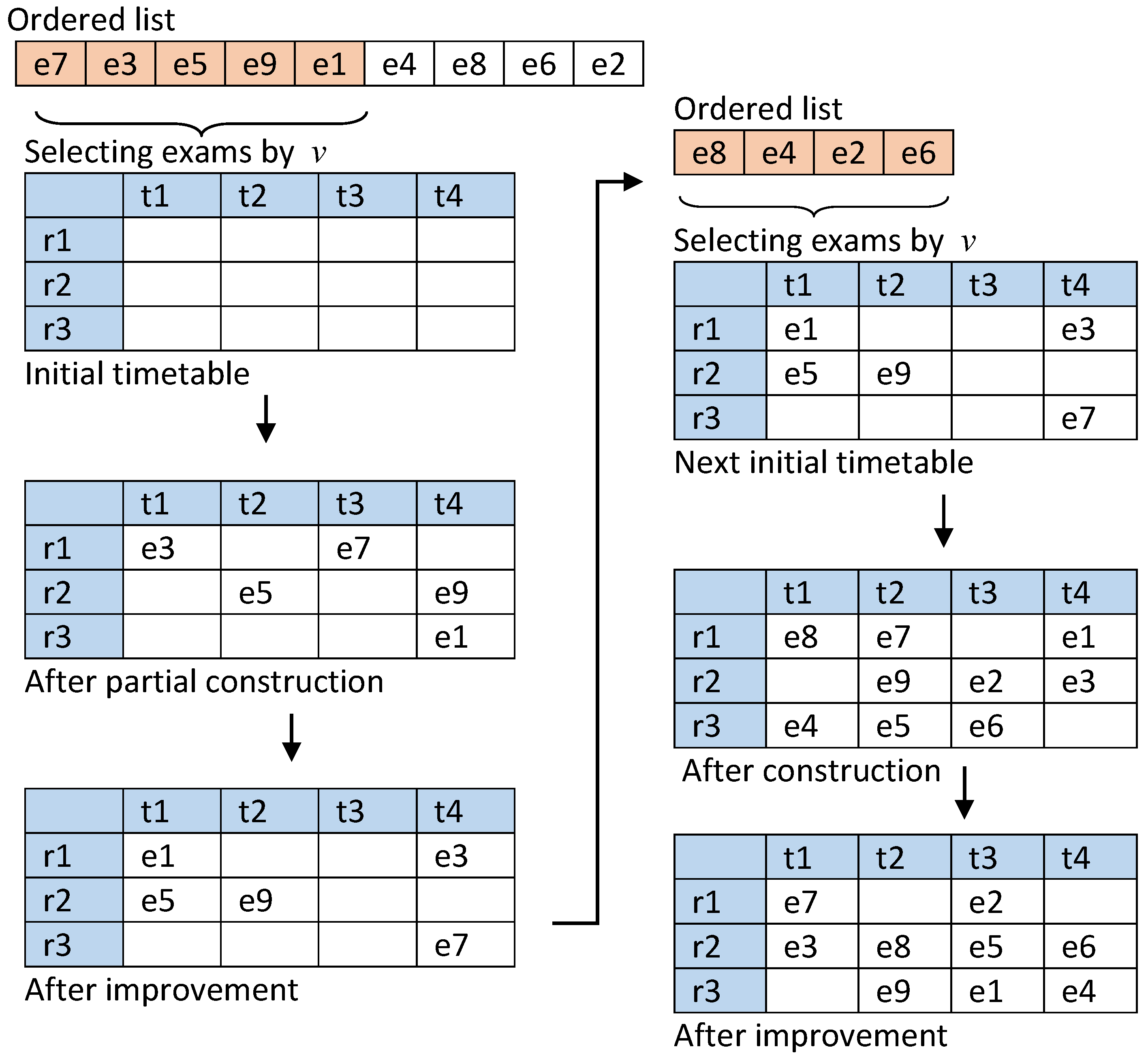
In this section, we describe the proposed PGH-mGD for the examination timetabling problem. The proposed approach partially schedules a group of exams that are selected based on a graph heuristic orderings and exam assignment value v. These partially scheduled exams are then improved using a modified GD algorithm. The procedure continues to schedule the next group of selected exams based on v and graph heuristic orderings. This above procedure repeats until the scheduling of all exams. The exam assignment value v plays an important role in the partial scheduling of the exams. This parameter can be defined in the following way: Supposing that N represents a list of exams, and v is an integer equal to or less than . Then v can be defined as the number of exams selected for scheduling (from the unscheduled list of exams). Here we have represented the v value as a percentage of the total exam N. For instance, if N is equal to 165, then 25% of v value would correspond to 41 (i.e., rounding of 41.25) exams being chosen for scheduling.
A simple example has been presented in Figure 1 to understand the overall PGH-mGD approach. Assuming that we have to schedule nine examinations and into four time slots and and three rooms and . Initially, the timetable is empty, and all nine examinations are ordered according to a graph heuristic ordering. Let us consider v is equal to 50%. Therefore, five exams (i.e., and ) will be selected for scheduling. These five exams are assigned into random time slots and rooms while ensuring feasibility is maintained, resulting in a partially constructed timetable. This timetable is then improved using a modified GD algorithm, aiming to reduce the penalty cost. After improving the timetable, the PGH-mGD will again select the next pool of exams (i.e., and ) from the ordered list that has been rearranged using a graph heuristic ordering. When four examinations are assigned properly, the timetable contains all nine examinations. The timetable is improved again, and finally, a complete timetable is returned.
4.2. PGH-mGD Algorithm
PGH-mGD deals with partial solutions followed by improvement until all exams have been scheduled. The PGH-mGD algorithm is shown in Algorithm 2. In addition to LD, LWD and LE orderings, here we use three hybrid graph heuristic orderings such as SD-LD, SD-LWD and SD-LE to measure the exam difficulty. For example, In SD-LD, exams are ordered according to SD followed with LD, and the exam at the top of the list is scheduled first. Initially, a graph heuristic ordering is selected from the heuristic list (line 1). The exam assignment value v is assigned, which indicates how many exams at a time will be scheduled (line 2). An iterative process starts with ordering the un-scheduled exams using a selected heuristic ordering (line 4). Next, a subset of exams is selected in sequence based on v from the ordered exams set (line 5). This subset of exams is called the current partial exams set. Fulfilling the required hard constraints, these partial exams are then scheduled into predefined time slots and rooms (for the ITC2007 exam dataset). During scheduling, if an exam fails to be assigned into a time slot (after several tries), an exam resolution manager is used, which attempts to handle these exams (line 6). The partial exam scheduling and exam resolution manager are described in Algorithms 3 and 4, respectively. When exams have been successfully scheduled, these exams are removed from the unscheduled exam set and inserted into the scheduled exam set (line 8). Next, the penalty cost is calculated based on the scheduled exams (line 9). In the next step, the modified GD algorithm (see Algorithm 5) is used to improve the quality of partially scheduled exams with the aim of satisfying the soft constraints (line 10). The above process repeats for the next batch of partial exams until all exams have been scheduled. Finally, the procedure checks whether the solution vector has satisfied all hard constraints (line 11), and no examinations are in the blacklist. The penalty value of the solution vector is then stored as the final solution (line 12).
| Algorithm 2. PGH-mGD approach. |
 |
| Algorithm 3. Scheduling partial exams. |
 |
4.3. Scheduling Procedure of Partial Exams
Algorithm 3 presents the partial exam scheduling procedure. In scheduling the exams, the selected exams are kept in a partial ordering list (line 1). An iterative procedure starts with selecting the first exam e in the list (line 3). A pseudo-random number is generated for time slot t and room r (for the ITC2007 exam dataset) for scheduling this exam (line 5). If the hard constraints are satisfied, the exam is removed from the partial ordering list and added to the partial scheduling list (line 8). Then, the next exam is selected for scheduling until all exams have been successfully scheduled. However, when it is not possible to schedule an exam after a few iterations (line 10), a mechanism called ExamResolutionManager (see Algorithm 4) is employed to assist the scheduling exam (line 11). If this mechanism can successfully schedule exam e, the exam is added to the partial scheduling list after being removed from the partial ordering list (lines 12–13). However, the exam e is moved to the blacklist when the mechanism fails to schedule the exam (lines 14–15). The above procedure repeats until the scheduling of all exams. The partial scheduling list is set as current partial scheduled examinations (line 16). Finally, if the blacklist contains unscheduled examinations, they are given high priority to be scheduled in the next attempt (line 17). That is, in the next partial ordering selection, blacklisted examinations are ordered (scheduled) first, followed by other examinations in the unscheduled list.
4.4. Exam Resolution Manager Procedure
Algorithm 4 illustrates the ExamResolutionManager procedure. As mentioned previously, when a particular exam cannot be scheduled (after several tries), it is considered as a complexExam (lines 1–2). From the current partial scheduling vector, the number of conflicting exams with complexExam in each time slot is calculated (lines 3–5). The time slots are then sorted in ascending order based on the number of conflicting exams (line 6). Next, the time slot that has less conflicted exams with the complexExam is chosen (line 8). The conflicting exams (with complexExam) are moved to a different time slot(s), ensuring feasibility (line 9). If they are moved successfully, the complexExam is assigned to the selected time slot and room of the timetable, the partial scheduled vector is updated, and the procedure is terminated indicating the success of scheduling the complexExam (lines 10–14). Otherwise, the next less-conflicted time slot is taken, and the same process is executed until all available time slots have been checked.
| Algorithm 4.ExamResolutionManager procedure. |
 |
4.5. Improvement Using Modified GD
Algorithm 5 shows the proposed modified GD algorithm used for improving the partially constructed solution. At the start, a partial solution vector s, generated from a graph heuristic ordering, is taken as an initial solution (Algorithm 3). The penalty value of this solution is calculated, which is also set as the initial boundary level B (lines 1–3). Then the number of iterations I, neighbourhood structure n, and desired value D are defined (lines 4–6). The decay rate is initialised dynamically as , and s is set as best solution (lines 7–8). Until the stopping condition is met, the following steps are executed. Neighbourhood structures are employed on the current solution s, and a set of new solutions is created. Among these solutions, one is considered as the candidate solution and its penalty cost is calculated (line 10). When this penalty cost is less than or equal to the current cost, or less than or equal to boundary level B, the candidate solution is set as a current solution (lines 11–12). Next, the current boundary level is updated as (line 13). The candidate solution is set as the best solution only if the penalty cost of this candidate solution is less than or equal to the cost of the best solution (lines 14–15). This algorithm encourages exploration by increasing the boundary level if the solution is not improved in M iterations (i.e., using the reheating mechanism [16,54]). Usually, a smaller value for M would encourage exploration, whereas a larger value would discourage exploration. Therefore, we have chosen M such a way that it can maintain the balance between exploration and exploitation. In this study, parameter M is set to 50 based on our preliminary experiment. The boundary level, B is then increased by adding a random number between 1 and 5 (line 17). Note that instead of standard formula (i.e., constant increment) to update the boundary level, the level is updated with a certain number (between 1 and 5 in this experiment) in order to allow some flexibility in accepting a worse solution. Abdullah et al. [17] also employed randomness in updating the boundary level and found efficiency for solving the timetabling problem. Finally, the best solution is returned as a partial best solution after the required number of iterations (line 18).
| Algorithm 5. Modified GD for improvement of partial scheduled exams. |
 |
5. TGH-mGD Algorithm
Algorithm 6 illustrates TGH-mGD approach that is implemented to compare with PGH-mGD. In TGH-mGD, the ordering uses six graph heuristic orderings which are LD, LWD, LE, SD-LD, SD-LWD and SD-LE. In each heuristic ordering, an initial feasible solution and its penalty cost are generated (lines 5–6). These steps are continued for 30 times for each of the heuristic orderings. Thirty iterations are chosen as we wish to generate a comparatively large pool of initial solutions for each of the instances. This will assist in selecting a good quality initial solution that will be employed in the improvement phase. After determining the best initial solution, an improvement phase is carried out using the same modified GD algorithm as described in Algorithm 5 (lines 7–8). Finally, the penalty cost is calculated. It is noted that during implementing modified GD in TGH-mGD, the only change is that instead of partial solution vector we use complete solution vector. ExamResolutionManager (see Algorithm 4) is also used when examinations have difficulty finding appropriate time slots and rooms.
| Algorithm 6. TGH-mGD approach. |
 |
6. Experimental Setup
Both PGH-mGD and TGH-mGD are validated with the Toronto and ITC2007 exam datasets. We examine the effect of exam assignment values v, graph heuristic orderings and execution time on solution quality. The experiment is repeated 30 times with different random seeds. The program is coded in Java (Java SE 7) and performed on a PC with following configurations: Intel Core i7 (3 GHz), 4 GB RAM and Windows 10 OS.
6.1. Toronto Dataset
For the Toronto benchmark dataset, twelve instances are tested. Four different v values are considered: 10%, 25%, 50% and 75%. Six different graph heuristic orderings including LD, LWD, LE, SD-LD, SD-LWD and SD-LE are employed in partial construction phases. Termination criterion for Toronto dataset is the time duration, and we investigate with three execution times such as 600 s, 1800 s and 3600 s. In the Toronto dataset, three neighbourhood structures are considered:
- : Move—an examination is randomly selected and moved to a random time slot.
- : Swap—Two examinations are randomly selected, and their time slots are swapped.
- : Swap time slot—Two time slots are randomly selected, and all examinations between the two time slots are swapped.
The above three neighbourhood structures are used during the improvement phase. However, we only accept neighbourhood moves that lead to an improvement.
6.2. ITC2007 Exam Dataset
We experiment with eight instances from the ITC2007 exam dataset. Six graph heuristic orderings LD, LWD, LE, SD-LD, SD-LWD and SD-LE are used to construct partial solutions. We use v = 5% and v = 10%. We experiment with two-time duration: 600 s and 3600 s. In the ITC2007 exam dataset, the following neighbourhood operations are employed:
- : An examination is randomly selected and is moved to a random time slot and room.
- : Two examinations are randomly selected, and their time slots and rooms are swapped.
- : After selecting an examination, it is moved to a different room within the same time slot.
- : Two examinations are selected randomly and moved to different time slots and rooms.
During the improvement phase, a neighbourhood (i.e., and ) is selected randomly and it is applied only if the solution is feasible; otherwise, a different neighbourhood structure will be selected.
It is noted that for both Toronto and ITC2007 exam datasets, the total execution time is divided among all partial improvement phases in such a way that the complete examination scheduling (i.e., last partial improvement phase) have sufficient time for improvement.
7. Experimental Result
In this section, we describe the results obtained from the experiment. The discussion starts with Toronto dataset followed by the ITC2007 dataset.
7.1. Experimental Results with Toronto Dataset
Table 4a–d present the performance of TGH-mGD and PGH-mGD when they are employed on the Toronto dataset using four different v values (i.e., 10%, 25%, 50%, and 75%) and with termination criteria: 600 s, 1800 s and 3600 s. We present the best and the average values for all problem instances. It is obvious from Table 4a–d that, with the same v value, the results with longer runs tend to outperform the results with a less amount of run (this is not surprising). Both TGH-mGD and PGH-mGD usually improve the solution quality. Using the same amount of run, the results with a lower v value are usually better than the results with a larger v value. Generally, we obtain better quality solutions when v = 10% with 3600 s compared to larger v value (i.e., 75%) with same amount of run (i.e., 3600 s). It is also noticed that in all the combinations of v and running time, the PGH-mGD outperforms TGH-mGD completely.
A comparative study of PGH-mGD with TGH-mGD is shown in Table 5. For all problem instances, PGH-mGD outperforms TGH-mGD. In car-s-91, maximum improvement of 17.92% is observed followed by car-f-92 and rye-s-93 which have around 16.50% and 14% improvement, respectively. For instances kfu-s-93, lse-f-91, tre-s-92 and ute-s-92, we obtain at least a 5% improvement, whereas for the other five instances, the improvement is below 4%. For eight instances, SD-LD produces the best results. This might be because the more conflicted exams are being prioritized. It is also observed that, on most occasions, a lower v tends to produce the best results. As can be seen, in the nine instances out of twelve, lower v (10%) produces the best results.
In a statistical analysis, we perform a t-test with a confidence level at 0.05. The null hypothesis () is that there is no difference between TGH-mGD and PGH-mGD, whereas the alternative hypothesis () states PGH-mGD performs better than TGH-mGD. Referring to Table 5, it is observed that the p-values of all instances are lower than the confidence level of 0.05, indicating that is rejected and is accepted. We therefore conclude that the performance of PGH-mGD is significantly better than TGH-mGD for the Toronto dataset.
7.2. Experimental Results with ITC2007 Exam Dataset
Table 6a,b present the penalty values for the ITC2007 exam dataset with and . The termination criteria is 600 s and 3600 s. Therefore, four different result sets are obtained. In all cases, we highlight the best and the average penalty costs for all the problem instances. Referring to Table 6a,b, when we increase the termination criterion from 600 s to 3600 s with the same v value, the penalty costs decrease for PGH-mGD (and TGH-mGD). However, when v value is increased from 5% to 10% (using the same time duration), the penalty values tend to be higher for PGH-mGD. We obtain the best results for most of the instances (6 out of 8 instances) with and time duration of 3600 s in PGH-mGD.
Comparison between TGH-mGD and PGH-mGD for ITC2007 exam dataset is shown in Table 7. For all of the eight instances, PGH-mGD produces better quality solutions compared to TGH-mGD. It is observed that a maximum improvement is obtained on Exam_2, with 59.14% improvement. Exam_3 and Exam_4 have around 50% improvement. Three exams including Exam_1, Exam_5 and Exam_7 have an average of around 40% improvement, whereas Exam_8 and Exam_6 obtain 30.45% and 13.61% improvement, respectively. We can see that PGH-mGD tends to improve the solution quality by employing lower v value, as six out of eight problem instances it produces the best results with . For all instances, hybrid graph heuristic orderings produce the best results as they can handle the complex exams well. We have carried out a t-test with a confidence level at 0.05. The null hypothesis () is that there is no difference between TGH-mGD and PGH-mGD, and the alternative hypothesis () is PGH-mGD performs better than TGH-mGD. The results indicate that p-values of all instances are smaller than the confidence level (0.05), indicating that is rejected, and is accepted. Therefore, the difference between these two approaches is significant for the ITC2007 exam dataset, with the performance of PGH-mGD being better than TGH-mGD.
7.3. Comparison with the State-of-the-Art Approaches
In this section, the proposed PGH-mGD has been compared with other approaches presented in the scientific literature for solving the Toronto and ITC2007 exam datasets. For each instance, we take the best results obtained from the PGH-mGD approach to compare with other reported results.
Ranking and average raking are computed in the following way. Let us consider total n approaches are compared for m given instances in terms of their best results. For a given instance, each approach of m is given ordinal value where and . This value indicates the ranking of the corresponding instance. Then each approach sums all its values for m instances and computes the average value. Finally, all of the approaches are ranked according to their average values.
7.3.1. Toronto Dataset
Table 8 presents the best results of the proposed approach with state-of-the-art methods on the Toronto dataset. We have ranked all the approaches according to the penalty costs (shown in brackets) of each instance. For each approach, the average rank of all Toronto instances is computed.
It is observed from Table 8 that we have been able to produce solutions for all of the twelve instances of the Toronto dataset. Our approach outperforms Sabar et al. [9] and Alinia Ahandani et al. [27] in all problem instances. Apart from instance rye-s-93, for all other instances, our approach achieves better results than the approaches proposed by Carter et al. [5], Abdul Rahman et al. [41], Pillay and Banzhaf [8], Qu et al. [55] and Nelishia Pillay and Özcan [35]. Moreover, we have obtained better results than the results reported by Turabieh and Abdullah [56] for all instances except for kfu-s-93, lse-f-91 and rye-s-93. For six instances (car-s-91, car-f-92, ear-f-83, rye-s-93, tre-s-92, uta-s-92), we have produced better results than Burke et al. [57]. While comparing among all approaches, our approach has produced the best results for five instances car-s-91, car-f-92, ear-f-83, tre-s-92 and uta-s-92, and the second best results for instances hec-s-92, kfu-s-93, sta-f-83, ute-s-92 and yor-f-83. Besides, for one instance lse-f-91 we have obtained the third best result. Finally, when we compare the average rank of the approaches, our approach is ranked first in solving all problem instances of the Toronto dataset.
7.3.2. ITC2007 Exam Dataset
Table 9 highlights the comparison of our proposed approach with some results from the scientific literature on ITC2007 exam dataset. For each problem instance, we rank all of the approaches based on their penalty values. The rank value is shown next to the penalty value of each problem instance. We also compute the average rank for each approach for solving the overall ITC2007 exam dataset.
It is observed from Table 9 that Müller [14] produces the best results for five out of eight instances, and its average rank is the highest. Besides, Alzaqebah and Abdullah [58] is in second place in terms of average rank. Our approach is ranked in the third position among the ten approaches. We were able to produce the best results for Exam_6, the second best result for Exam_2, and the third best result for both Exam_4 and Exam_8. Overall, our approach shows comparable results with other approaches in solving all of the instances of ITC2007 exam dataset.
8. Discussion and Analysis
It is clear from the above experimental results that the PGH-mGD approach performs better than the TGH-mGD approach for solving both Toronto and ITC2007 exam datasets. It is also observed that lower v, the longer time duration and hybrid graph heuristic orderings can reduce the penalty costs (i.e., produce quality solutions) in the PGH-mGD approach. Our best results are comparable with the reported results from the scientific literature (see Table 8 and Table 9), with several cases producing the best results. The PGH-mGD approach can produce feasible solutions for all datasets because the ExamResolutionManager procedure helps to handle any deadlock faced during the scheduling process. As ITC2007 exam dataset is a heavily constraint problem compared to Toronto dataset, the ExamResolutionManager procedure is used more often in the ITC2007 exam dataset than in the Toronto dataset. One limitation of the partial examination approach is that in the case of some examinations with high conflict densities and complex hard constraints, it is occasionally stuck in obtaining feasible solutions, thus increasing the computational time.
In TGH-mGD, a good initial solution is first chosen from the construction phase, and then it is improved so that a good final solution is obtained. According to Kahar and Kendall [16], it is observed that in a sequential (i.e., traditional) approach, good initial solution(s) tend to produce good improved solution(s). However, with the partial examination assignment approach, we can improve the partial solution many times, especially with small v, and this improvement activity encourages the improvement phase to produce a good quality solution. Additionally, modified GD promotes exploration (with the reheating mechanism), allowing the search to escape from local optima. Hence the partial examination assignment approach (i.e., PGH-mGD) is able to produce quality solutions (for all instances) compared to the traditional approach (i.e., TGH-mGD).
9. Conclusions and Future Work
In this paper, a partial exam assignment strategy has been proposed for addressing the examination timetabling problem. In this approach, partially selected exams that are obtained based on a parameter named exam assignment value v are constructed using graph heuristic orderings, and then solution quality is improved using a modified GD algorithm until all exams have been scheduled. Both TGH-mGD and PGH-mGD are tested on two different benchmark datasets—Toronto and ITC2007 exam track, with each benchmark having its own distinctive features. Experimental results and statistical analysis indicate that PGH-mGD produces better results compared to the TGH-mGD algorithm for all instances of the datasets. To study the effectiveness of the proposed approach, we experiment with different v values, termination criteria (time duration) and graph heuristic orderings. It is observed that, with smaller v and the longer time duration, PGH-mGD approach tends to produce quality solutions. In comparison with state-of-the-art methods, our approach has produced the five best results for the Toronto dataset, with promising results obtained for other seven instances of the dataset. Although we have produced one best result for the ITC2007 exam dataset, our obtained results of other instances are competitive with the reported results from the scientific literature. For future work, the following suggestions might be worthy of investigation.
- The partial construction phase could be extended and improved by introducing adapting ordering strategies or fuzzy logic that may select the appropriate heuristics (i.e., LD, LE, LWD) for exam ordering.
- The partial improvement phase can also be improved by incorporating other meta-heuristic approaches, such as SA, tabu search and genetic algorithms, or hybridising of meta-heuristics.
- This paper has studied the impact of different exam assignment value v on the penalty cost. However, it would be worthwhile to study the effect of dynamic or adaptive exam assignment value on the penalty cost.
Author Contributions
Conceptualization, A.K.M. and M.N.M.K.; methodology, A.K.M.; software, A.K.M.; validation, A.K.M., M.N.M.K. and G.K.; formal analysis, A.K.M.; investigation, M.N.M.K. and G.K.; writing—original draft preparation, A.K.M.; writing—review and editing, M.N.M.K. and G.K. All authors have read and agreed to the published version of the manuscript.
Funding
This research received no external funding.
Acknowledgments
This work was supported by University Malaysia Pahang (UMP), Malaysia.
Conflicts of Interest
The authors declare no conflict of interest.
Abbreviations
The following abbreviations are used in this manuscript:
| PGH-mGD | Partial graph heuristic orderings with a modified great deluge |
| TGH-mGD | Traditional graph heuristic orderings with a modified great deluge |
| ITC2007 | 2nd International Timetable Competition |
| LD | Largest degree |
| LWD | Largest weighted degree |
| LE | Largest enrolment |
| SD | Saturation degree |
| GD | Great deluge |
| SD-LD | Saturation degree - Largest degree |
| SD-LWD | Saturation degree -Largest weighted Degree |
| SD-LE | Saturation degree- Largest enrolment |
References
- Wren, A. Scheduling, timetabling and rostering—A special relationship. In Practice and Theory of Automated Timetabling; Springer: Berlin/Heidelberg, Germany, 1996; pp. 46–75. [Google Scholar]
- Johnson, D. Timetabling university examinations. J. Oper. Res. Soc. 1990, 41, 39–47. [Google Scholar] [CrossRef]
- Burke, E.K.; Newall, J.P. Solving examination timetabling problems through adaption of heuristic orderings. Ann. Oper. Res. 2004, 129, 107–134. [Google Scholar] [CrossRef]
- Burke, E.K.; Petrovic, S.; Qu, R. Case-based heuristic selection for timetabling problems. J. Sched. 2006, 9, 115–132. [Google Scholar] [CrossRef] [Green Version]
- Carter, M.W.; Laporte, G.; Lee, S.Y. Examination timetabling: Algorithmic strategies and applications. J. Oper. Res. Soc. 1996, 47, 373–383. [Google Scholar] [CrossRef]
- Kahar, M.N.M.; Kendall, G. The examination timetabling problem at Universiti Malaysia Pahang: Comparison of a constructive heuristic with an existing software solution. Eur. J. Oper. Res. 2010, 207, 557–565. [Google Scholar] [CrossRef]
- Asmuni, H.; Burke, E.K.; Garibaldi, J.M.; McCollum, B.; Parkes, A.J. An investigation of fuzzy multiple heuristic orderings in the construction of university examination timetables. Comput. Oper. Res. 2009, 36, 981–1001. [Google Scholar] [CrossRef] [Green Version]
- Pillay, N.; Banzhaf, W. A study of heuristic combinations for hyper-heuristic systems for the uncapacitated examination timetabling problem. Eur. J. Oper. Res. 2009, 197, 482–491. [Google Scholar] [CrossRef]
- Sabar, N.R.; Ayob, M.; Qu, R.; Kendall, G. A graph coloring constructive hyper-heuristic for examination timetabling problems. Appl. Intell. 2012, 37, 1–11. [Google Scholar] [CrossRef]
- Dueck, G. New optimization heuristics: The great deluge algorithm and the record-to-record travel. J. Comput. Phys. 1993, 104, 86–92. [Google Scholar] [CrossRef]
- Burke, E.K.; Newall, J.P. Enhancing timetable solutions with local search methods. In Practice and Theory of Automated Timetabling IV; Springer: Berlin/Heidelberg, Germany, 2003; pp. 195–206. [Google Scholar]
- Burke, E.K.; Bykov, Y. Solving exam timetabling problems with the flex-deluge algorithm. In Proceedings of the 6th International Conference on the Practice and Theory of Automated Timetabling (PTATA 2006), Brno, Czech Republic, 30 August–1 September 2006; pp. 370–372. [Google Scholar]
- Landa-Silva, D.; Obit, J.H. Great deluge with non-linear decay rate for solving course timetabling problems. In Proceedings of the 4th International IEEE Conference on Intelligent Systems, Varna, Bulgaria, 6–8 September 2008; Volume 1, pp. 11–18. [Google Scholar] [CrossRef]
- Müller, T. ITC2007 solver description: A hybrid approach. Ann. Oper. Res. 2009, 172, 429–446. [Google Scholar] [CrossRef] [Green Version]
- McCollum, B.; McMullan, P.; Parkes, A.J.; Burke, E.K.; Abdullah, S. An extended great deluge approach to the examination timetabling problem. In Proceedings of the 4th multidisciplinary international scheduling: Theory and applications 2009 (MISTA 2009), Dublin, Ireland, 10–12 August 2009; pp. 424–434. [Google Scholar]
- Kahar, M.N.M.; Kendall, G. A great deluge algorithm for a real-world examination timetabling problem. J. Oper. Res. Soc. 2013, 66, 16–133. [Google Scholar] [CrossRef]
- Abdullah, S.; Shaker, K.; McCollum, B.; McMullan, P. Construction of course timetables based on great deluge and tabu search. In Proceedings of the MIC 2009: VIII Metaheuristic International Conference, Hamburg, Germany, 13–16 July 2009; pp. 13–16. [Google Scholar]
- Turabieh, H.; Abdullah, S. An integrated hybrid approach to the examination timetabling problem. Omega Int. J. Manag. Sci. 2011, 39, 598–607. [Google Scholar] [CrossRef]
- Fong, C.W.; Asmuni, H.; McCollum, B.; McMullan, P.; Omatu, S. A new hybrid imperialist swarm-based optimization algorithm for university timetabling problems. Inf. Sci. 2014, 283, 1–21. [Google Scholar] [CrossRef]
- Abuhamdah, A. Modified Great Deluge for Medical Clustering Problems. Int. J. Emerg. Sci. 2012, 2, 345–360. [Google Scholar]
- Kifah, S.; Abdullah, S. An adaptive non-linear great deluge algorithm for the patient-admission problem. Inf. Sci. 2015, 295, 573–585. [Google Scholar] [CrossRef]
- Jaddi, N.S.; Abdullah, S. Nonlinear great deluge algorithm for rough set attribute reduction. J. Inf. Sci. Eng. 2013, 29, 49–62. [Google Scholar]
- Burke, E.K.; Bykov, Y. The Late Acceptance Hill-Climbing Heuristic; Technical Report CSM-192, Computing Science and Mathematics; University of Stirling: Stirling, UK, 2012. [Google Scholar]
- Burke, E.K.; Bykov, Y. An Adaptive Flex-Deluge Approach to University Exam Timetabling. INFORMS J. Comput. 2016, 28, 781–794. [Google Scholar] [CrossRef]
- Battistutta, M.; Schaerf, A.; Urli, T. Feature-based tuning of single-stage simulated annealing for examination timetabling. Ann. Oper. Res. 2017, 252, 239–254. [Google Scholar] [CrossRef]
- June, T.L.; Obit, J.H.; Leau, Y.B.; Bolongkikit, J. Implementation of Constraint Programming and Simulated Annealing for Examination Timetabling Problem. In Computational Science and Technology; Springer: Berlin/Heidelberg, Germany, 2019; pp. 175–184. [Google Scholar]
- Alinia Ahandani, M.; Vakil Baghmisheh, M.T.; Badamchi Zadeh, M.A.; Ghaemi, S. Hybrid particle swarm optimization transplanted into a hyper-heuristic structure for solving examination timetabling problem. Swarm Evol. Comput. 2012, 7, 21–34. [Google Scholar] [CrossRef]
- Abayomi-Alli, O.; Abayomi-Alli, A.; Misra, S.; Damasevicius, R.; Maskeliunas, R. Automatic examination timetable scheduling using particle swarm optimization and local search algorithm. In Data, Engineering and Applications; Springer: Berlin/Heidelberg, Germany, 2019; pp. 119–130. [Google Scholar]
- Bolaji, A.L.; Khader, A.T.; Al-Betar, M.A.; Awadallah, M.A. A hybrid nature-inspired artificial bee colony algorithm for uncapacitated examination timetabling problems. J. Intell. Syst. 2015, 24, 37–54. [Google Scholar] [CrossRef]
- Tilahun, S.L. Prey-predator algorithm for discrete problems: A case for examination timetabling problem. Turk. J. Electr. Eng. Comput. Sci. 2019, 27, 950–960. [Google Scholar] [CrossRef]
- Lei, Y.; Gong, M.; Jiao, L.; Shi, J.; Zhou, Y. An adaptive coevolutionary memetic algorithm for examination timetabling problems. Int. J. Bio-Inspired Comput. 2017, 10, 248–257. [Google Scholar] [CrossRef]
- Leite, N.; Fernandes, C.M.; Melicio, F.; Rosa, A.C. A cellular memetic algorithm for the examination timetabling problem. Comput. Oper. Res. 2018, 94, 118–138. [Google Scholar] [CrossRef]
- Demeester, P.; Bilgin, B.; De Causmaecker, P.; Vanden Berghe, G. A hyperheuristic approach to examination timetabling problems: Benchmarks and a new problem from practice. J. Sched. 2012, 15, 83–103. [Google Scholar] [CrossRef]
- Anwar, K.; Khader, A.T.; Al-Betar, M.A.; Awadallah, M.A. Harmony Search-based Hyper-heuristic for examination timetabling. In Proceedings of the 9th IEEE International Colloquium on Signal Processing and its Applications (CSPA), Kuala Lumpur, Malaysia, 8–10 March 2013; pp. 176–181. [Google Scholar] [CrossRef]
- Pillay, N.; Özcan, E. Automated generation of constructive ordering heuristics for educational timetabling. Ann. Oper. Res. 2019, 275, 181–208. [Google Scholar] [CrossRef] [Green Version]
- Gogos, C.; Alefragis, P.; Housos, E. An improved multi-staged algorithmic process for the solution of the examination timetabling problem. Ann. Oper. Res. 2012, 194, 203–221. [Google Scholar] [CrossRef]
- Burke, E.K.; Pham, N.; Qu, R.; Yellen, J. Linear combinations of heuristics for examination timetabling. Ann. Oper. Res. 2012, 194, 89–109. [Google Scholar] [CrossRef]
- Ei Shwe, S. Reinforcement learning with EGD based hyper heuristic system for exam timetabling problem. In Proceedings of the 2011 IEEE International Conference on Cloud Computing and Intelligence Systems (CCIS), Beijing, China, 15–17 September 2011; pp. 462–466. [Google Scholar] [CrossRef]
- Sabar, N.R.; Ayob, M.; Kendall, G.; Qu, R. Automatic Design of a Hyper-Heuristic Framework With Gene Expression Programming for Combinatorial Optimization Problems. IEEE Trans. Evol. Comput. 2015, 19, 309–325. [Google Scholar] [CrossRef] [Green Version]
- Qu, R.; Burke, E.; McCollum, B.; Merlot, L.; Lee, S. A survey of search methodologies and automated system development for examination timetabling. J. Sched. 2009, 12, 55–89. [Google Scholar] [CrossRef]
- Abdul Rahman, S.; Bargiela, A.; Burke, E.K.; Özcan, E.; McCollum, B.; McMullan, P. Adaptive linear combination of heuristic orderings in constructing examination timetables. Eur. J. Oper. Res. 2014, 232, 287–297. [Google Scholar] [CrossRef] [Green Version]
- Soghier, A.; Qu, R. Adaptive selection of heuristics for assigning time slots and rooms in exam timetables. Appl. Intell. 2013, 39, 438–450. [Google Scholar] [CrossRef]
- Eng, K.; Muhammed, A.; Mohamed, M.A.; Hasan, S. A hybrid heuristic of Variable Neighbourhood Descent and Great Deluge algorithm for efficient task scheduling in Grid computing. Eur. J. Oper. Res. 2020, 284, 75–86. [Google Scholar] [CrossRef]
- Obit, J.H.; Landa-Silva, D. Computational study of non-linear great deluge for university course timetabling. In Intelligent Systems: From Theory to Practice; Springer: Berlin/Heidelberg, Germany, 2010; pp. 309–328. [Google Scholar]
- Bagayoko, M.; Dao, T.M.; Ateme-Nguema, B.H. Optimization of forest vehicle routing using the metaheuristics: Reactive tabu search and extended great deluge. In Proceedings of the 2013 International Conference on Industrial Engineering and Systems Management (IESM), Rabat, Morocco, 28–30 October 2013; pp. 1–7. [Google Scholar]
- Guha, R.; Ghosh, M.; Kapri, S.; Shaw, S.; Mutsuddi, S.; Bhateja, V.; Sarkar, R. Deluge based Genetic Algorithm for feature selection. Evolut. Intell. 2019. [Google Scholar] [CrossRef]
- Mafarja, M.; Abdullah, S. Fuzzy modified great deluge algorithm for attribute reduction. In Recent Advances on Soft Computing and Data Mining; Springer: Berlin/Heidelberg, Germany, 2014; pp. 195–203. [Google Scholar]
- Nahas, N.; Nourelfath, M. Iterated great deluge for the dynamic facility layout problem. In Metaheuristics for Production Systems; Springer: Berlin/Heidelberg, Germany, 2016; pp. 57–92. [Google Scholar]
- Benchmark Data Sets in Exam Timetabling. Available online: http://www.asap.cs.nott.ac.uk/resources/data.shtml (accessed on 30 November 2019).
- Examination Timetabling Track. Available online: http://www.cs.qub.ac.uk/itc2007/examtrack/ (accessed on 30 November 2019).
- McCollum, B.; McMullan, P.; Parkes, A.J.; Burke, E.K.; Qu, R. A new model for automated examination timetabling. Ann. Oper. Res. 2012, 194, 291–315. [Google Scholar] [CrossRef]
- McCollum, B.; McMullan, P.; Burke, E.K.; Parkes, A.J.; Qu, R. The Second International Timetabling Competition: Examination Timetabling Track; Technical Report QUB/IEEE/Tech/ITC2007/Exam/v4. 0/17; Queen’s University: Belfast, UK, 2007. [Google Scholar]
- Burke, E.K.; Kingston, J.; De Werra, D. Applications to Timetabling. In Handbook of Graph Theory; Rosen, K.H., Ed.; CRC Press: Boca Raton, FL, USA, 2004; pp. 445–474. [Google Scholar]
- Abdullah, S.; Turabieh, H.; McCollum, B.; McMullan, P. A hybrid metaheuristic approach to the university course timetabling problem. J. Heuristics 2012, 18, 1–23. [Google Scholar] [CrossRef] [Green Version]
- Qu, R.; Pham, N.; Bai, R.B.; Kendall, G. Hybridising heuristics within an estimation distribution algorithm for examination timetabling. Appl. Intell. 2015, 42, 679–693. [Google Scholar] [CrossRef] [Green Version]
- Turabieh, H.; Abdullah, S. A Hybrid Fish Swarm Optimisation Algorithm for Solving Examination Timetabling Problems. In Learning and Intelligent Optimization; Lecture Notes in Computer Science; Book Section 42; Coello, C.C., Ed.; Springer: Berlin/Heidelberg, Germany, 2011; Volume 6683, pp. 539–551. [Google Scholar] [CrossRef]
- Burke, E.K.; Eckersley, A.J.; McCollum, B.; Petrovic, S.; Qu, R. Hybrid variable neighbourhood approaches to university exam timetabling. Eur. J. Oper. Res. 2010, 206, 46–53. [Google Scholar] [CrossRef] [Green Version]
- Alzaqebah, M.; Abdullah, S. Hybrid bee colony optimization for examination timetabling problems. Comput. Oper. Res. 2015, 54, 142–154. [Google Scholar] [CrossRef]
- Gogos, C.; Alefragis, P.; Housos, P. Amulti-staged algorithmic process for the solution of the examination timetabling problem. In Proceedings of the 7th International Conference on the Practice and Theory of Automated Timetabling (PATAT 2008), Montreal, QC, Canada, 18–22 August 2008; pp. 19–22. [Google Scholar]
- Atsuta, M.; Nonobe, K.; Ibaraki, T. ITC-2007 Track2: An Approach Using General CSP Solver. In Proceedings of the Practice and Theory of Automated Timetabling (PATAT 2008), Montreal, QC, Canada, 19–22 August 2008. [Google Scholar]
- De Smet, G. ITC2007—Examination track. In Proceedings of the 7th International Conference on the Practice and Theory of Automated Timetabling (PATAT 2008), Montreal, QC, Canada, 18–22 August 2008. [Google Scholar]
- Pillay, N.; Banzhaf, W. A Developmental Approach to the Uncapacitated Examination Timetabling Problem. In Parallel Problem Solving from Nature—PPSN X. PPSN 2008; Rudolph, G., Jansen, T., Beume, N., Lucas, S., Poloni, C., Eds.; Lecture Notes in Computer Science; Springer: Berlin/Heidelberg, Germany, 2008; Volume 5199. [Google Scholar]
- Hamilton-Bryce, R.; McMullan, P.; McCollum, B. Directed selection using reinforcement learning for the examination timetabling problem. In Proceedings of the PATAT’14 Proceedings of the 10th International Conference on the Practice and Theory of Automated Timetabling, York, UK, 26–29 August 2014. [Google Scholar]
Figure 1.
An Illustration of PGH-mGD for examination timetabling procedure.


Table 1.
Toronto Benchmark dataset.
| Instances | No. of Time Slots | No. of Exams | No. of Students | Conflict Density |
|---|---|---|---|---|
| car-s-91 | 35 | 682 | 16,925 | 0.13 |
| car-f-92 | 32 | 543 | 18,419 | 0.14 |
| ear-f-83 | 24 | 190 | 1125 | 0.27 |
| hec-s-92 | 18 | 81 | 2823 | 0.42 |
| kfu-s-93 | 20 | 461 | 5349 | 0.06 |
| lse-f-91 | 18 | 381 | 2726 | 0.06 |
| pur-s-93 | 42 | 2419 | 30,029 | 0.03 |
| rye-s-93 | 23 | 486 | 11,483 | 0.07 |
| sta-f-83 | 13 | 139 | 611 | 0.14 |
| tre-s-92 | 23 | 261 | 4360 | 0.18 |
| uta-s-92 | 35 | 622 | 21,267 | 0.13 |
| ute-s-92 | 10 | 184 | 2750 | 0.08 |
| yor-f-83 | 21 | 181 | 941 | 0.29 |
Table 2.
ITC2007 Exam Dataset.
| Instances | Number of Students | Number of Exams | Number of Time slots | Number of Rooms | Period Hard Constraint | Room Hard Constraint | Conflict Density |
|---|---|---|---|---|---|---|---|
| Exam_1 | 7833 | 607 | 54 | 7 | 12 | 0 | 5.05% |
| Exam_2 | 12,484 | 870 | 40 | 49 | 12 | 2 | 1.17% |
| Exam_3 | 16,365 | 934 | 36 | 48 | 170 | 15 | 2.62% |
| Exam_4 | 4421 | 273 | 21 | 1 | 40 | 0 | 15.0% |
| Exam_5 | 8719 | 1018 | 42 | 3 | 27 | 0 | 0.87% |
| Exam_6 | 7909 | 242 | 16 | 8 | 23 | 0 | 6.16% |
| Exam_7 | 13,795 | 1096 | 80 | 15 | 28 | 0 | 1.93% |
| Exam_8 | 7718 | 598 | 80 | 8 | 20 | 1 | 4.55% |
Table 3.
Weights of the ITC2007 exam dataset.
| Instances | Weight for Two in a Day | Weight for Two in a Row | Weight for Period Spread | Weight for No Mixed Duration | Weight for the Front Load Penalty | Weight for period Penalty | Weight for Room Penalty |
|---|---|---|---|---|---|---|---|
| Exam_1 | 5 | 7 | 5 | 10 | 100 | 30 | 5 |
| Exam_2 | 5 | 15 | 1 | 25 | 250 | 30 | 5 |
| Exam_3 | 10 | 15 | 4 | 20 | 200 | 20 | 10 |
| Exam_4 | 5 | 9 | 2 | 10 | 50 | 10 | 5 |
| Exam_5 | 15 | 40 | 5 | 0 | 250 | 30 | 10 |
| Exam_6 | 5 | 20 | 20 | 25 | 25 | 30 | 15 |
| Exam_7 | 5 | 25 | 10 | 15 | 250 | 30 | 10 |
| Exam_8 | 0 | 150 | 15 | 25 | 250 | 30 | 5 |
Table 4.
Penalty values of Toronto dataset for different termination criteria
(a) v = 10% for PGH-mGD
| Instances | 600 s | 1800 s | 3600 s | |||||||||
|---|---|---|---|---|---|---|---|---|---|---|---|---|
| TGH-mGD | PGH-mGD | TGH-mGD | PGH-mGD | TGH-mGD | PGH-mGD | |||||||
| Best | Avg | Best | Avg | Best | Avg | Best | Avg | Best | Avg | Best | Avg | |
| car-s-91 | 5.98 | 6.19 | 5.69 | 5.83 | 5.78 | 5.99 | 5.60 | 5.69 | 5.58 | 5.70 | 4.58 | 4.72 |
| car-f-92 | 4.95 | 5.11 | 4.66 | 4.78 | 4.80 | 4.95 | 4.57 | 4.69 | 4.58 | 4.66 | 3.82 | 3.93 |
| ear-f-83 | 38.67 | 40.46 | 37.00 | 38.69 | 37.23 | 39.24 | 36.35 | 37.33 | 33.68 | 34.76 | 33.23 | 34.49 |
| hec-s-92 | 11.92 | 12.19 | 11.25 | 11.91 | 11.44 | 11.92 | 11.18 | 11.75 | 10.53 | 11.02 | 10.32 | 11.09 |
| kfu-s-93 | 15.65 | 16.80 | 14.61 | 15.43 | 15.37 | 16.09 | 14.44 | 14.91 | 14.79 | 15.10 | 13.34 | 13.97 |
| lse-f-91 | 12.75 | 13.61 | 11.78 | 12.34 | 12.40 | 12.99 | 11.05 | 11.47 | 10.85 | 11.12 | 10.24 | 10.62 |
| rye-s-93 | 11.90 | 12.24 | 11.44 | 11.89 | 11.71 | 11.88 | 11.25 | 11.71 | 11.39 | 11.54 | 9.79 | 10.29 |
| sta-f-83 | 158.21 | 158.48 | 157.66 | 158.28 | 157.86 | 158.14 | 157.50 | 158.19 | 157.39 | 157.72 | 157.14 | 157.64 |
| tre-s-92 | 9.42 | 9.80 | 8.58 | 8.88 | 9.21 | 9.49 | 8.20 | 8.44 | 8.24 | 8.50 | 7.74 | 8.03 |
| uta-s-92 | 4.12 | 4.17 | 3.70 | 3.82 | 3.93 | 4.04 | 3.61 | 3.68 | 3.22 | 3.29 | 3.13 | 3.22 |
| ute-s-92 | 28.49 | 29.47 | 27.38 | 28.61 | 28.04 | 28.82 | 27.08 | 27.83 | 26.96 | 27.79 | 25.28 | 26.04 |
| yor-f-83 | 40.44 | 41.35 | 39.00 | 40.43 | 39.52 | 40.22 | 38.34 | 39.39 | 35.51 | 36.71 | 35.68 | 36.79 |
(b) v = 25% for PGH-mGD
| Instances | 600 s | 1800 s | 3600 s | |||||||||
|---|---|---|---|---|---|---|---|---|---|---|---|---|
| TGH-mGD | PGH-mGD | TGH-mGD | PGH-mGD | TGH-mGD | PGH-mGD | |||||||
| Best | Avg | Best | Avg | Best | Avg | Best | Avg | Best | Avg | Best | Avg | |
| car-s-91 | 5.98 | 6.19 | 5.63 | 5.82 | 5.78 | 5.99 | 5.57 | 5.67 | 5.58 | 5.70 | 4.60 | 4.68 |
| car-f-92 | 4.95 | 5.11 | 4.68 | 4.85 | 4.80 | 4.95 | 4.63 | 4.71 | 4.58 | 4.66 | 3.89 | 4.04 |
| ear-f-83 | 38.67 | 40.46 | 36.82 | 38.89 | 37.23 | 39.24 | 35.93 | 37.83 | 33.68 | 34.76 | 33.30 | 34.43 |
| hec-s-92 | 11.92 | 12.19 | 11.31 | 12.05 | 11.44 | 11.92 | 11.23 | 11.78 | 10.53 | 11.02 | 10.49 | 11.09 |
| kfu-s-93 | 15.65 | 16.80 | 14.71 | 15.57 | 15.37 | 16.09 | 14.60 | 15.27 | 14.79 | 15.10 | 13.55 | 14.34 |
| lse-f-91 | 12.75 | 13.61 | 12.06 | 12.67 | 12.40 | 12.99 | 11.46 | 12.10 | 10.85 | 11.12 | 10.25 | 10.76 |
| rye-s-93 | 11.90 | 12.24 | 11.40 | 11.86 | 11.71 | 11.88 | 11.38 | 11.71 | 11.39 | 11.54 | 10.68 | 11.20 |
| sta-f-83 | 158.21 | 158.48 | 157.71 | 158.34 | 157.86 | 158.14 | 157.70 | 158.12 | 157.39 | 157.72 | 157.03 | 157.41 |
| tre-s-92 | 9.42 | 9.80 | 8.79 | 9.06 | 9.21 | 9.49 | 8.56 | 8.85 | 8.24 | 8.50 | 7.94 | 8.15 |
| uta-s-92 | 4.12 | 4.17 | 3.77 | 3.88 | 3.93 | 4.04 | 3.61 | 3.74 | 3.22 | 3.29 | 3.17 | 3.26 |
| ute-s-92 | 28.49 | 29.47 | 27.97 | 28.85 | 28.04 | 28.82 | 27.56 | 28.53 | 26.96 | 27.79 | 25.47 | 25.95 |
| yor-f-83 | 40.44 | 41.35 | 39.18 | 40.78 | 39.52 | 40.22 | 39.11 | 40.06 | 35.51 | 36.71 | 35.68 | 36.91 |
(c) v = 50% for PGH-mGD
| Instances | 600 s | 1800 s | 3600 s | |||||||||
|---|---|---|---|---|---|---|---|---|---|---|---|---|
| TGH-mGD | PGH-mGD | TGH-mGD | PGH-mGD | TGH-mGD | PGH-mGD | |||||||
| Best | Avg | Best | Avg | Best | Avg | Best | Avg | Best | Avg | Best | Avg | |
| car-s-91 | 5.98 | 6.19 | 5.82 | 6.05 | 5.78 | 5.99 | 4.63 | 4.80 | 5.58 | 5.70 | 4.09 | 4.41 |
| car-f-92 | 4.95 | 5.11 | 4.81 | 5.00 | 4.80 | 4.95 | 5.56 | 5.72 | 4.58 | 4.66 | 4.63 | 4.74 |
| ear-f-83 | 38.67 | 40.46 | 36.91 | 39.11 | 37.23 | 39.24 | 36.28 | 38.13 | 33.68 | 34.76 | 33.43 | 34.68 |
| hec-s-92 | 11.92 | 12.19 | 11.70 | 12.13 | 11.44 | 11.92 | 11.41 | 11.92 | 10.53 | 11.02 | 10.59 | 11.17 |
| kfu-s-93 | 15.65 | 16.80 | 15.12 | 15.86 | 15.37 | 16.09 | 14.78 | 15.38 | 14.79 | 15.10 | 13.51 | 14.46 |
| lse-f-91 | 12.75 | 13.61 | 12.44 | 13.10 | 12.40 | 12.99 | 11.75 | 12.45 | 10.85 | 11.12 | 10.50 | 10.99 |
| rye-s-93 | 11.90 | 12.24 | 11.62 | 12.08 | 11.71 | 11.88 | 11.47 | 11.86 | 11.39 | 11.54 | 11.24 | 11.55 |
| sta-f-83 | 158.21 | 158.48 | 157.86 | 158.40 | 157.86 | 158.14 | 157.43 | 158.05 | 157.39 | 157.72 | 157.15 | 157.54 |
| tre-s-92 | 9.42 | 9.80 | 9.00 | 9.20 | 9.21 | 9.49 | 8.77 | 8.99 | 8.24 | 8.50 | 8.03 | 8.22 |
| uta-s-92 | 4.12 | 4.17 | 3.85 | 4.02 | 3.93 | 4.04 | 3.77 | 3.88 | 3.22 | 3.29 | 3.26 | 3.36 |
| ute-s-92 | 28.49 | 29.47 | 28.26 | 29.00 | 28.04 | 28.82 | 27.68 | 28.40 | 26.96 | 27.79 | 25.52 | 26.57 |
| yor-f-83 | 40.44 | 41.35 | 39.34 | 41.00 | 39.52 | 40.22 | 38.99 | 40.19 | 35.51 | 36.71 | 35.46 | 36.75 |
(d) v = 75% for PGH-mGD
| Instances | 600 s | 1800 s | 3600 s | |||||||||
|---|---|---|---|---|---|---|---|---|---|---|---|---|
| TGH-mGD | PGH-mGD | TGH-mGD | PGH-mGD | TGH-mGD | PGH-mGD | |||||||
| Best | Avg | Best | Avg | Best | Avg | Best | Avg | Best | Avg | Best | Avg | |
| car-s-91 | 5.98 | 6.19 | 4.82 | 5.02 | 5.78 | 5.99 | 4.70 | 4.85 | 5.58 | 5.70 | 4.83 | 5.06 |
| car-f-92 | 4.95 | 5.11 | 5.92 | 6.15 | 4.80 | 4.95 | 5.68 | 5.91 | 4.58 | 4.66 | 3.96 | 4.11 |
| ear-f-83 | 38.67 | 40.46 | 37.16 | 39.55 | 37.23 | 39.24 | 36.73 | 38.09 | 33.68 | 34.76 | 32.48 | 33.46 |
| hec-s-92 | 11.92 | 12.19 | 11.55 | 12.19 | 11.44 | 11.92 | 11.33 | 11.85 | 10.53 | 11.02 | 10.52 | 10.99 |
| kfu-s-93 | 15.65 | 16.80 | 15.35 | 16.14 | 15.37 | 16.09 | 14.76 | 15.47 | 14.79 | 15.10 | 13.51 | 14.43 |
| lse-f-91 | 12.75 | 13.61 | 12.66 | 13.43 | 12.40 | 12.99 | 12.44 | 12.91 | 10.85 | 11.12 | 10.37 | 11.15 |
| rye-s-93 | 11.90 | 12.24 | 11.59 | 12.16 | 11.71 | 11.88 | 11.57 | 11.82 | 11.39 | 11.54 | 10.53 | 11.09 |
| sta-f-83 | 158.21 | 158.48 | 157.87 | 158.31 | 157.86 | 158.14 | 157.64 | 158.05 | 157.39 | 157.72 | 157.20 | 157.63 |
| tre-s-92 | 9.42 | 9.80 | 9.05 | 9.33 | 9.21 | 9.49 | 8.68 | 8.98 | 8.24 | 8.50 | 8.04 | 8.25 |
| uta-s-92 | 4.12 | 4.17 | 3.94 | 4.06 | 3.93 | 4.04 | 3.79 | 3.92 | 3.22 | 3.29 | 3.26 | 3.36 |
| ute-s-92 | 28.49 | 29.47 | 27.94 | 28.97 | 28.04 | 28.82 | 27.69 | 28.48 | 26.96 | 27.79 | 25.48 | 26.12 |
| yor-f-83 | 40.44 | 41.35 | 39.42 | 40.78 | 39.52 | 40.22 | 38.81 | 40.00 | 35.51 | 36.71 | 35.48 | 36.68 |
Table 5.
Comparisons of results between TGH-mGD and PGH-mGD for Toronto dataset.
| Instances (A) | TGH-mGD | PGH-mGD | %Impro- vement = (I) | t-Test | |||||
|---|---|---|---|---|---|---|---|---|---|
| Initial Solution with Graph Heuristics (B) | Modified GD Algorithm | Best (E) | Avg (F) | Graph Heuristic Orderings (G) | v(%) (H) | ||||
| Best (C) | Avg (D) | p-Value (J) | |||||||
| car-s-91 | 8.33 (LD) | 5.58 | 5.70 | 4.58 | 4.72 | SD-LD | 10% | 17.92 | 1.41 × |
| car-f-92 | 7.00 (LD) | 4.58 | 4.66 | 3.82 | 3.93 | SD-LD | 10% | 16.59 | 1 × |
| ear-f-83 | 52.35 (SD-LE) | 33.68 | 34.76 | 32.48 | 33.46 | SD-LD | 75% | 3.56 | 0.00047 |
| hec-s-92 | 16.21 (SD-LWD) | 10.53 | 11.02 | 10.32 | 10.99 | SD-LD | 10% | 1.99 | 0.046692 |
| kfu-s-93 | 23.68 (LD) | 14.79 | 15.10 | 13.34 | 13.97 | SD-LD | 10% | 9.80 | 1.84 × |
| lse-f-91 | 18.83 (LE) | 10.85 | 11.12 | 10.24 | 10.62 | SD-LD | 10% | 5.62 | 1.45 × |
| rye-s-93 | 18.28 (SD-LD) | 11.39 | 11.54 | 9.79 | 10.29 | SD-LD | 10% | 14.05 | 4.16 × |
| sta-f-83 | 166.43 (SD-LE) | 157.39 | 157.72 | 157.03 | 157.41 | SD-LWD | 25% | 0.23 | 0.018815 |
| tre-s-92 | 12.07 (SD-LE) | 8.24 | 8.50 | 7.74 | 8.03 | SD-LD | 10% | 6.07 | 9.53 × |
| uta-s-92 | 5.53 (LE) | 3.22 | 3.29 | 3.13 | 3.22 | SD-LWD | 10% | 2.80 | 1.32 × |
| ute-s-92 | 38.03 (SD-LD) | 26.96 | 27.79 | 25.28 | 26.08 | SD-LWD | 10% | 6.23 | 3.95 × |
| yor-f-83 | 49.8 (LD) | 35.51 | 36.71 | 35.46 | 36.68 | SD-LWD | 50% | 0.14 | 0.043694 |
Column A shows instances. Column B is the best initial solution with graph heuristic orderings with TGH-mGD approach. Column C and D show the best and the average cost after improvement with the modified GD algorithm, respectively. In PGH-mGD, column E and F show the best and the average cost respectively with their graph heuristic orderings (column G) and v value (column H). Column I shows the improvement of PGH-mGD over TGH-mGD by comparing their best-reported results. Column J shows the p-values of t-test result.
Table 6.
Penalty values of ITC2007 exam dataset for different termination criteria.
(a) v = 5% for PGH-mGD
| Instances | 600 s | 3600 s | ||||||
|---|---|---|---|---|---|---|---|---|
| TGH-mGD | PGH-mGD | TGH-mGD | PGH-mGD | |||||
| Best | Avg | Best | Avg | Best | Avg | Best | Avg | |
| Exam_1 | 12,096 | 12,599.26 | 7837 | 8687.40 | 9791 | 10,727.64 | 5328 | 5676.74 |
| Exam_2 | 2114 | 3160.99 | 1448 | 2171.43 | 996 | 1170.77 | 407 | 653.49 |
| Exam_3 | 34,333 | 41,308.88 | 19,119 | 22,332.93 | 23,052 | 27,456.67 | 11,692 | 13,461.00 |
| Exam_4 | 33,910 | 34,693.51 | 19,988 | 26,017.32 | 33,621 | 34,323.08 | 16,204 | 19,005.79 |
| Exam_5 | 10,118 | 11,006.88 | 8714 | 9711.07 | 7415 | 7877.17 | 4786 | 4993.68 |
| Exam_6 | 28,150 | 30,506.54 | 26,350 | 26,754.63 | 29,960 | 30,941.25 | 25,880 | 26,085.05 |
| Exam_ 7 | 16,572 | 18,459.67 | 11,081 | 11,904.77 | 9399 | 9757.41 | 6181 | 6834.67 |
| Exam _8 | 15,366 | 17,662.61 | 11,863 | 19,124.70 | 11,845 | 12,847.23 | 8238 | 9708.57 |
(b) v = 10% for PGH-mGD
| Instances | 600 s | 3600 s | ||||||
|---|---|---|---|---|---|---|---|---|
| TGH-mGD | PGH-mGD | TGH-mGD | PGH-mGD | |||||
| Best | Avg | Best | Avg | Best | Avg | Best | Avg | |
| Exam_1 | 12,096 | 12,599.26 | 8322 | 9124.77 | 9791 | 10,727.64 | 5794 | 6039.93 |
| Exam_2 | 2114 | 3160.99 | 1356 | 2623.73 | 996 | 1170.77 | 476 | 529.33 |
| Exam_3 | 34,333 | 41,308.88 | 21,027 | 25,542.00 | 23,052 | 27,456.67 | 11,709 | 13,806.63 |
| Exam_4 | 33,910 | 34,693.51 | 22,298 | 28,292.99 | 33,621 | 34,323.08 | 16,591 | 19,897.41 |
| Exam_5 | 10,118 | 11,006.88 | 8557 | 10,233.27 | 7415 | 7877.17 | 4300 | 4941.47 |
| Exam_6 | 28,150 | 30,506.54 | 26,510 | 29,284.95 | 29,960 | 30,941.25 | 26,245 | 26,839.18 |
| Exam _7 | 16,572 | 18,459.67 | 11,276 | 12,289.63 | 9399 | 9757.41 | 5507 | 6119.60 |
| Exam _8 | 15,366 | 17,662.61 | 12,414 | 22,078.43 | 11,845 | 12,847.23 | 9626 | 10,461.21 |
Table 7.
Comparisons of results between TGH-mGD and PGH-mGD for the ITC2007 exam dataset.
| Instances (A) | TGH-mGD | PGH-mGD | %Impro- vement = (I) | t-Test | |||||
|---|---|---|---|---|---|---|---|---|---|
| Initial Solution with Graph Heuristics (B) | Modified GD Algorithm | Best (E) | Avg (F) | Graph Heuristic Orderings (G) | v(%) (H) | ||||
| Best (C) | Avg (D) | p-Value (J) | |||||||
| Exam_1 | 25,989 (SD-LE) | 9791 | 10,727.64 | 5328 | 5676.74 | SD-LWD | 5% | 45.58 | 5.82 × |
| Exam_2 | 30,960 (SD-LE) | 996 | 1170.77 | 407 | 653.49 | SD-LD | 5% | 59.14 | 1.49 × |
| Exam_3 | 85,356 (SD-LD) | 23,052 | 27,456.67 | 11,692 | 13,461.00 | SD-LE | 5% | 49.27 | 4.94 × |
| Exam_4 | 41,702 (SD-LD) | 33,621 | 34,323.08 | 16,204 | 19,005.79 | SD-LD | 5% | 51.80 | 7.66 × |
| Exam_5 | 132,953 (LD) | 7415 | 7877.17 | 4300 | 4941.47 | SD-LE | 10% | 42.00 | 4.24 × |
| Exam_6 | 44,160 (SD-LE) | 29,960 | 30,941.25 | 25,880 | 26,085.05 | SD-LWD | 5% | 13.61 | 1.95 × |
| Exam_7 | 53,405 (SD-LE) | 9399 | 9757.41 | 5507 | 6119.60 | SD-LWD | 10% | 41.41 | 1.8 × |
| Exam_8 | 92,767 (SD-LE) | 11,845 | 12,847.23 | 8238 | 9708.57 | SD-LD | 5% | 30.45 | 1.7 × |
Column A shows instances. Column B is the best initial solution with graph heuristic orderings with TGH-mGD approach. Column C and D show the best and the average cost after improvement with the modified GD algorithm, respectively. In PGH-mGD, column E and F show the best and the average cost respectively with their graph heuristic orderings (column G) and v value (column H). Column I shows the improvement of PGH-mGD over TGH-mGD by comparing their best-reported results. Column J shows the p-values of t-test result.
Table 8.
Best results from our proposed approach (PGH-mGD) compared to the results from the scientific literature for the Toronto dataset.
Table 8.
Best results from our proposed approach (PGH-mGD) compared to the results from the scientific literature for the Toronto dataset.
| Instances | Carter et al. [5] | Alinia Ahandani et al. [27] | Abdul Rahman et al. [41] | Qu et al. [55] | Turabieh and Abdullah [56] | Burke et al. [57] | Nelishia Pillay and Özcan [35] | Pillay and Banzhaf [8] | Sabar et al. [9] | Our Approach |
|---|---|---|---|---|---|---|---|---|---|---|
| car-s-91 | 7.1 (10) | 5.22 (9) | 5.12 (6) | 4.95 (4) | 4.8 (3) | 4.6 (2) | 5.16 (8) | 4.97 (5) | 5.14 (7) | 4.58 (1) |
| car-f-92 | 6.2 (10) | 4.67 (8) | 4.41 (7) | 4.09 (3) | 4.1 (4) | 3.9 (2) | 4.32 (6) | 4.28 (5) | 4.7 (9) | 3.82 (1) |
| ear-f-83 | 36.4 (7) | 35.74 (5) | 36.91 (9) | 34.97 (4) | 34.92 (3) | 32.8 (2) | 36.52 (8) | 35.86 (6) | 37.86 (10) | 32.48 (1) |
| hec-s-92 | 10.8 (5) | 10.74 (4) | 11.31 (7) | 11.11 (6) | 10.73 (3) | 10 (1) | 11.87 (9) | 11.85 (8) | 11.9 (10) | 10.32 (2) |
| kfu-s-93 | 14 (3) | 14.47 (5) | 14.75 (8) | 14.09 (4) | 13 (1) | 13 (1) | 14.67 (7) | 14.62 (6) | 15.3 (9) | 13.34 (2) |
| lse-f-91 | 10.5 (4) | 10.76 (6) | 11.41 (9) | 10.71 (5) | 10.01 (2) | 10 (1) | 10.81 (7) | 11.14 (8) | 12.33 (10) | 10.24 (3) |
| rye-s-93 | 7.3 (1) | 9.95 (7) | 9.61 (4) | 9.2 (2) | 9.65 (5) | – (9) | 9.48 (3) | 9.65 (5) | 10.71 (8) | 9.79 (6) |
| sta-f-83 | 161.5 (9) | 157.1 (3) | 157.52 (4) | 157.64 (5) | 158.26 (6) | 156.9 (1) | 157.64 (5) | 158.33 (7) | 160.12 (8) | 157.03 (2) |
| tre-s-92 | 9.6 (9) | 8.47 (6) | 8.76 (8) | 8.27 (4) | 7.88 (2) | 7.9 (3) | 8.48 (7) | 8.48 (7) | 8.32 (5) | 7.72 (1) |
| uta-s-92 | 3.5 (6) | 3.52 (7) | 3.54 (8) | 3.33 (3) | 3.2 (2) | 3.2 (2) | 3.35 (4) | 3.4 (5) | 3.88 (9) | 3.13 (1) |
| ute-s-92 | 25.8 (3) | 25.86 (4) | 26.25 (7) | 26.18 (6) | 26.11 (5) | 24.8 (1) | 27.16 (8) | 28.88 (9) | 32.67 (10) | 25.28 (2) |
| yor-f-83 | 41.7 (10) | 38.72 (5) | 39.67 (6) | 37.88 (4) | 36.22 (3) | 34.9 (1) | 41.31 (9) | 40.74 (8) | 40.53 (7) | 35.46 (2) |
| Avg. Rank | 6.41 (6) | 5.75 (5) | 6.91 (9) | 4.17 (4) | 3.25 (3) | 2.17 (2) | 6.75 (8) | 6.58 (7) | 8.50 (10) | 2.00 (1) |
The best results obtained are highlighted in bold. Value in bracket shows the rank of the corresponding penalty value.
Table 9.
Best results from our proposed approach (PGH-mGD) compared to the results from the scientific literature for the ITC2007 exam dataset.
Table 9.
Best results from our proposed approach (PGH-mGD) compared to the results from the scientific literature for the ITC2007 exam dataset.
| Instances | Müller [14] | Gogos et al. [59] | Atsuta et al. [60] | De Smet [61] | Pillay [62] | Leite et al. [32] | Abdul Rahman et al. [41] | Hamilton -Bryce et al. [63] | Alzaqebah and Abdullah [58] | Our Approach |
|---|---|---|---|---|---|---|---|---|---|---|
| Exam_1 | 4370 (1) | 5905 (6) | 8006 (9) | 6670 (8) | 12,035 (10) | 6207 (7) | 5231 (3) | 5517 (5) | 5154 (2) | 5328 (4) |
| Exam_2 | 400 (1) | 1008 (8) | 3470 (10) | 623 (7) | 3074 (9) | 535 (5) | 433 (4) | 538 (6) | 420 (3) | 407 (2) |
| Exam_3 | 10,049 (2) | 13,862 (7) | 18,622 (9) | - (10) | 15,917 (8) | 13,022 (6) | 9265 (1) | 10,325 (4) | 10,182 (3) | 11,692 (5) |
| Exam_4 | 18,141 (6) | 18,674 (7) | 22,559 (8) | - (10) | 23,582 (9) | 14,302 (1) | 17,787 (5) | 16,589 (4) | 15,716 (2) | 16,204 (3) |
| Exam_5 | 2988 (1) | 4139 (7) | 4714 (9) | 3847 (6) | 6860 (10) | 3829 (5) | 3083 (2) | 3632 (4) | 3350 (3) | 4300 (8) |
| Exam_6 | 26,950 (6) | 27,640 (7) | 29,155 (9) | 27,815 (8) | 32,250 (10) | 26,710 (5) | 26,060 (2) | 26,275 (4) | 26,160 (3) | 25,880 (1) |
| Exam_7 | 4213 (1) | 6683 (7) | 10,473 (8) | 5420 (4) | 17,666 (10) | 5508 (6) | 10,712 (9) | 4592 (3) | 4271 (2) | 5507 (5) |
| Exam_8 | 7861 (1) | 10,521 (6) | 14,317 (8) | - (10) | 16,184 (9) | 8716 (5) | 12,713 (7) | 8328 (4) | 7922 (2) | 8238 (3) |
| Avg Rank | 2.38 (1) | 6.88 (7) | 8.75 (9) | 7.88 (8) | 9.38 (10) | 5.0 (6) | 4.13 (4) | 4.25 (5) | 2.50 (2) | 3.88 (3) |
The best results obtained are highlighted in bold. Value in bracket shows the rank of the corresponding penalty value.
© 2020 by the authors. Licensee MDPI, Basel, Switzerland. This article is an open access article distributed under the terms and conditions of the Creative Commons Attribution (CC BY) license (http://creativecommons.org/licenses/by/4.0/).
Share and Cite
MDPI and ACS Style
Mandal, A.K.; Kahar, M.N.M.; Kendall, G. Addressing Examination Timetabling Problem Using a Partial Exams Approach in Constructive and Improvement. Computation 2020, 8, 46. https://0-doi-org.brum.beds.ac.uk/10.3390/computation8020046
AMA Style
Mandal AK, Kahar MNM, Kendall G. Addressing Examination Timetabling Problem Using a Partial Exams Approach in Constructive and Improvement. Computation. 2020; 8(2):46. https://0-doi-org.brum.beds.ac.uk/10.3390/computation8020046
Chicago/Turabian StyleMandal, Ashis Kumar, M. N. M. Kahar, and Graham Kendall. 2020. "Addressing Examination Timetabling Problem Using a Partial Exams Approach in Constructive and Improvement" Computation 8, no. 2: 46. https://0-doi-org.brum.beds.ac.uk/10.3390/computation8020046
Note that from the first issue of 2016, this journal uses article numbers instead of page numbers. See further details here.