Complex Modelling and Design of Catalytic Reactors Using Multiscale Approach—Part 2: Catalytic Reactions Modelling with Cellular Automata Approach

Abstract

The presented work is devoted to reactions of obtaining 4,4’-Diaminodiphenylmethane (MDA) in the presence of a catalyst model. The work describes the importance of studying the MDA obtaining process and the possibility of the cellular automata (CA) approach in the modelling of chemical reactions. The work suggests a CA-model that makes it possible to predict the kinetic curves of the studied MDA-obtaining reaction. The developed model was used to carry out computational experiments under the following different conditions—aniline:formaldehyde:catalyst ratios, stirrer speed, and reaction temperature. The results of computational experiments were compared with the corresponding experimental data. The suggested model was shown to be suitable for predicting MDA-obtaining reaction kinetics. The proposed CA model can be used with the CFD model, suggested in Part 1, allowing the implementation of complex multiscale modeling of a flow catalytic reactor from the molecule level to the level of the entire apparatus.

1. Introduction

Polyurethane is probably one of the most sought-after products in the world. Due to its properties, polyurethane-based materials are of great practical importance and are used in different branches of industry. Polyurethane is used in mechanical engineering, railway and automobile industries, shoe and medical industries, and also in the manufacture of synthetic fiber for textile industry—spandex.

Isocyanates are one of the key components for the manufacture of polyurethanes. Chemists have performed various studies of organic isocyanates since the end of the 19th century [1], but the industrial synthesis of isocyanates was based on the discovery of Hentschel, who first applied the reaction of phosgene with a salt of the primary amine [2]. Currently, several diisocyanates are used, but the most important of these are toluene diisocyanate (TDI) and methylene diphenyl diisocyanate (MDI) [3]. At the same time, the production of MDI is more than 75% of the global market demand for isocyanates. Annually, the demand for both polyurethanes and their main raw material, isocyanates, increases by 4–6%, requiring the development of new production capacities for isocyanates, as the current amount of isocyanate produced is not adequate for the rising market.

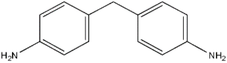
4.4’-Diaminodiphenylmethane (aniline, MDA), an aromatic diamine, is commonly used as an intermediate product for the development of MDI. In addition, MDA is used for the manufacture of polyamides, metal corrosion inhibitors, vulcanization accelerators, and hardness of epoxy resins. Figure 1 displays the MDA structural formula.

In the chemical industry the most commonly used synthesis of MDA is the reaction of aniline with formalin in the presence of hydrochloric acid under mild temperature (60–110 °C) conditions [4]. In order to prevent the use of hydrochloric acid and the formation of a significant volume of NaCl solution as a waste product, a variety of attempts have been made [5,6,7,8,9,10,11,12] to substitute current technology with a catalytic process using solid acids, zeolites, layered materials, ionic liquids or ion-exchange resins as catalysts. However, none of the methods for catalytic production of MDA have yet gone beyond the laboratory or pilot stage, making the study of the MDA obtaining process a significant challenge. However, this study is complicated by the need to carry out a large number of experimental trials, which require considerable costs and time. This problem can be overcome by designing computational mathematical models to predict the kinetics of the investigated reaction. As a result, the costs of conducting chemical reaction studies can be significantly reduced by partially replacing full-scale experiments with computational ones.

One of the current modeling methods that can be used to build models for predicting chemical reactions is the cellular automata (CA) approach. The CA approach is based on the simplification of the system, when it is represented as a set of finite automatons located in discrete cells of the spatial lattice. Each cell of a cellular automata has one of a given set of states at any given time. Thus, the examined system is presented in the form of a set of cells interacting with each other, and the CA discretizes the system both in space and in time. The cell state changes depending on the state of neighboring cells (a set of such cells is called the cell neighborhood) in accordance with the specified transition rules. This approach allows complex systems to be specified by applying simple local transition rules for each cell. This significantly reduces the complexity of calculations and allows the high-performance parallel calculations to speed up the calculation processes.

Currently, cellular automata are widely used for the modelling of different systems and processes, including porous structures formation and chemical reactions [13,14,15,16,17,18,19,20,21,22,23,24].

Since the catalyst used in the studied process has a nanoporous branched structure, the models that enable the generation of porous materials structure are of interest to this study. Aggregation models are one of those. The main idea of the aggregation model is to generate a field with individual particles with their subsequent movements and aggregation according to a certain algorithm [25,26,27].

There are two main approaches in aggregation models: Particle-cluster aggregation (PCA) and cluster-cluster aggregation (CCA).

In PCA methods, the clusterization center (a single globule) is placed in the generating field, and the remaining particles (globules) are generated one at a time and begin to move from a random point of the field. When a particle collides with a clusterization center or another particle, this particle aggregates and becomes a part of the cluster.

One of the variable parameters of the PCA models is the choice of the particle movement path. Classifying by this criterion, two models can be distinguished: The diffusion-limited aggregation and the ballistic model.

A diffusion-limited aggregation (DLA) model predicts particle motion caused by diffusion. A particle appears in a random place and moves randomly, changing the direction of motion at each step of its path [28].

One possible version of the DLA algorithm is reaction-limited aggregation (RLA). The distinction from DLA is that the aggregation of particles does not occur during each collision of particles, but depends on the given conditions, such as the energy of interaction of particles. The calculation of the aggregation probability in the RLA algorithm makes it possible to maintain constant porosity but to vary its branching structure, which is assumed to depend on various conditions of the production process [29].

The ballistic model (Ballistic particle-cluster aggregation, BPCA) is similar to the diffusion-limited aggregation model. The difference is that the movable particle travels along a straight line in a randomly selected direction until it collides with the particle and aggregates. The advantage of this model is the high computational speed, as the direction is chosen once, and the particle aggregates or goes beyond the boundaries much faster. The final structure generated by this method is denser than the one generated by DLA, because particles move along straight lines and do not simulate Brownian motion, which causes significant branching in the structure. An interesting version of the ballistic model is the ballistic particle-cluster aggregation with attraction, where the particle moves along a straight line from the point of generation to the clusterization center. This algorithm is faster than the previous one and the final structure is denser compared to BPCA, as the particles in this algorithm move to the clusterization center, which reduces the branching of the structure.

While PCA models are commonly used, they are not capable of accurately simulating the most common particle aggregation processes, such as colloid and aerosol processes. For this purpose, a cluster-cluster model is needed. The basic principle of this model is that the number of particles is determined and all of them are placed in the modeling field. All particles (clusters) move inside the field, bouncing as they reach the boundaries. When they collide with each other, the particles aggregate into one cluster, which also moves and can aggregate with other clusters [30]. These models are widely used in porous structure modelling [29].

In the diffusion model (diffusion-limited cluster aggregation, DLCA), the direction of cluster (particle) motion is randomly selected at each step of the path. When a cluster collides with the left or right field boundaries, the horizontal component of its velocity vector acquires the opposite sign. In the event of collision with an upper or lower boundary, the vertical component of the velocity vector changes accordingly. There are several possible variations of this model. For example, as in particle-cluster models, the diffusion and ballistic movements of the generated particles can be specified.

In a ballistic model (ballistic cluster-cluster aggregation model, BCCA), each particle (cluster) initially has the same speed and randomly selected direction of motion. When two clusters collide, new values of speed and movement direction are calculated, determined by their masses (the number of particles in the cluster) and velocities.

The development of the first two approaches led to the birth of intermediate algorithms—multi-particle-cluster aggregation, MultiPCA (MPCA). These algorithms include methods that are part of the PCA subgroup but are implemented with many clusterization centers.

In addition to structure formation, cellular automata are successfully used to model chemical reactions of simple inorganic molecules and complex biomolecular systems [13,20,21,22,23,31,32,33].

To model chemical reactions, CA where one cell corresponds to a certain specific concentration of reagent, can be used. In [32], the gasification of calcium carbonate was simulated from the equation:

CaCo₃ + 2HCl = CaCl₂ + H₂O

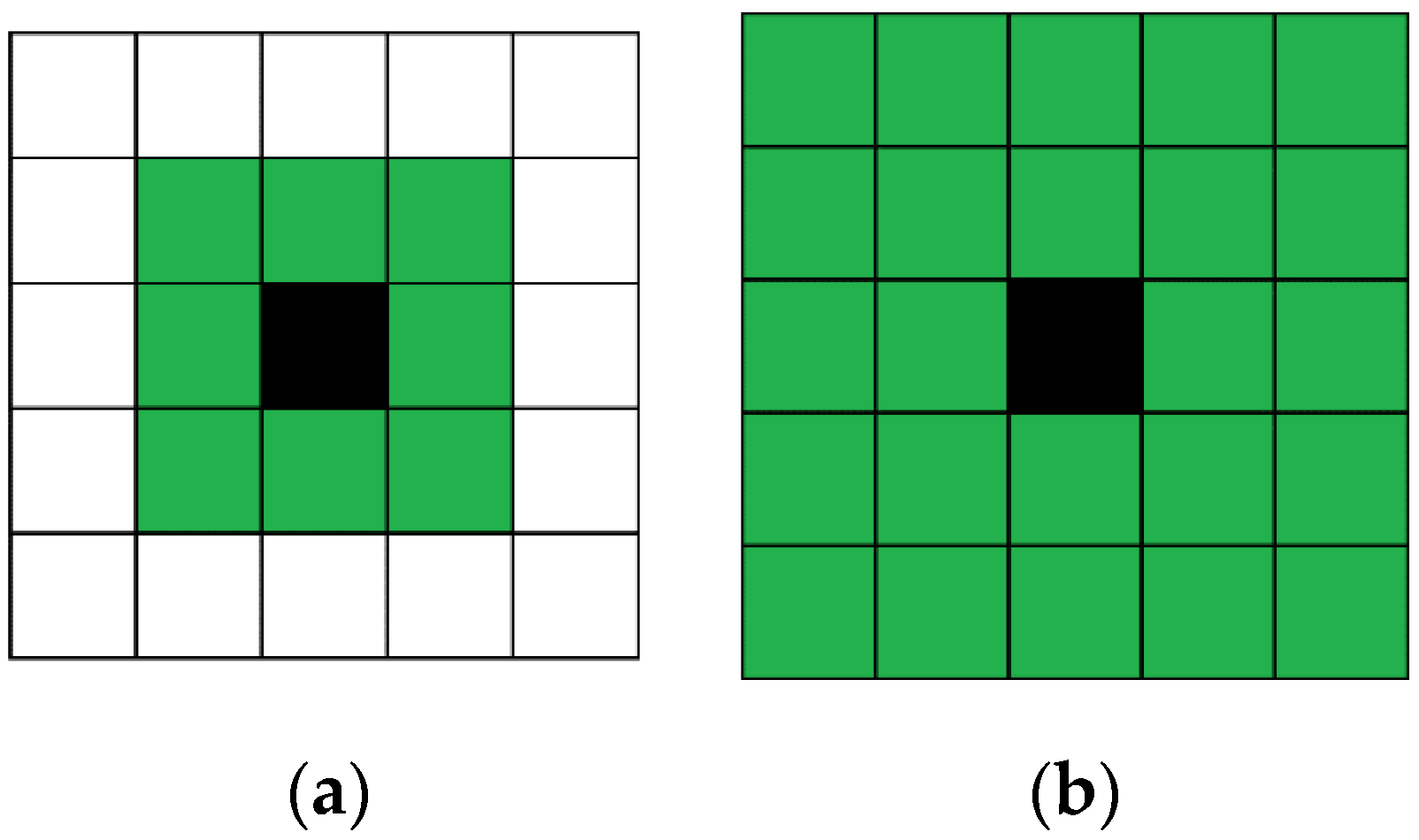
Each cell represents a certain number of reagent molecules. Cells of the automata are grouped by nine (Figure 2). In each of these regions, molecular reactions and motions are simulated. Thus, the model contains two cellular automata, the first describing the diffusion of molecules, and the second describing the reaction between them. Diffusion is modeled by changing the state of cells in each block of nine cells.

The suggested reaction automata have the following set of states S = {H2O, HCl, CaCO₃}. For reasons of simplicity and workability of the model, no additional state for the CO₂ or CaCl₂ molecules is introduced, the former because it is assumed that they escape immediately from the medium and are therefore never present in the tessellation and the latter because they are completely non-reactive dissolvable salts [34].

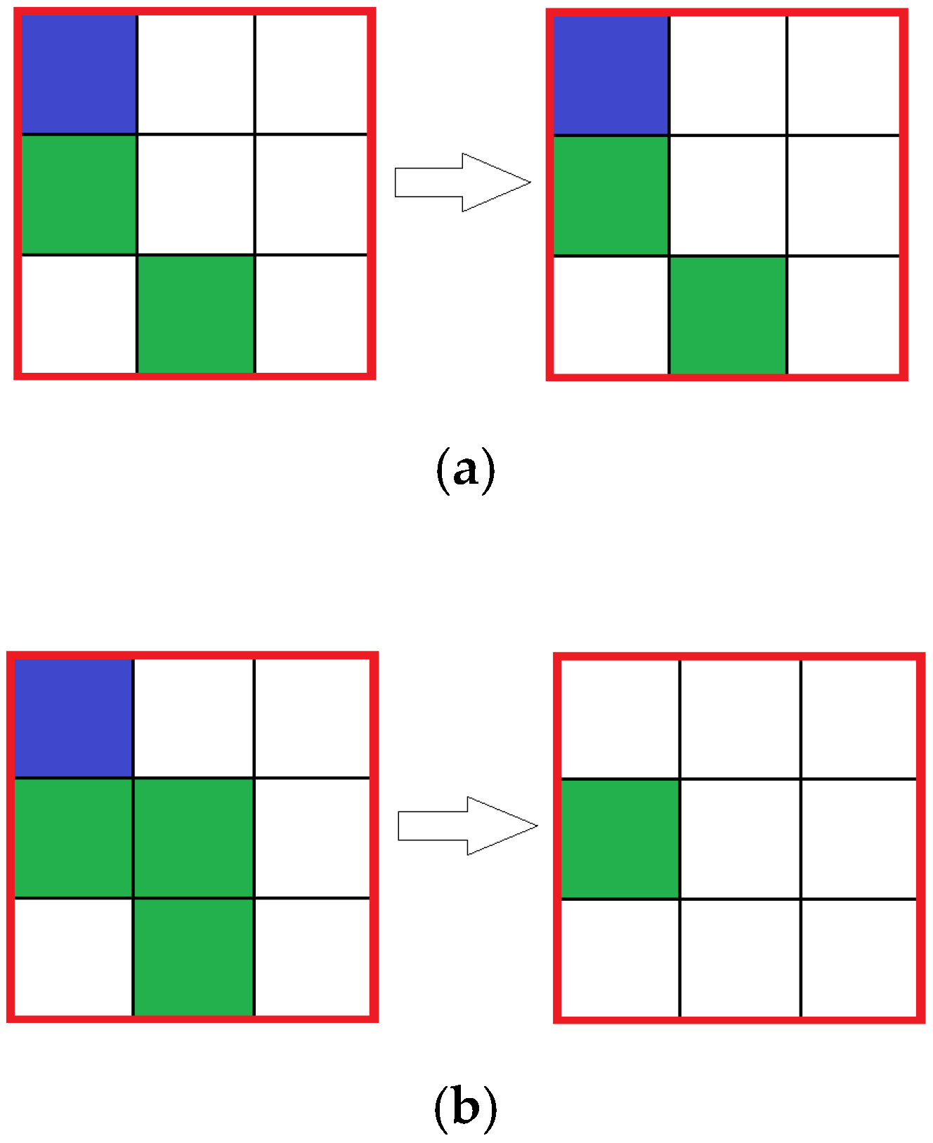
In the reaction simulating automata, the state of the central cell in each block is analyzed: if in there is a cell with solvent (water) molecules in the center cell, then the reaction does not occur, if there is either reagent 1 (HCl) or reagent 2 (CaCO₃), then the reaction occurs with a given probability, resulting in an amount of reagents inside the block to be removed corresponding to the reaction equation (Figure 3). Cells with the product do not appear, because of the assumption that the product is removed immediately.

At any moment, the number of cells of each reagent is known, so is the quantity of each reagent. Thus, the model allows the calculated kinetics curve of the reaction to be obtained, which can be easily compared with the experimental data.

This model contains unknown empirical parameters such as reaction probability. Such parameters must be selected based on available experimental data, which is a disadvantage of this approach. However, the model showed good correspondence with experimental data.

Cellular automata models that simulate catalytic reactions, in particular, reactions on the surface of a solid catalyst, are widely used and presented in a number of studies. For example, in [34] the CA approach was used to describe reactions of gas components on the surface of a solid catalyst, because of its ability to include several cellular automata with different transition rules. Therefore, it is possible to simultaneously model the processes of diffusion, adsorption, desorption, and the reaction. Another interesting example of catalytic systems modeling is [35]. The authors simulated photocatalytic decomposition of moxifloxacin on the surface of titanium dioxide. In [36], a one-dimensional cellular automata model was proposed for modeling DNA molecules.

Another interesting study is [33]. In this study, each cell corresponds to one molecule and the model describes the modelled system at the molecular level, using specific assumptions of the CA approach: Discreteness of space and time, and not taking into account the geometry of the molecule.

A current study is the development of [37]. The aim here was to combine the CA model of diffusion with the CFD modeling: by using the cellular automata model to calculate the diffusion coefficient of the system, which was then used in CFD modeling of the process of displacing aniline from a porous catalyst. The goal of the current study is the modeling of investigated reactions of obtaining MDA on the surface of the porous catalyst zeolite ZSM-5. To reach this goal, based on presented CA models, a cellular automata computer model was developed that simulates the reactor section with reagents and a porous catalyst, taking into account the influence of mixing on the reaction process. This aims to reduce the requirements for computing resources and the amount of necessary experimental data while maintaining the accuracy of sufficient calculations, and also to implement diffusion and chemical transformations within the framework of one major model, which allows for the prediction of reaction kinetics under various process conditions. In the future, the suggested model will be used with the CFD model to create a complex model of a flow catalytic reactor, which will consider both macroscale hydrodynamic effects and micro- and nano-level diffusion and chemical reactions, depending on the catalyst structure.

To model the catalytic reaction process, a cellular automata model based on the models presented in [32,33] was developed. The main assumptions for diffusion motion were taken from [28]: Particles move at each iteration within a neighborhood, and the reaction occurs when reagents and catalyst are in a certain region. At the same time, it was decided to refuse the division of the field into blocks of nine cells, applying the classical Moore neighborhood with conditions for the transition of cells from one state to another. The reaction therefore occurs not within the block, but inside the considered neighborhood of each cell that closely simulates the real process. In comparison with the model [33], it was assumed that each cell corresponds not to a certain amount of substance as in [28], but to one molecule, which also increases the accuracy of the simulation. Furthermore, in [29], it was shown that the absence of consideration of molecule geometry should not have a significant impact on the model accuracy. A detailed description of the developed model will be given in Section 3.

2. Materials and Methods

2.1. Experimental Study

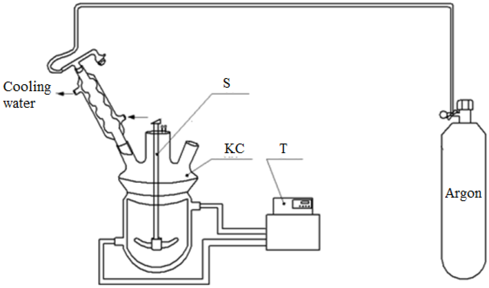
To set the empirical parameters of the model and then to estimate its adequacy, kinetic experiments were carried out using the following procedure. The experiments were carried out in a kinetic cell (Figure 4), which is a glass reactor with a jacket and a mechanical stirrer, equipped with a reflux condenser, a sampling dispenser, and a thermometer. A circulation thermostat is connected to the jacket of the reactor to create isothermal conditions in the reactor.

The kinetic experiments consist of three stages:

• Stage 1—Condensation of aniline and formaldehyde;
• Stage 2—Separation of the aqueous and organic phases and selection of the organic phase for the next 3rd stage;
• Stage 3—Catalytic rearrangement of products obtained in the 1st stage with MDA.

In stage 1, before the experiment, the reactor is purged with argon. Then, aniline is loaded into the reactor, with the stirrer and thermostat turned on. After reaching the target temperature in the reactor, a required amount of formalin is added to the reactor via a septum with a syringe, followed by a required amount of hydrochloric acid by a sampling doser, and the timer is started. The reaction time is at least 90 min. The degree of conversion of formaldehyde is determined by the residual formaldehyde content in the aqueous layer after settling (in stage 2).

At stage 2, the reaction mass following stage 1 is transferred to a separatory funnel with a jacket connected to a circulating thermostat. In the separatory funnel, the reaction mass is stratified into two layers: Aniline (lower) and water (upper). The sedimentation is carried out for 5–6 h at 40 °C to achieve residual water content in the aniline layer of not more than 3%. The completeness of the reaction is controlled by the formaldehyde content in the aqueous layer. The formaldehyde content is determined by titrimetric method. The residual formaldehyde content in the wastewater should not be more than 0.3 g/L, which corresponds to 99.95% formaldehyde conversion. Then, the aniline layer is selected and used for kinetic studies in stage 3.

The experiments of stage 3 are carried out in the same kinetic cell as in stage 1. Before the experiment, the reactor is purged with argon. Then, the aniline layer obtained in stage 3 is loaded into the reactor, with the stirrer and thermostat turned. After reaching the target experiment temperature in the reactor, a catalyst sample is charged through the throat of the reactor and the timer is started. The used catalyst, zeolite ZSM-5, is a granule of cylindrical shape with a color ranging from white to beige. The diameter of the granules is 1.5–2 mm and the length is 5–20 mm. The granules have porous structure, with channel pore size of about 5.4–5.6 Å.

During the experiment, sampling in accordance with the schedule of control points of the experiment and a quantitative analysis of the composition of the reaction mass by HPLC were carried out.

Experimental studies were carried out under atmospheric pressure. The main parameter that affects the rate of a chemical reaction is temperature; therefore, at stage 3 of kinetic studies, it is necessary to control the temperature. The required temperature is set using the thermostat and is controlled by a thermometer. Since heterogeneous catalysts are used in step 3, it may be necessary to provide a reaction in kinetic mode by maintaining a certain range of speed of the mixer. Therefore, the speed of the mixer should be a controlled parameter. To control the speed of revolutions of the mixer, a laboratory mixer with adjustment and a speed sensor is used. At stage 2 of the kinetic studies (separation of the aniline and water layers), it is necessary to control the residual water content in the aniline layer of not more than 3%.

Since the formation of the target product (MDA) proceeds at stage 3 of the experiment, for the planning of kinetic studies, variable parameters that affect the course of the respective reaction at the third stage are selected. Since heterogeneous catalysts are used at stage 3 of kinetic studies, it may be necessary to provide a reaction in kinetic mode by maintaining a certain range of speed of the mixer. To determine such range, it is necessary to conduct a series of experiments for each catalyst at different mixer speed. The proposed speed range of the stirrer is 300–500 rpm.

According to the law of masses, the rate of a chemical reaction depends on the concentrations of the reagents and the catalyst. In this regard, it is necessary to conduct a series of experiments with varying initial concentrations of reagents (aniline and formaldehyde) and concentrations of the catalyst. The concentration of reagents will be varied by changing the initial molar ratio of aniline: formaldehyde in step 1. The reaction was carried out with a molar excess of aniline, with a variation in the molar ratio of aniline: formaldehyde in the range from 4 to 6.

According to the Arrhenius equation, the rate constant of a chemical reaction exponentially depends on temperature, therefore, for the temperature in step 3, the following ranges of variation were selected: 50–130 °C.

Summarizing the above, the following experimental parameters were selected:

• The temperature during the kinetic studies of stage 3 was varied with a step of 20 °C; therefore, in the range of 50–130 °C, experiments were carried out at five temperatures: 50, 70, 90, 110, and 130 °C.
• The experiments were carried out at five different speeds of the mixer in the range of 300–500 rpm, 300, 350, 400, 450, and 500 rpm.
• The initial molar ratio of aniline: formaldehyde.
• The experiments were carried out at three values of initial molar ratio of aniline:formaldehyde: 4, 5, and 6.
• The experiments were carried out at four catalyst concentrations: 40, 80, 120, and 160 g per kg of aniline layer.

All data, including the reaction conditions and key parameters, are given in summary

Table 1. Conditions of Experiments.

Experiments Series	Catalyst Concentration, g per Aniline Layer kg	Temperature, °C	Aniline: Formaldehyde Ratio	Stirrer Speed, Rpm
C 1.1, 1.2, 1.3	40	130	5	300
C 1.4	40	130	5	350
C 1.5	40	130	5	400
C 1.6	40	130	5	450
C 1.7, 1.8, 1.9	40	130	5	500
C 2.1, 2.2, 2.3	40	110	5	500
C 2.4	80	110	5	500
C 2.5	120	110	5	500
C 2.6, 2.7, 2,8	160	110	5	500
C 3.1, 3.2, 3.3	40	110	4	500
C 3.4	40	110	5	500
C 3.5, 3.6, 3.7	40	110	6	500
C 4.1, 4.2, 4.3	40	50	5	500
C 4.4	40	70	5	500
C 4.5	40	90	5	500
C 4.6	40	110	5	500
C 4.7, 4.8, 4.9	40	130	5	500

.

For these experiments, kinetic curves were obtained and later used in the computational experiments to simulate chemical reactions.

2.2. Modelling

Two models were used in the current study: A model for generating a digital catalyst structure and a model of catalytic reaction on its surface.

2.2.1. Catalyst Digital Structure Generation

The used zeolite ZSM-5 catalyst has a branched porous structure with pore sizes of 5.4–5.6 Å. The digital structure of such samples is successfully generated using the aggregation models given in Section 1. As the aggregation model, the MultiDLA model was chosen using the cellular automata approach. This model belongs to the class of PCA aggregation models and is an extension of the diffusion-limited aggregation (DLA) model. As in any PCA model, in DLA, a stationary particle is placed on the field, which is the center of clustering, and other particles moving in field aggregate with it, forming a single branched cluster. A feature of DLA is that it models the motion of a particle caused by diffusion. A particle appears in a random place and moves randomly, changing the direction of motion at each step of its path [26]. Aggregation models are successfully implemented using the cellular automata approach, since the locality of the CA transition rules combines well with the representation of the system in the form of many independent interacting particles.

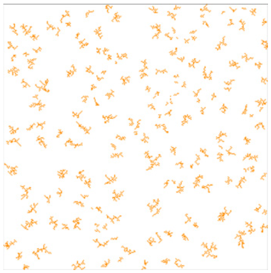
The MultiDLA model used in this work differs from the DLA because not a single, but several fixed clusterization centers are placed on the field. This allows for the obtaining of a branched and uniformly distributed porous structure [38]. Figure 5 shows a two-dimensional slice of the digital catalyst structure generated using the MultiDLA model.

The value of porosity, i.e., the ratio of empty cells to catalyst cells, is used as an input parameter. This parameter characterizes the amount of catalyst in the simulated space. In addition, the number of clustering centers is used as input parameters.

This model was chosen because it allows the branching of the structure to be controlled by input parameters of the model (the number of clustering centers).

2.2.2. Chemical Reactions Modelling

In the studied process, two independent mechanisms can be distinguished—the reaction on the surface of the catalyst and the movement of the substance under mixing. For each of these processes, two cellular automata were developed.

• The following assumptions apply to both automata in the developed model:
• The size of all molecules is equal to 1 nm.
• The size of one cell corresponds to 1 nm.
• Molecule geometry is not considered.
• Intermediate reactions are not considered—as a result of formaldehyde-aniline reaction “product” is synthesized. “Product” is the complex of 3 resulting substances: 4,4′-MDA; 2,2-MDA; 2,4-MDA.
• The size of the modelled reactor local area is 300 nm.

The developed cellular automata model consists of two cellular automata: One of them models the movement of substances (motion automata), and the second one models a chemical reaction (reaction automata). For both automata, cells can take the same set of values corresponding to the substances involved in the reaction: “aniline”, “formaldehyde”, “catalyst”, “product”, and “solution”. One cell corresponds to one molecule. The boundary conditions are toroidal for both automata.

Motion Automata

The general principle of the developed automata is as follows: a substance (“aniline”, “formaldehyde”, and “product”) can move into any free cell (a cell with the “solution” state) within a given neighborhood with equal probability. For example, if a cell has 4 free neighbor cells, the probability of this cell moving in each of its neighbors is 0.25.

Automata uses Moore neighborhood with a different order. For example, the cell has 8 and 24 neighbors for the 1st and 2nd order Moore neighborhood, respectively (Figure 6). Different order allows the distance which a substance can pass during one-time step to be adjusted. Automata is asynchronous, so cells move one after another. Each cell is chosen randomly, but the cell that has already moved during the current time step is static.

The field with a porous catalyst is the input parameter of the model, and its structure is obtained using the model described in Section 2.2.1. In addition, another input parameter is the size of the neighborhood, that is, the distance over which the cell with the substance can move. This parameter characterizes the stirrer speed and is empirical, that is, its value for each real stirrer speed should be established on the basis of available experimental data.

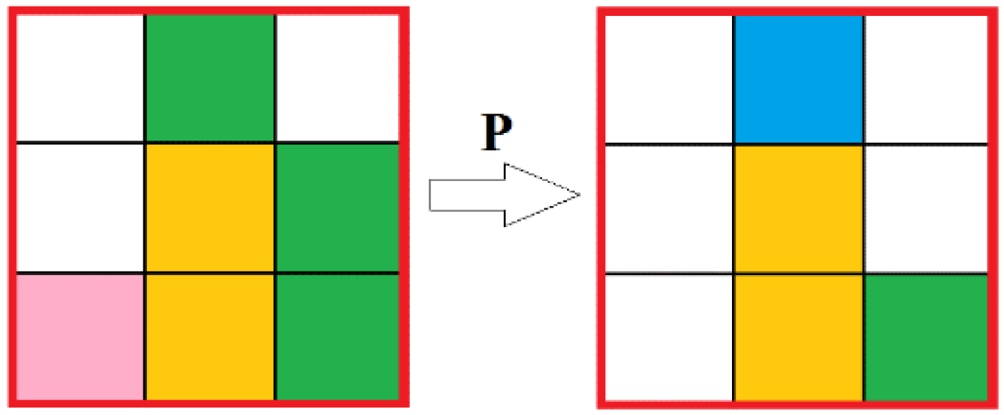
Reaction Automata

The general principle of the automata is as follows: The neighborhood of each cell is checked for the presence of a certain ratio of reagents (“aniline” and “formaldehyde”) and catalyst. If there is the required number of reagent cells and at least one cell with the “catalyst” state inside the neighborhood, then a “reaction” occurs with a certain predetermined probability p, that is, the reagents are removed in the required ratio, and a random free cell in the neighborhood is set in the “product” state. For the current reaction, the required ratio of reagents is 2 aniline and 1 formaldehyde which corresponds to the real process (Figure 7).

The automata are asynchronous, that is, the new state is calculated in a random order, so the calculation of the states of the subsequent cells takes into account the new state of the previous cell. This is done in order to avoid a situation when the same cell enters into several reactions with a substance. The automata use the 1st order Moore neighborhood.

The input parameter of the model is a field with a porous catalyst. The structure of the catalyst is generated using the model described in Section 2.2.1. In addition, the input parameter of the model is the probability of a reaction in the presence of catalyst, which allows for different reactivity of substances and the number of reagents (aniline and formaldehyde) to be simulated. The number of reagents can be obtained from the experimental data; the reactivity value is an empirical parameter.

Figure 8 shows several stages of the evolution of the catalytic reaction cellular automata.

Mathematically developed CA-model can be described as follows:

$$U=A,X,\theta ,S,$$

where

• $A=\left\{u:u=\left\{a,b,c,d,e\right\}\right\}$, a—“aniline”, b—“formaldehyde”, c—“catalyst”, d—“product”, e—“solution”
• $X=\left\{x:x=\left(i,j\right)\right\}$—set of cell names (coordinates)
• $\theta \left(x\right)=\Phi \left({\theta }_1\left(x\right),{\theta }_2\left(x\right)\right)$—combined local operator
• $S\left(x\right)=\left\{(u_0,x),(u_1,{\phi }_1\left(x\right),\dots {\phi }_k\left(x\right))\right\}$—neighborhood; k = (2n+1)²−1, where n is neighborhood order;

${\theta }_1\left(x\right)$ is motion local operator. It is applied to cells $(u_0,x)$ and replaces states with one of neighbor cells:

${\theta }_1\left(x\right):\left((u{\prime }_0=u_e)\&(u{\prime }_e=u_0)\right), if \frac{e}{k}\le p_m<\frac{e+1}{k}$

where e = 0, 1, ..., k−1;$p_m$—random value, $u{’}_0$, $u{’}_e$—new states of cells.

${\theta }_2\left(x\right)$ is reaction local operator. It is applied to cells $(u_0,x)$ and changes states of $(u_0,x)$ and neighbor cells:

${\theta }_2\left(x\right):\left((u{\prime }_e=e)\&(u{\prime }_r=e)\&(u{\prime }_t=e)\&(u{\prime }_g=d)\right), if \left(\left((u_e=b)\&(u_r=a)\&(u_t=a)\right)\left|\left((u_e=a)\&(u_r=b)\&(u_t=a)\right)\right|\left((u_e=a)\&(u_r=b)\&(u_t=b)\right)\&(u_g\ne c)\&p_m\le p\right)$, where $e,r,t,g=0,1\dots k-1;e\ne r\ne t;$$p_m$—random value, p—reaction probability.

Each of the automata operates in turn, at first all the cells of the substances move, and then a reaction occurs between them. The output parameter of the model is a kinetic curve that shows the amount of product at each moment in time. This parameter can be converted to the concentration of the substance in the reactor, which allows the calculated and experimental kinetic curves to be compared.

The suggested model simulates a reaction process between aniline and formaldehyde in the presence of the catalyst with the specified assumptions. This model uses only experimental (reagents ratio) and model (reaction probability, motion distance) parameters. So, the model does not require any complex calculations but only needs to estimate model parameters. In [28], the same approach was used in CA-modelling of chemical reaction. The model also used only experimental and model (such as reaction probability) parameters. This work showed the possibility of using the CA approach in chemical reaction modeling and a comparison of CA-model results with differential equations of kinetics and Arrhenius equation. Therefore, [28] model and models suggested in the current work are simulation models, but they can be applied for systems, described through differential equations of kinetics and the Arrhenius equation.

3. Results and Discussion

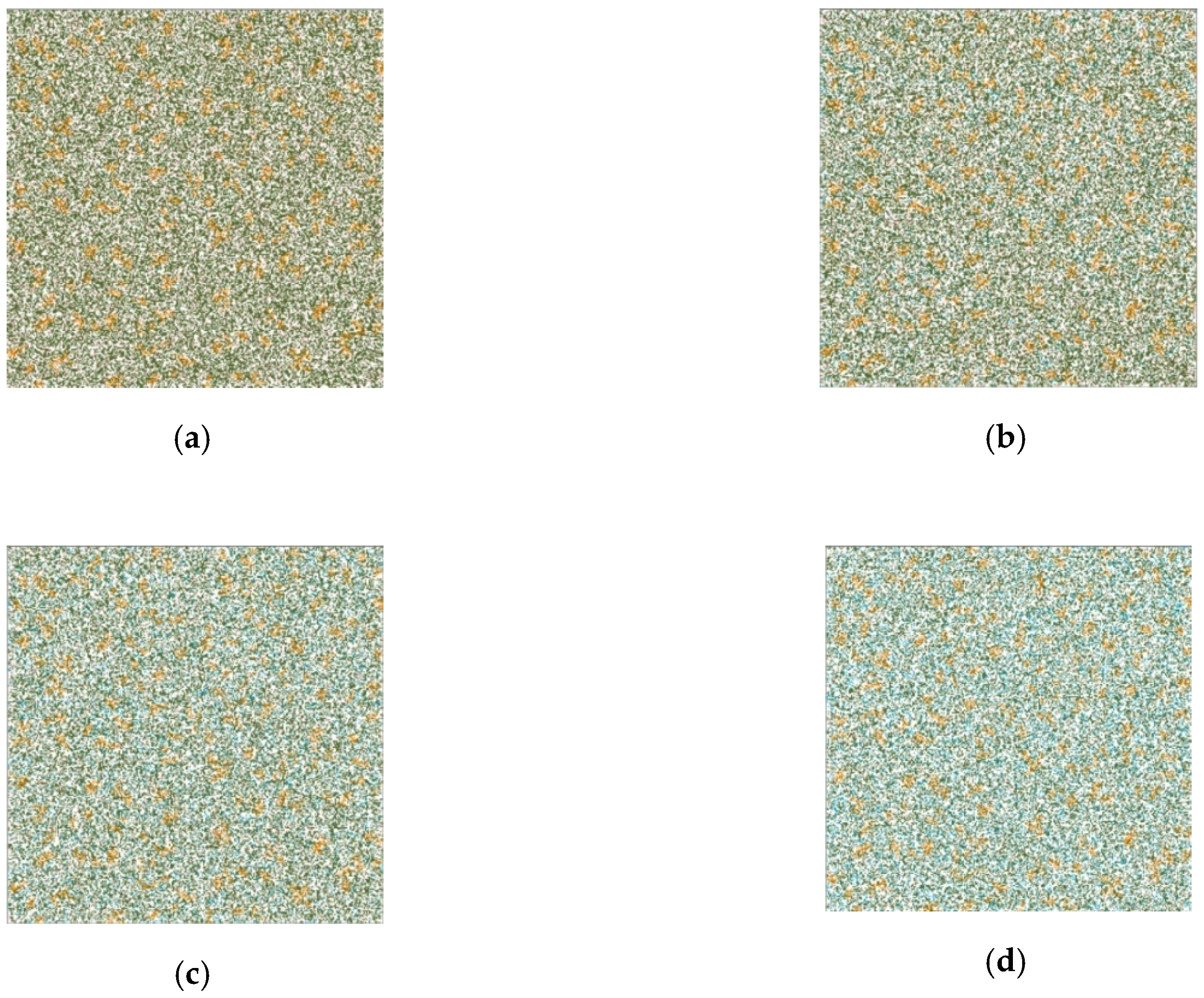
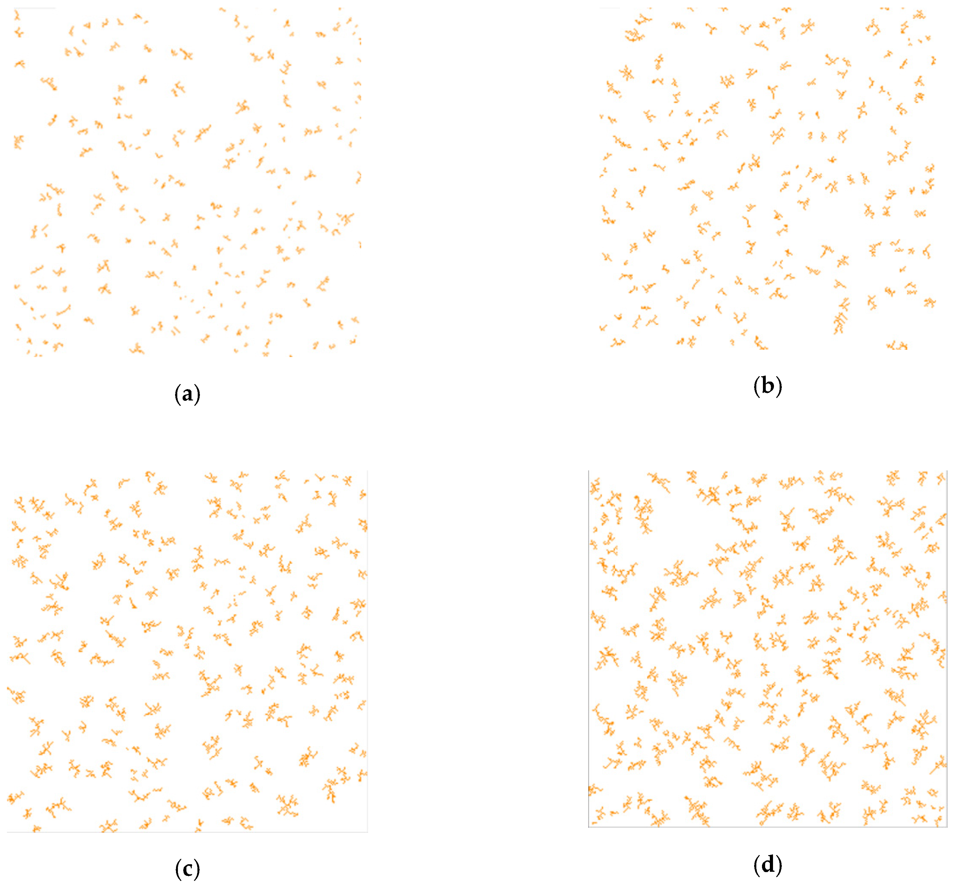
One of the main input parameters of the catalytic reaction model is the digital structure of the porous catalyst. The porosity of the structure can be obtained from the experimental conditions. The number of cluster centers was set as 5% of the total number of cells with a catalyst, which allows a branched structure to be generated. In the studied reactions, the following catalyst ratios were used—40, 80, 120, and 160 g per 1 kg of aniline layer. In accordance with these data, four three-dimensional digital porous catalyst structures were generated using the model described in Section 2.1. Figure 9 shows two-dimensional slices of these structures.

The developed reaction model contains a number of empirical parameters and their value should be defined: The probability of reaction and the order of the automata neighborhood. The first parameter characterizes the reactivity and depends on temperature, and the second one characterizes the stirrer speed. To establish these parameters a series of computational experiments were carried out in which these parameters were varied. The obtained calculated kinetic curves were compared with the selected experimental curves (the reference ones).

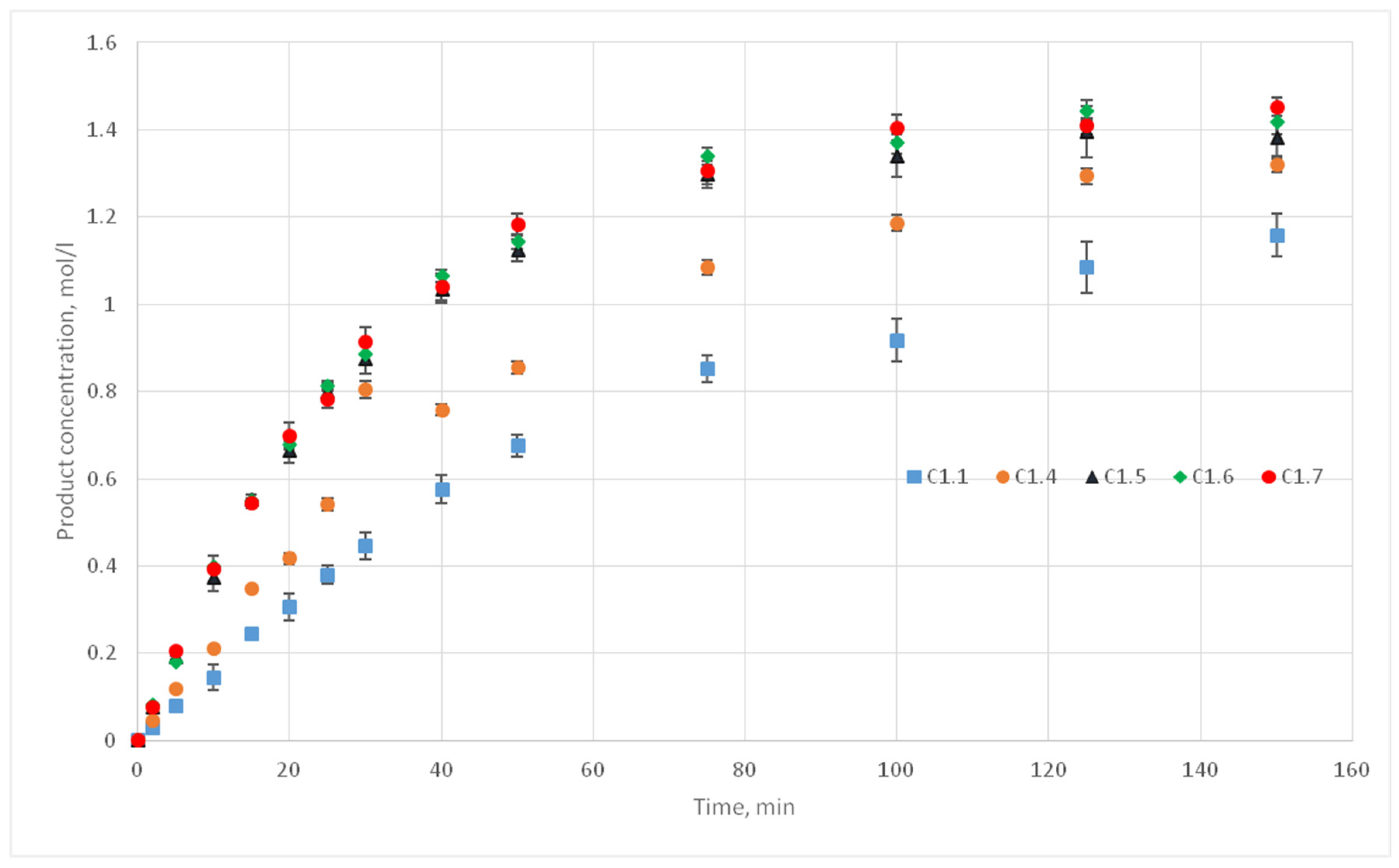
The experiments of the C1 series were chosen as reference curves, since they were carried out at the same temperature of 130 °C, and only the stirrer speed was varied from 300 to 500 rpm. Therefore, in the simulation, the reactivity parameter will not vary, only the distance of cells movement per iteration time will vary. The experimental conditions of the C1 series are presented in

Table 2. C1 Series Experimental Conditions.

Experiments Series	Catalyst Concentration, g per Aniline Layer kg	Temperature, °C	Aniline: Formaldehyde Ratio	Stirrer Speed, rpm
C 1.1, 1.2, 1.3	40	130	5	300
C 1.4	40	130	5	350
C 1.5	40	130	5	400
C 1.6	40	130	5	450
C 1.7, 1.8, 1.9	40	130	5	500

, and Figure 10 shows the corresponding kinetic curves with the confidential intervals for each experimental point. For each experiment (C1.1, 1.2, 1.3; C1.4; C1.5; C1.6; C1.7, 1.8, 1.9) three kinetic curves were obtained.

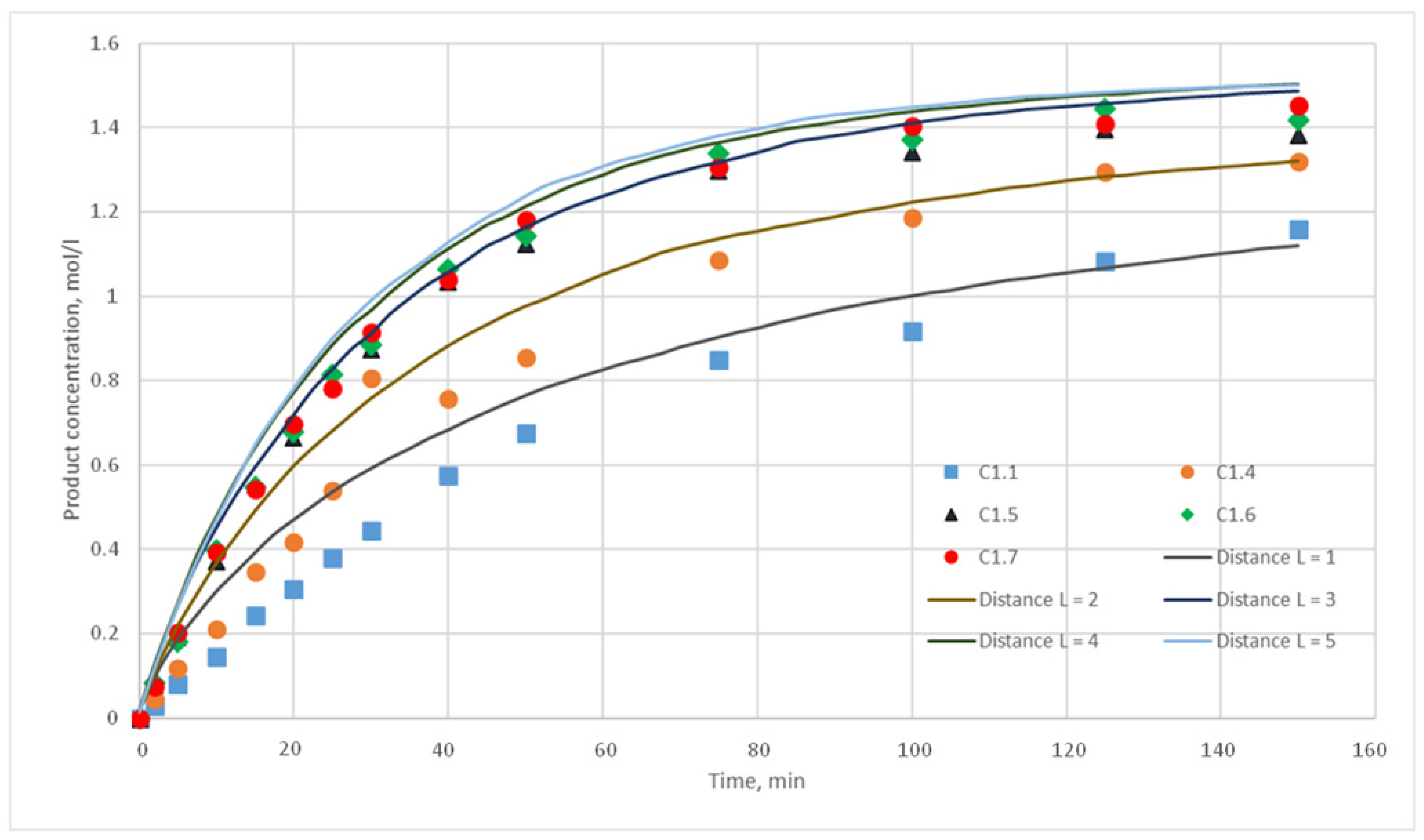
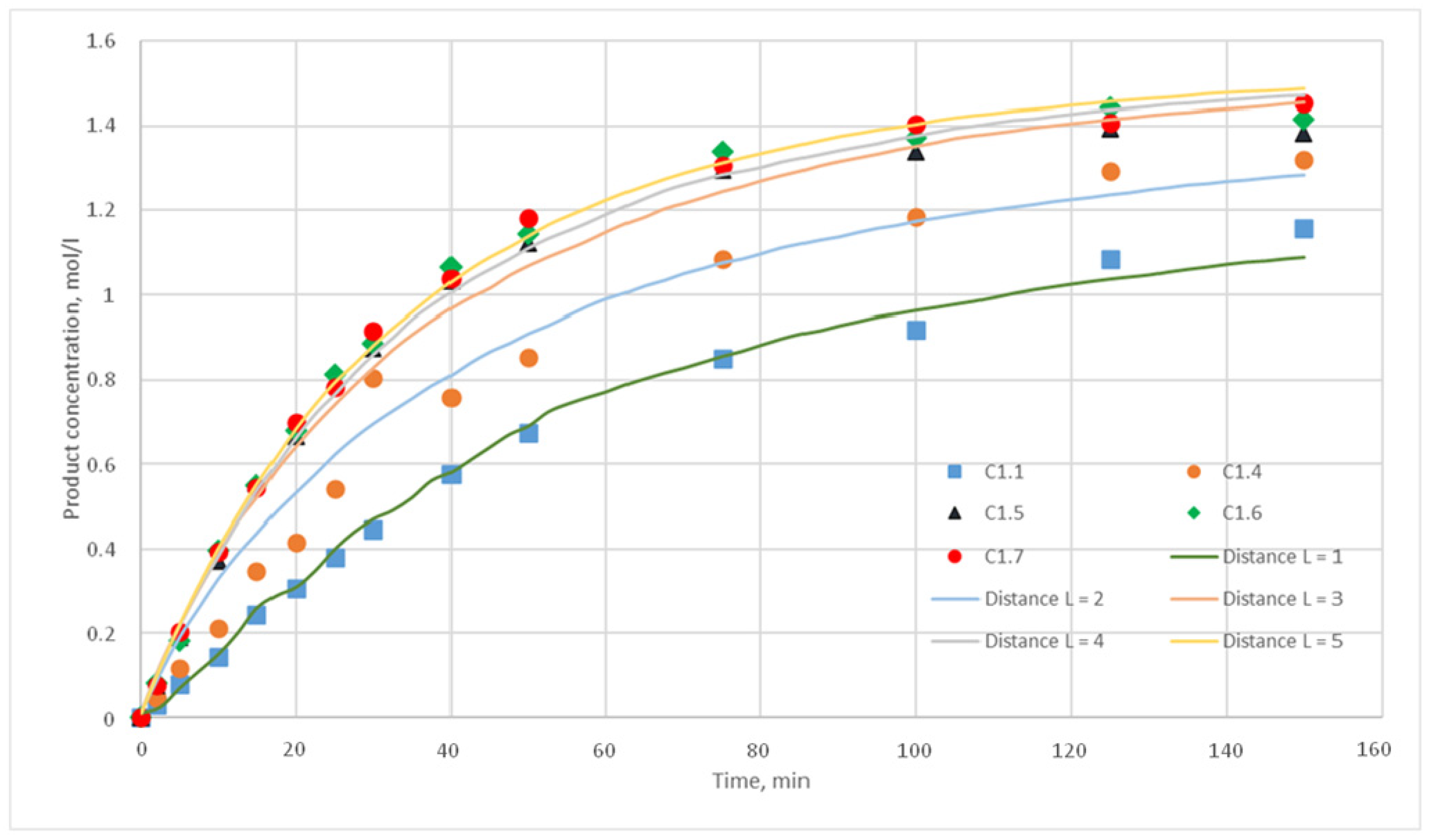
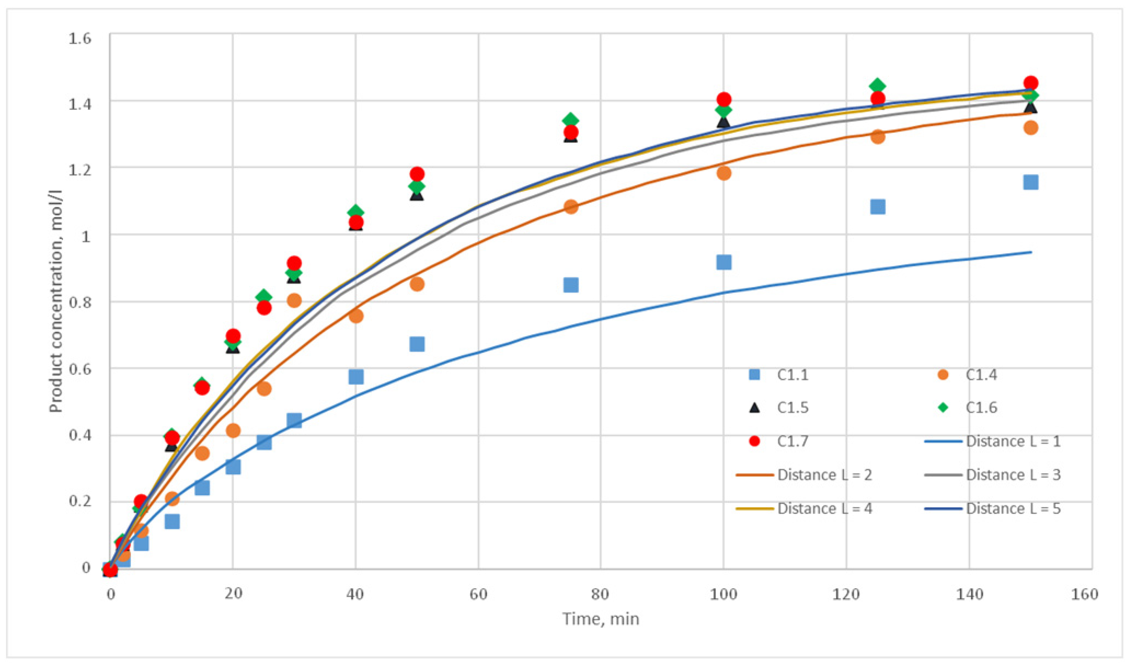
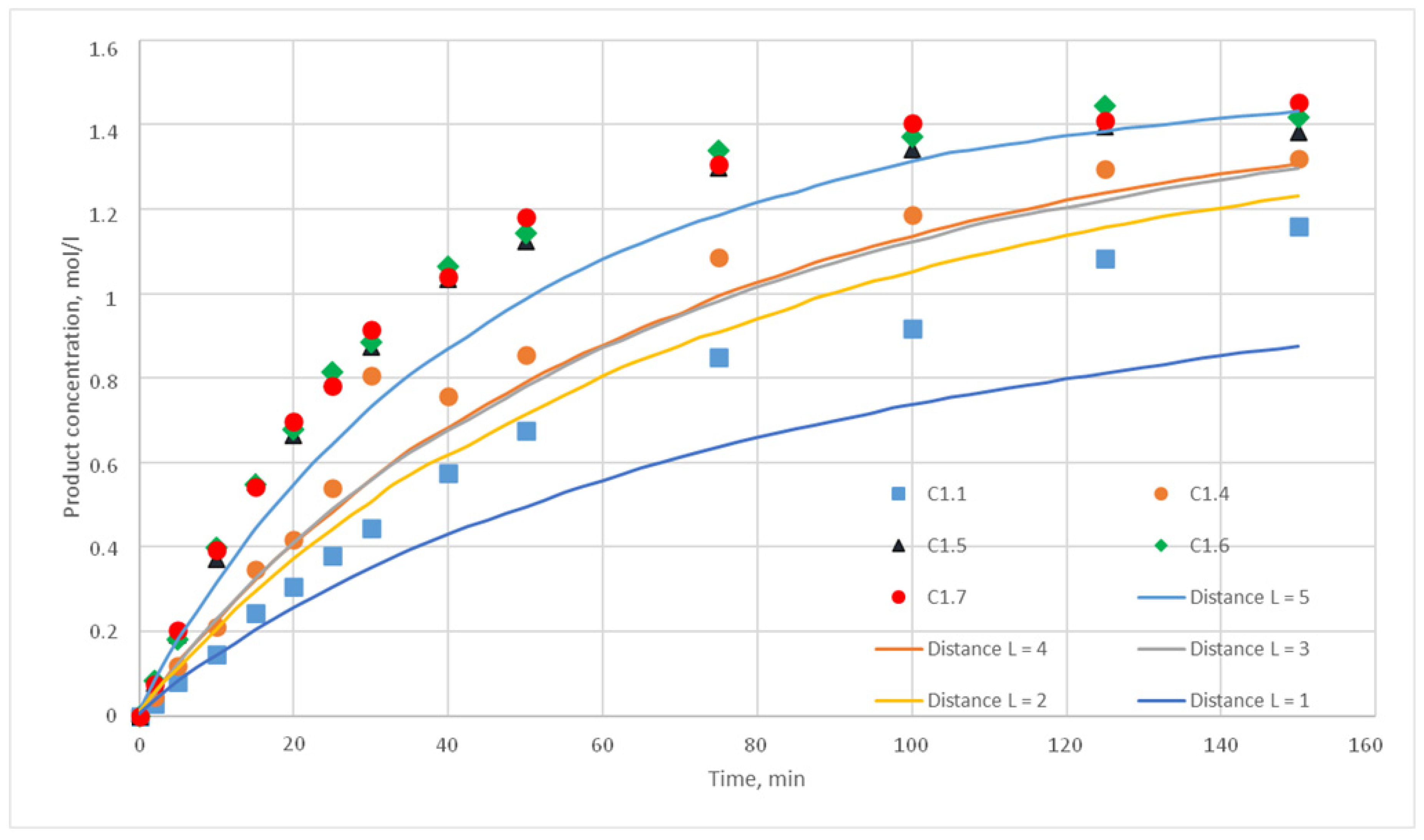
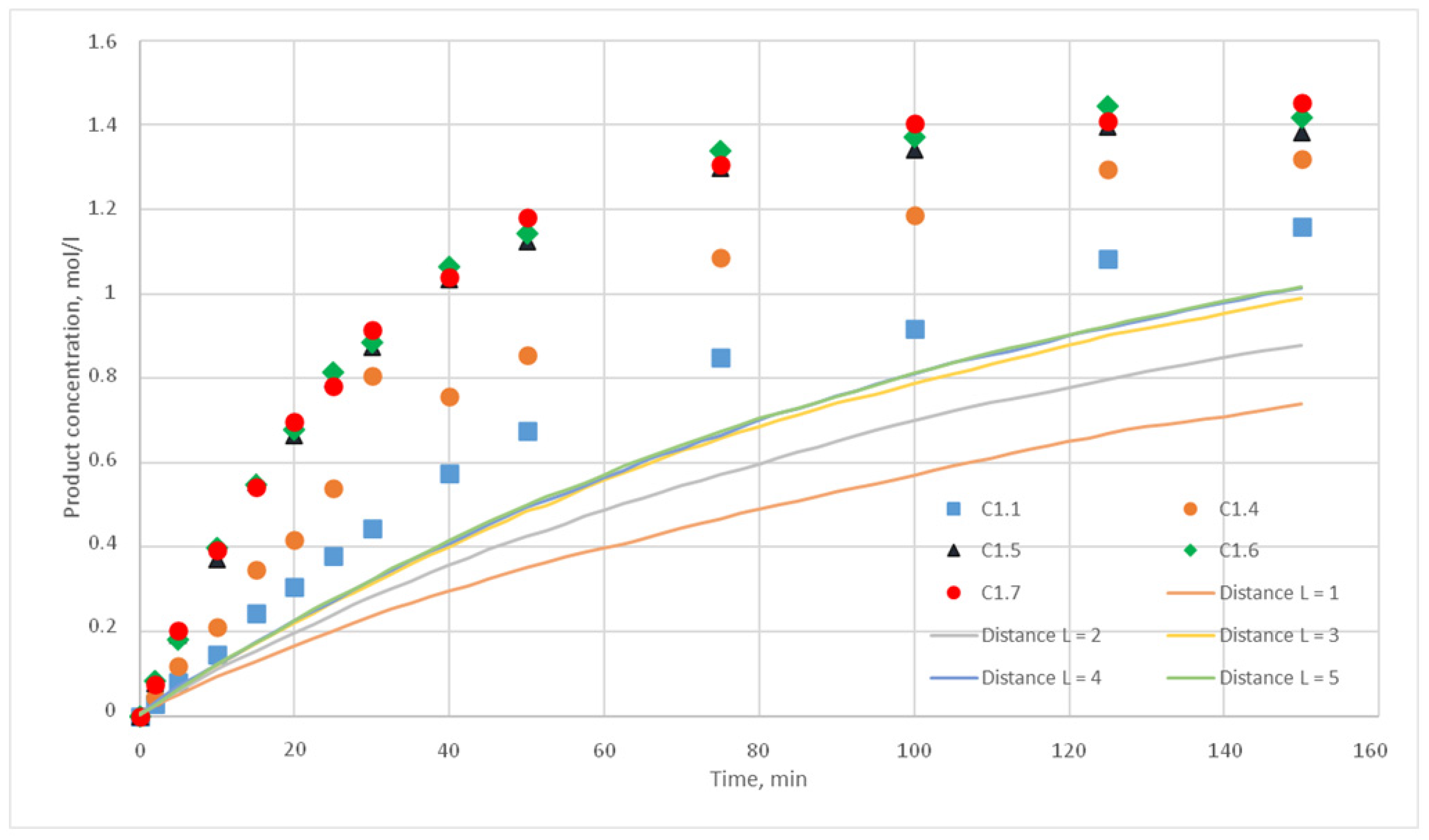
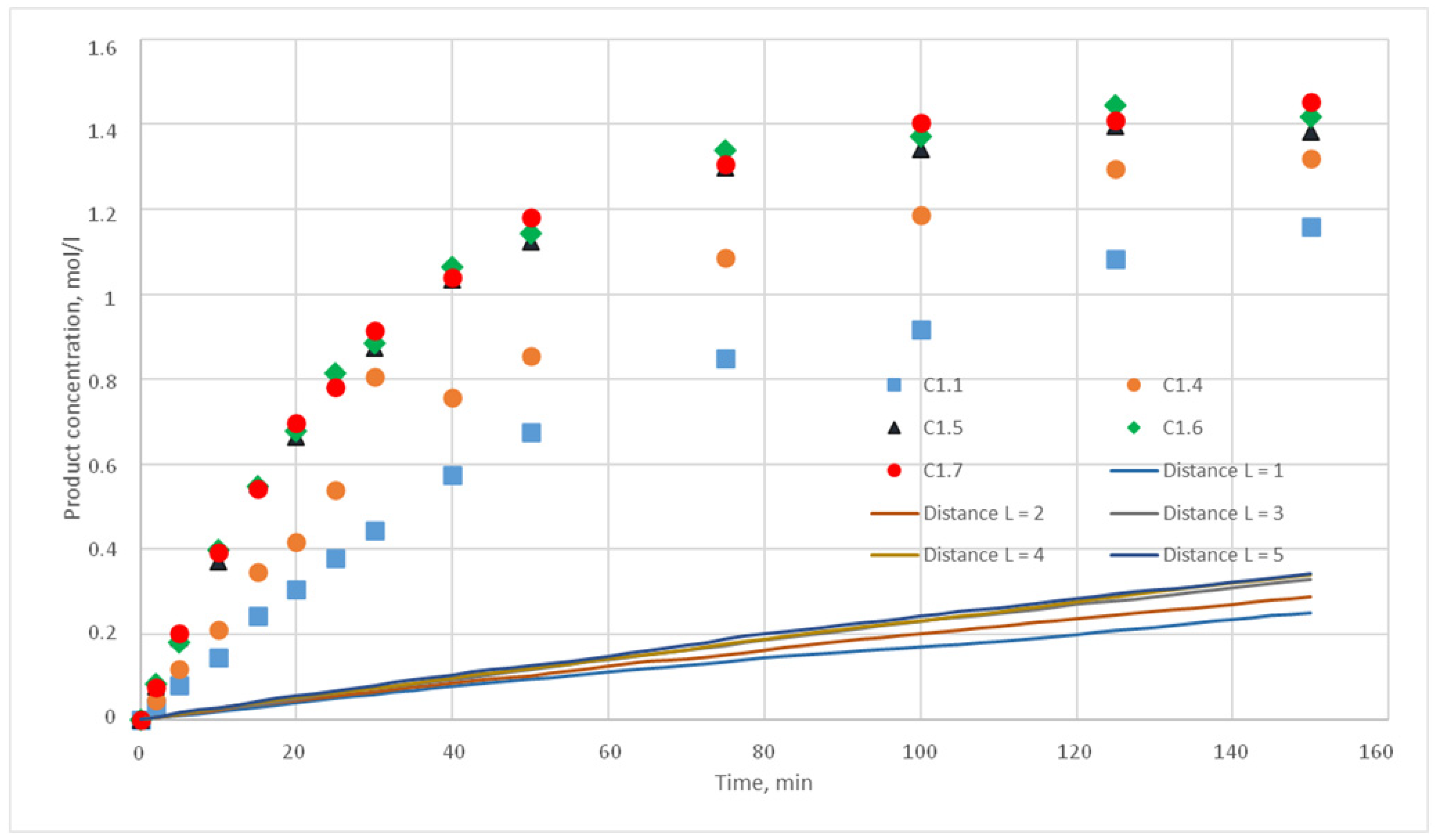
The reaction probability p characterizes the number of reactions that must occur in suitable conditions of given reaction (location nearby a given ratio of cells of reagents and the presence of a catalyst). For computational experiments, the values p = {0.025; 0.020; 0.015; 0.010; 0.005; 0,001} were chosen. For each of these values, the distance L of the motion of the substance cells during the motion phase was varied. For this distance, the following values were taken, L = {1; 2; 3; 4; 5}. Such values were chosen, as during test calculations it was revealed that a value L above 5 does not have any effect on the calculated kinetic curve. Thus, 30 computational experiments were carried out, and respective calculated kinetic curves were obtained. Figure 11, Figure 12, Figure 13, Figure 14, Figure 15 and Figure 16 present the calculated and experimental kinetic curves.

The value for the reaction probability p should be selected as the value corresponding to the smallest deviation of the calculated curves from the experimental curves. For the temperature of 130 °C, this value is 0.020. With such a p value, curves with different distances of L have the smallest deviation from the experimental ones. In addition, L values corresponding to various values of the stirring speed were obtained. Thus, for 130 °C in the developed model, the probability of reaction p is 0.020, and the values of L are 1, 2, 3, 4, and 5 for stirring speed of 300, 350, 400, 450, and 500 rpm, respectively. With these parameters, the deviation of the calculated curves from the experimental curves of the C1 series experiments does not exceed 14%.

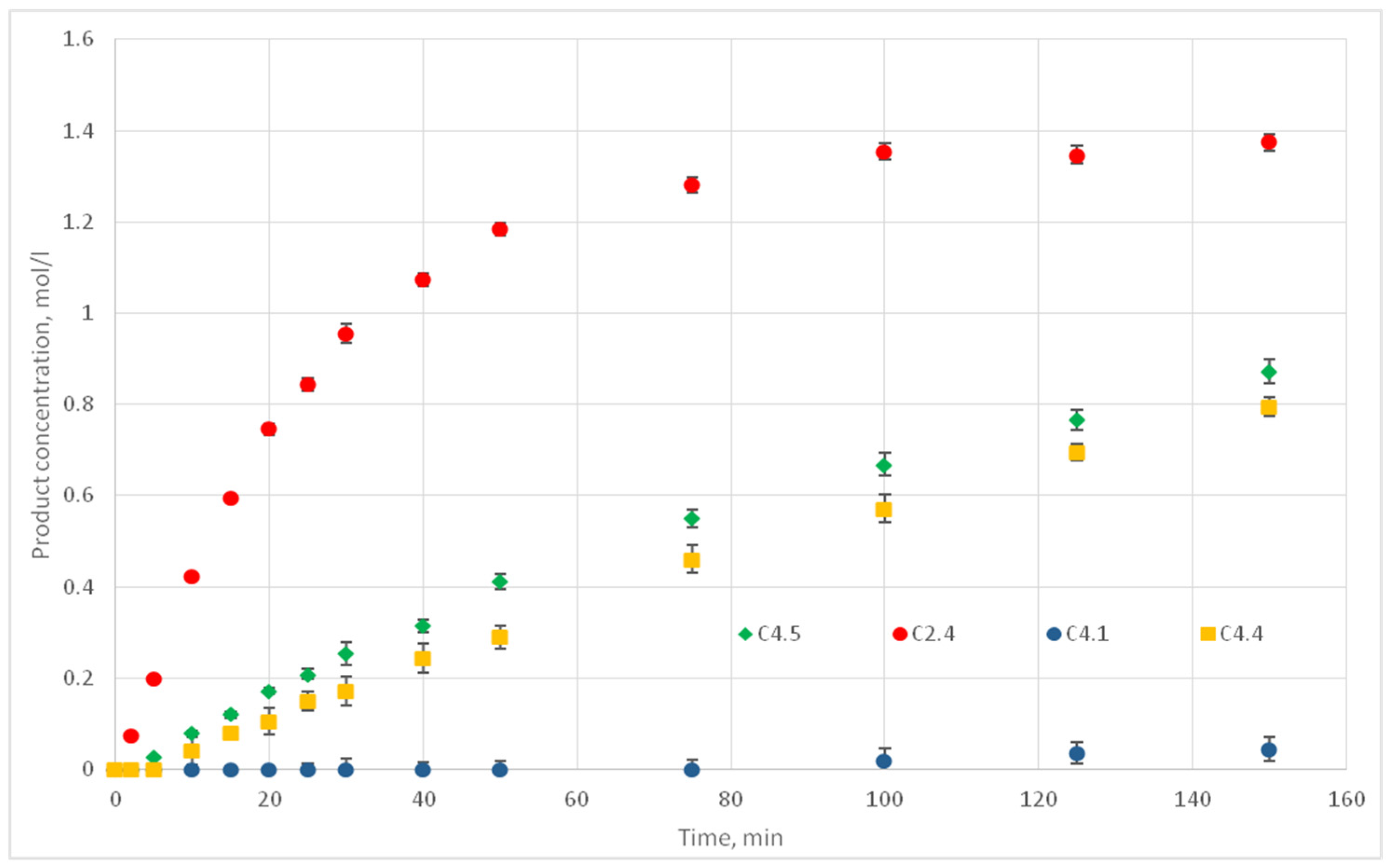
After L values were identified, the values of P corresponding to other temperatures were similarly found: 50, 70, 90, and 110 °C. For these temperatures, the kinetic curves of experiments C 4.1, C 4.4, C 4.5, and C 2.4 were used as reference curves.

Table 3. C4.1, 4.4, 4.2 и 2.4 Experimental Conditions.

Experiments Series	Catalyst Concentration, g per Aniline Layer kg	Temperature, °C	Aniline: Formaldehyde Ratio	Stirrer Speed, rpm
C 4.1	40	50	5	500
C 4.4	40	70	5	500
C 4.5	40	90	5	500
C 2.4	80	110	5	500

shows the conditions, and Figure 17 shows the kinetic curves of the experimental data.

For the temperature values of 50, 70, 90, and 110 °C the reaction probability values of p are 0.001, 0.006, 0.008, and 0.012, respectively. Thus, all the necessary input data for the operation of the model were obtained. Computational experiments were carried out to predict kinetic curves and their comparison with the experimental curves.

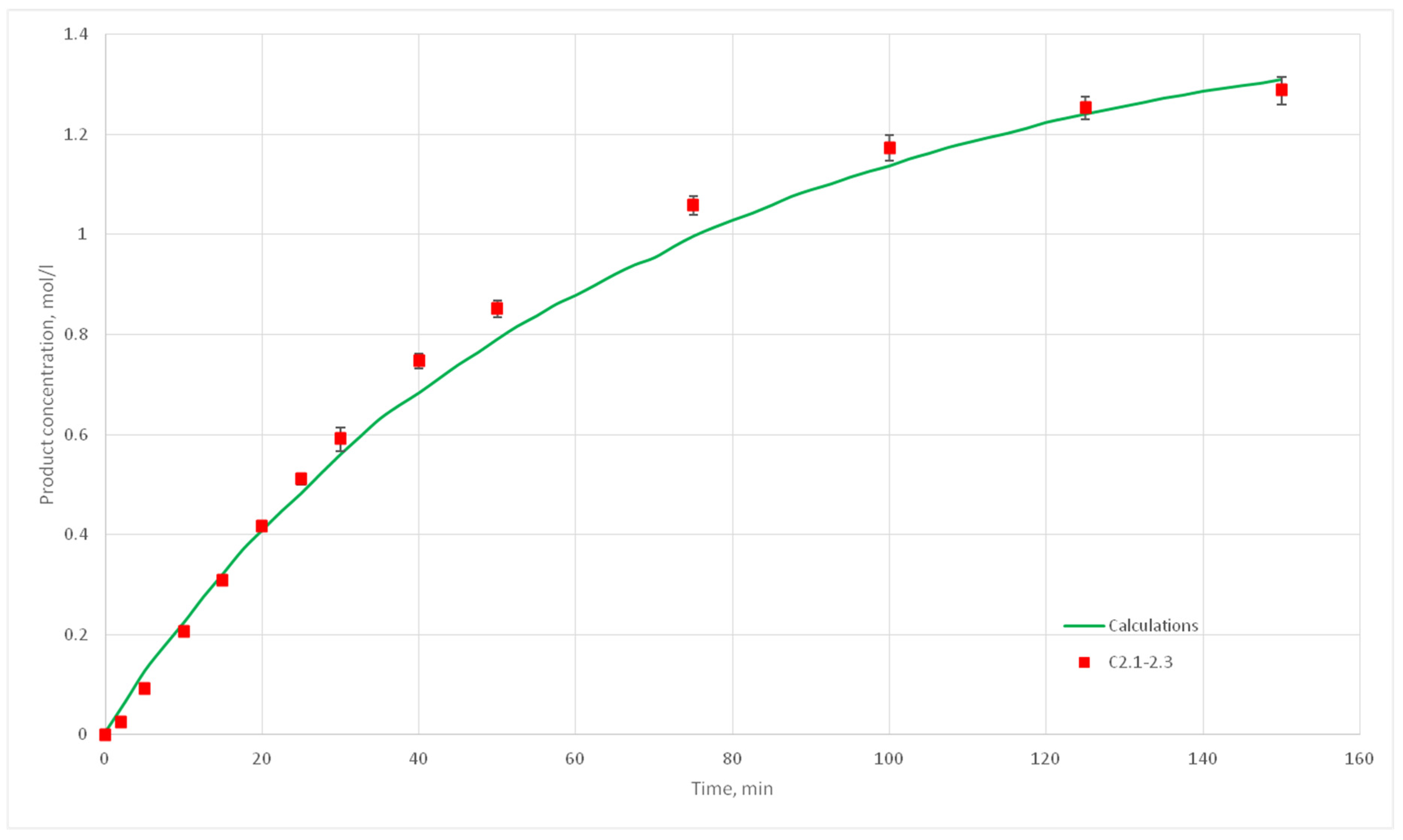
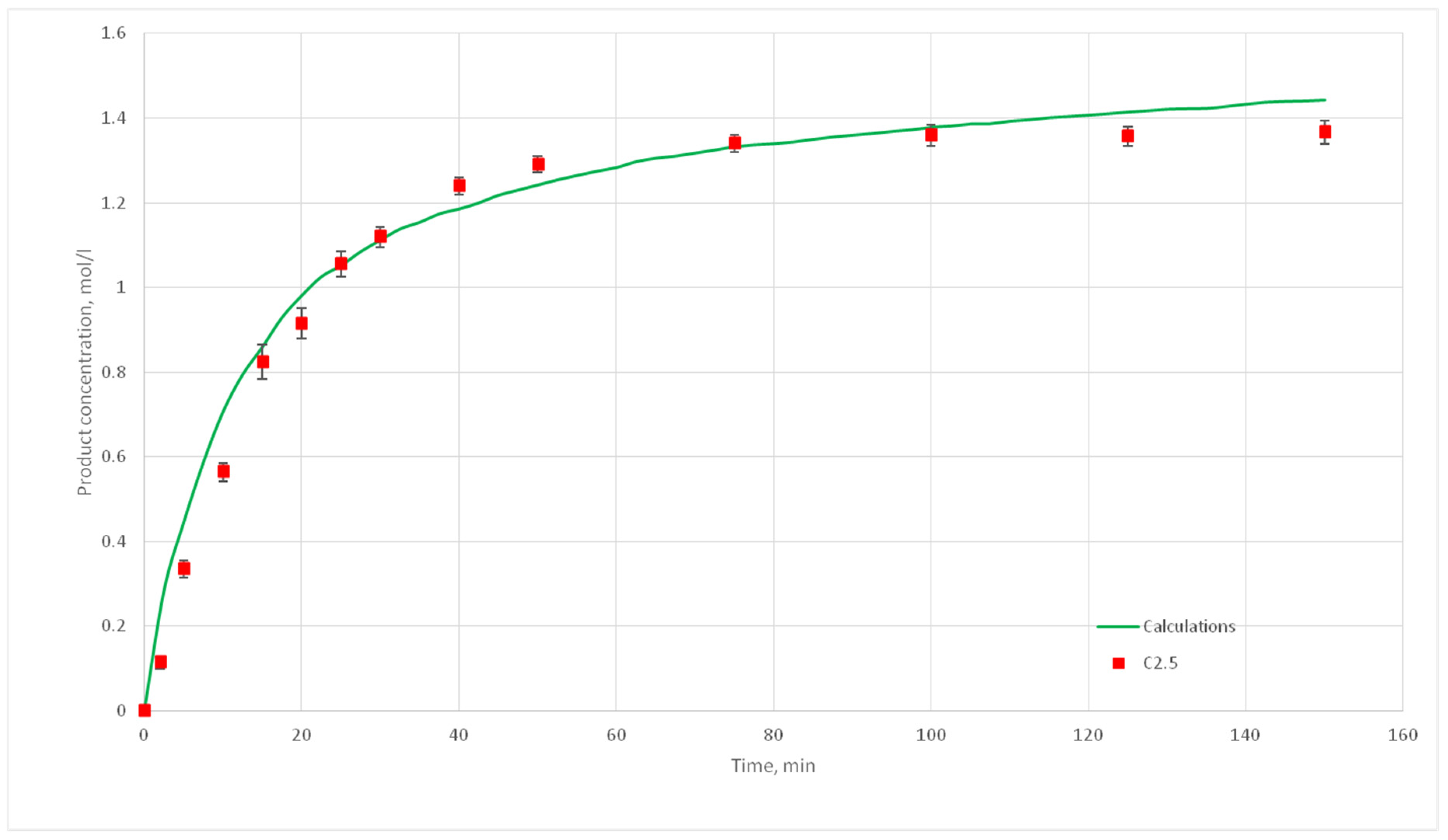
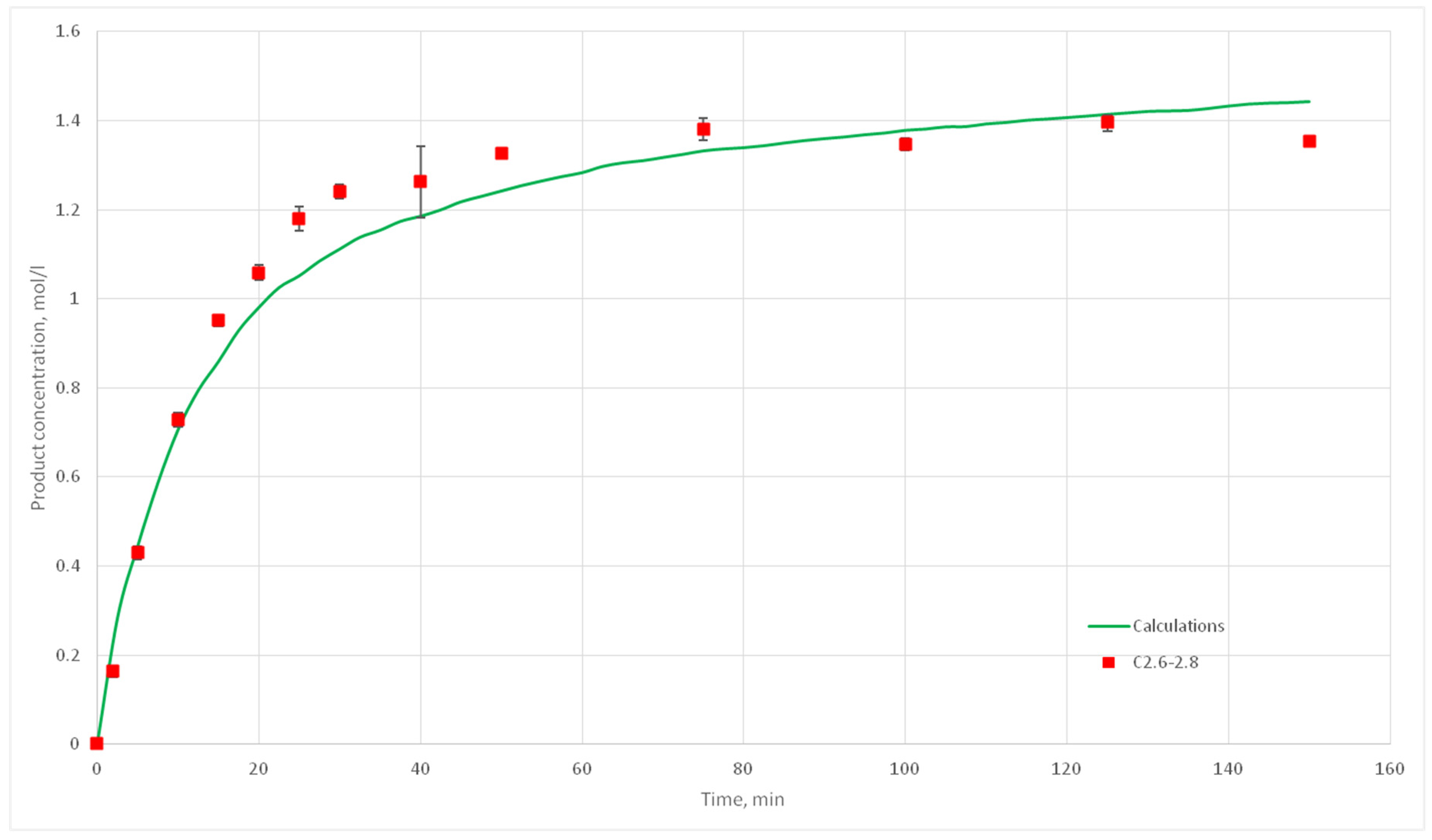
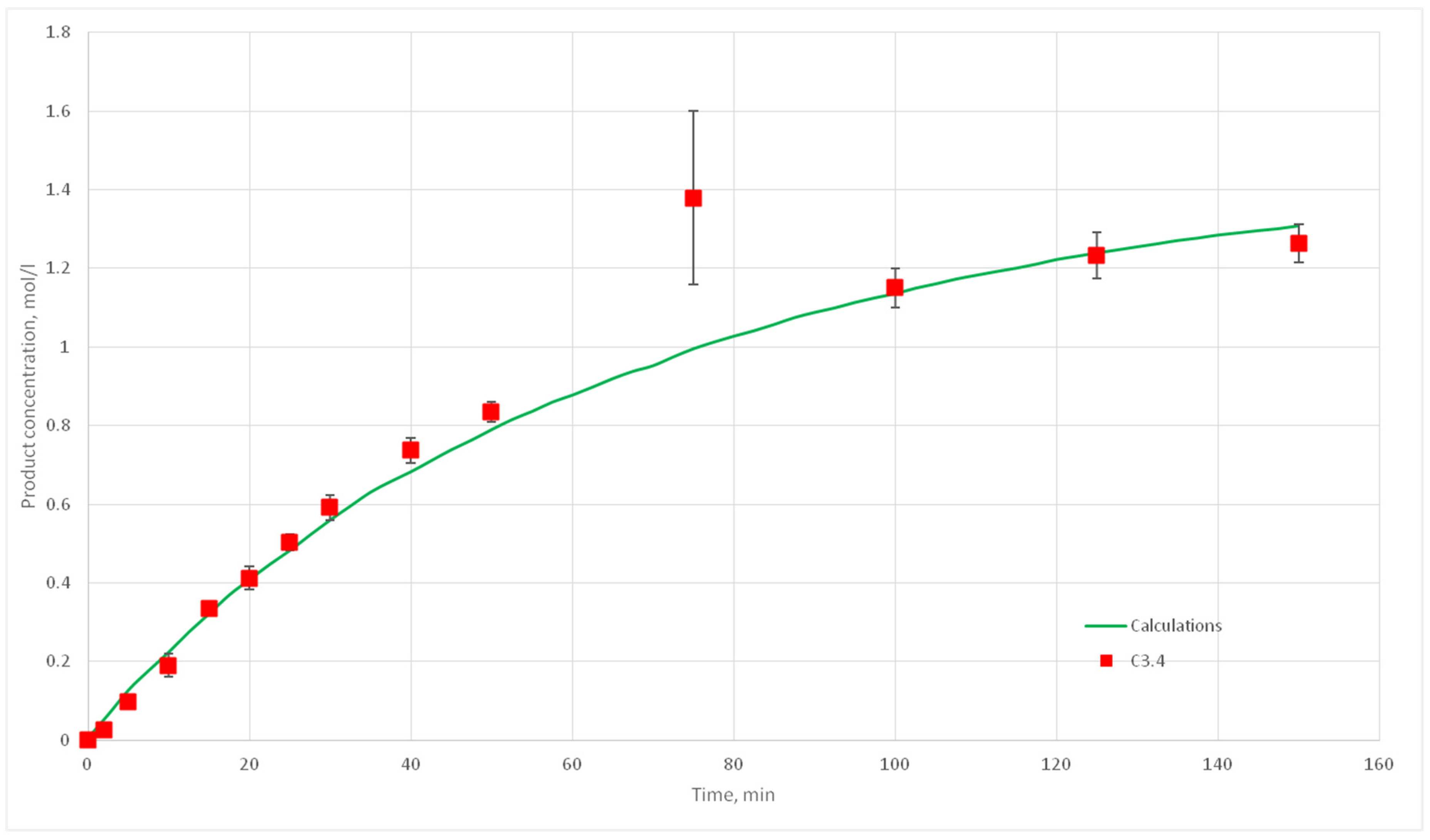
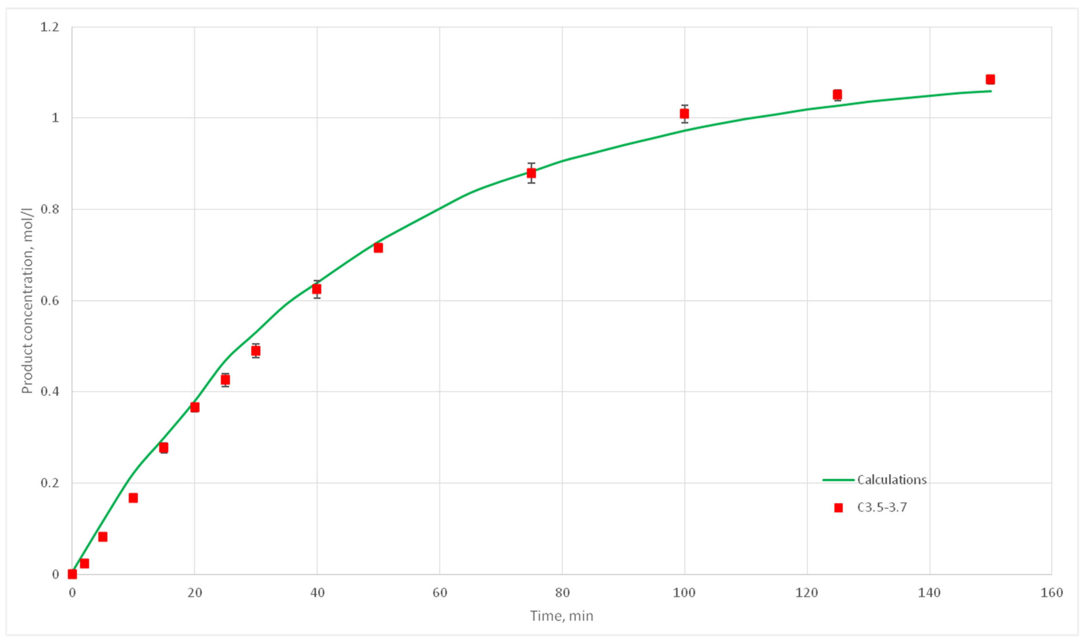
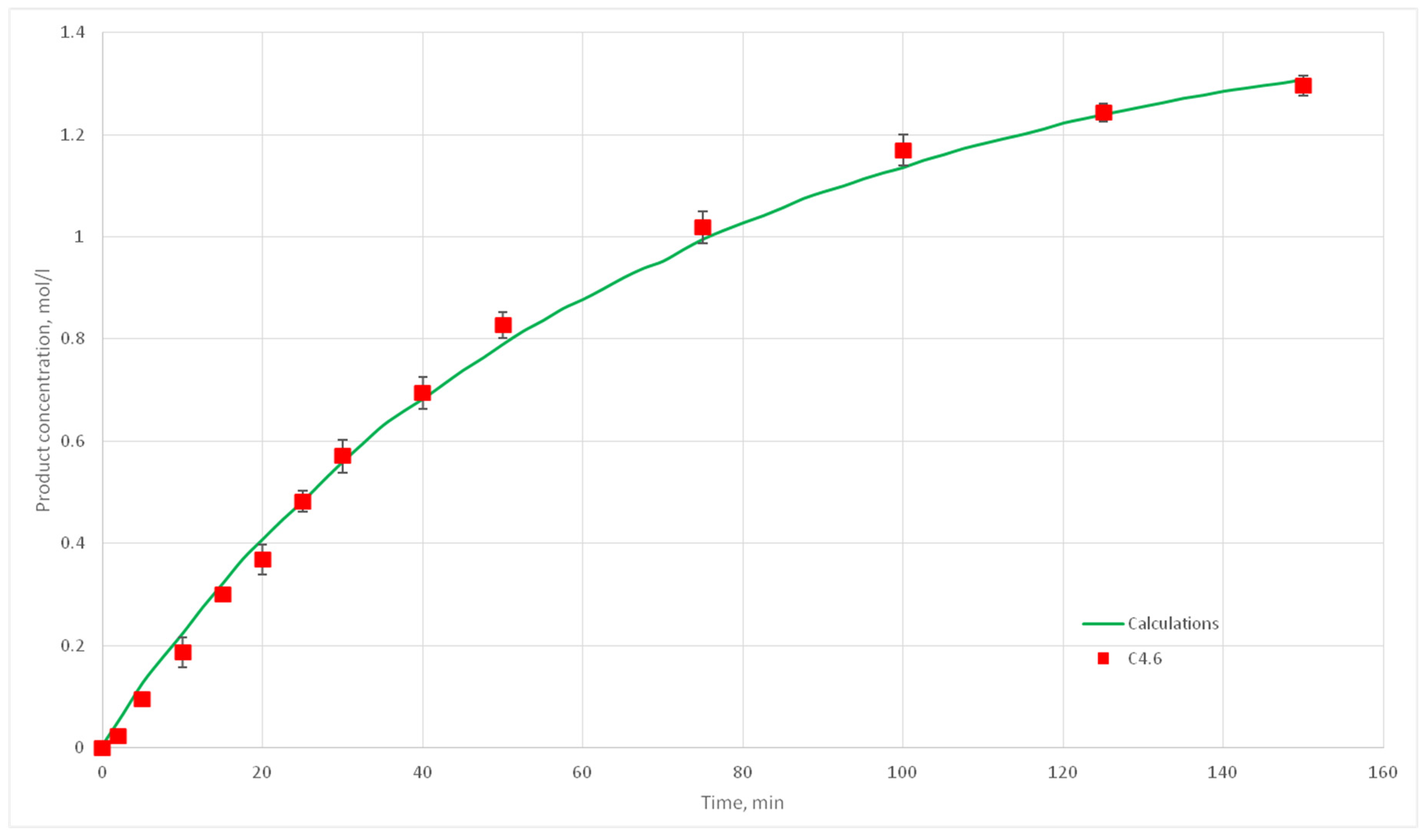
Eight computational experiments were carried out, resulting in kinetic curves obtained, corresponding to experiments C 2.1, 2.2, 2.3, 2.5, 2.6, 2.7, 2.8, 3.1, 3.2, 3.3, 3.4, 3.5, 3.6, 3.7, 4.6, 4.7, 4.8, and 4.9. Conditions for these experiments are shown in

Table 4. Experimental Conditions.

Experiments Series	Catalyst Concentration, g per Aniline Layer kg	Temperature, °C	Aniline: Formaldehyde Ratio	Stirrer Speed, rpm
C 2.1, 2.2, 2.3	40	110	5	500
C 2.5	120	110	5	500
C 2.6, 2.7, 2,8	160	110	5	500
C 3.1, 3.2, 3.3	40	110	4	500
C 3.4	40	110	5	500
C 3.5, 3.6, 3.7	40	110	6	500
C 4.6	40	110	5	500
C 4.7, 4.8, 4.9	40	130	5	500

. For each experiment three kinetic curves were obtained. So, for experiments C2.1–2.3, C2.6–2.8, C3.1–3.3, C3.5–3.7, and C4.7–4.9, nine kinetic curves were obtained.

Figure 18, Figure 19, Figure 20, Figure 21, Figure 22, Figure 23, Figure 24 and Figure 25 show a comparison of the calculated and experimental curves of the experimental data.

The deviation of the calculated curves from the experimental curves does not exceed 18%. Thus, it can be concluded, that the developed cellular automata model can be used to model the process of catalytic reactions involving aniline and formaldehyde and to predict the kinetic reaction curves.

4. Conclusions

In this work, the reactions of obtaining MDA in the presence of a catalyst were investigated. Kinetic curves were obtained under various conditions: aniline:formaldehyde:catalyst ratios, stirrer speed, and reaction temperature.

A cellular automata model was developed to predict the kinetic curves of the reactions studied. A total of 30 computational experiments were carried out to find the model parameters suitable for the reactions under study. Attained parameters made it possible to model the process of the studied catalytic reactions and predict the kinetic curves of these reactions with sufficient accuracy.

A total of eight computational experiments were carried out to predict the kinetic curves of the studied reactions. The obtained calculated curves deviated from the experimental ones by not more than 18%. Thus, the developed model of catalytic reactions allows the kinetic curves of the MDA production process to be predicted. In the future, the proposed CA model will be used together with the previously suggested CFD model. For this, the calculated CA model kinetic curves will be used to determine an additional mass source in continuity equations for the corresponding species. Furthermore, the local concentration of species from the CFD model will be used as a boundary condition for the CA model. This approach will allow, on the one hand, to accurately determine the kinetics of chemical reactions on a catalyst grain, taking into account its structural features, and on the other hand, to take into account the influence of hydrodynamics, convective mass transfer within the framework of arbitrary geometry and different parameters of the entire process. This will allow for the implementation of complex multiscale modeling of a flow catalytic reactor from the molecule level to the level of the entire apparatus. The suggested model will reduce the number of necessary experiments in the study of catalytic processes, partially replacing full-scale experiments with computational ones.