Combined Heat and Power Dynamic Economic Emissions Dispatch with Valve Point Effects and Incentive Based Demand Response Programs

Abstract

In this paper, the Combined Heat and Power Dynamic Economic Emissions Dispatch (CHPDEED) problem formulation is considered. This problem is a complicated nonlinear mathematical formulation with multiple, conflicting objective functions. The aim of this mathematical problem is to obtain the optimal quantities of heat and power output for the committed generating units which includes power and heat only units. Heat and load demand are expected to be satisfied throughout the total dispatch interval. In this paper, Valve Point effects are considered in the fuel cost function of the units which lead to a non-convex cost function. Furthermore, an Incentive Based Demand Response Program formulation is also simultaneously considered with the CHPDEED problem further complicating the mathematical problem. The decision variables are thus the optimal power and heat output of the generating units and the optimal power curbed and monetary incentive for the participating demand response consumers. The resulting mathematical formulations are tested on four practical scenarios depicting different system operating conditions and obtained results show the efficacy of the developed mathematical optimization model. Obtained results indicate that, when the Incentive-Based Demand Response (IBDR) program’s operational hours is unrestricted with a residential load profile, the energy curtailed is highest (2680 MWh), the energy produced by the generators is lowest (38,008.53 MWh), power losses are lowest (840.5291 MW) and both fuel costs and emissions are lowest.

1. Introduction

Combined Heat and Power (CHP) generating units also known as co-generation units produce electric power and heat simultaneously. The production of these two outputs as opposed to only power production significantly increases the efficiency of CHP units. Therefore, whilst conventional generation units have an efficiency of around 60% [1], CHP units have efficiency of around 90% [1]. An added advantage of CHP units over conventional units is that CHP units also yield lower emissions by about 13–18% [1]. The Combined Heat and Power Dynamic Economic Dispatch (CHPDED) problem seeks to minimize the fuel costs of committed units by determining their optimal power and heat output whilst also ensuring that both heat and power demand are satisfied during the whole scheduling interval [2]. This mathematical problem is constrained by practical mathematical constraints like ramp rate constraints, power balance constraint, generating units constraints, etc. Without the addition of ramp rate constraints, the CHPDED problem is simply referred to as the Combined Heat and Power Economic Dispatch (CHPED) [2]. The dynamic addition is due to the consideration of generator ramp rates which essentially sets a limit on heat and output power over consecutive time intervals in order to maintain the generator’s useful life. When factoring emissions into the CHPDED problem, there are three approaches to the resultant problem.

The first approach is to minimize both fuel costs and emissions whilst ensuring that power and heat demands are met. This approach is termed Combined Heat and Power Dynamic Economic Emission Dispatch (CHPDEED). The second approach involves the minimization of only fuel costs and defining a constraint which limits the amount of allowable emissions. This approach is termed the Combined Heat and Power Emission Constrained Dynamic Economic Dispatch (CHPECDED). The third approach is termed Combined Heat and Power Pure Dynamic Emission Dispatch (CHPPDED) concerned with the minimization of only emissions whilst ensuring that power and heat demands are met. In this work, the focus is on the CHPDEED problem which is a multi-objective optimization problem with two conflicting objective functions (minimization of fuel costs and harmful emissions). The multi objective function is converted to a single objective function by assigning weights to both objectives which allows for the determination of a trade-off between fuel costs and emissions.

In essence, the CHPDEED problem determines the committed units power and heat outputs whilst minimizing the fuel costs and emissions and respecting system constraints [1,2]. There are two main research focus areas in the CHPED/CHPDED/CHPECDED and CHPDEED research fields. The first is concerned with the development and application of novel solution methodologies and approaches. These solution methodologies cover both classical optimization algorithms and heuristic algorithms. Examples include [3] where the real coded genetic algorithm with improved Muhlenbein mutation is deployed to solve the CHPED problem. The solution algorithm is tested on sample case studies and returns feasible solutions. In Reference [2], differential evolution and sequential quadratic programming is deployed in solving the CHPDED problem and in [1] the same solution methodology is used to solve the CHPDED, CHPDEED, and CHPPDED. Another example is [4] where the utilization of integrated civilized swarm optimization and Powell’s pattern search method is used for the CHPED. Other examples include [5] and [6] where a “whale optimization method” is deployed to solve the CPHED problem. Other algorithms (solution methodologies) include the squirrel search algorithm [7], Kho–Kho optimization Algorithm [8], indicator and crowding distance-based evolutionary algorithm [9], cuckoo search algorithm [10,11], effective cuckoo search algorithm [12], exchange market algorithm [13], gravitational search algorithm [14], group search optimization algorithm [15], and modified group search optimizer [16]. A comprehensive review article on research works utilizing heuristic methods in solving the CHPDEED mathematical works is given in [17]. These heuristic solution algorithms are widely reported in literature and it is difficult to objectively report on the superiority of one algorithm over the other. In the final analysis, the choice of the heuristic solution algorithm is due to the bias of the researcher.

The second research focus area in the CHPED/CHPDED/CHPECDED and CHPDEED field deals with the incorporation of related power system sources or tasks when solving the mathematical optimization problem. In Reference [18], unit commitment which involves the determination of the ON/OFF status of generator units is performed together with economic dispatch for CHP units. In another work [19], dispatch is performed for a power system in China consisting of CHP units and wind turbines. Reference [20] performs dispatch for a CHP system including wind turbines and storage systems for both thermal and electrical energy. In [21], economic dispatch was performed for a micogrid consisting of CHP units, wind turbines, photovoltaic (PV) cells, battery storage, and gas fired boilers. Another work is [22] where a stochastic CHPED is performed for a system consisting of CHP units, wind turbines, and PV units. Chance constrained programming is utilized in solving the resultant model. In [23], the CHPDED problem is solved this time incorporating spinning reserve requirements and the resultant model is solved using an enhanced firefly algorithm.

The CHPDED problem has in recent times also been solved whilst incorporating demand response programs. Demand response programs are motivated primarily by the drive to curtail energy consumption on the demand side as opposed to increasing power generation on the supply side with its resultant financial implications [24,25,26]. Combining CHP and demand response programs is viewed as a cost effective way of maintaining today’s power system as CHP’s on the supply side have higher efficiency and lower emissions whilst demand response programs on the demand side introduce optimality and curtail consumer energy consumption. Hitherto, demand response programs have been incorporated into the economic dispatch of thermal units [25,26,27] and renewable energy systems [28]. However, only a few works focus on the joint optimization of CHP’s and demand response programs with CHP’s at the supply spectrum of the grid whilst demand response programs are at the demand spectrum of the grid. In Reference [29], a demand response scheme is integrated into a micro CHP system. A Model Predictive Control (MPC) solution methodology is utilized as the control algorithm and results indicate that the incorporation of demand response reduces cost about 1–14%. Reference [30] details a CHP system with demand response programs at the consumer side under a simulated energy hub. A comparison of various demand response schemes is provided and obtained results indicate that the incorporation of demand response programs reduce operation cots in the energy hub. In [31], the hourly scheduling of CHP units with demand response and storage facilities (energy and heat) is detailed. The case studies investigated from the paper shows that the implementation of demand response programs leads to cost reduction and improvement of grid reliability.

Recent works include [32] where a price based demand response program was formulated for combined heat and power consumers and [33] where a robust optimization framework was deployed for price based demand response programs integrated within a combined heat and power setup. An analysis of these prior works show that there is no integration of incentive based DR (IBDR) and CHP systems. Although it has been shown that incentive based demand response programs and CHP systems have the potential to be beneficial to utilities [34], practical investigations of this integration are lacking. This work therefore proposes a practical scheme for the optimal economic dispatch of CHP units with an incentive based demand response (IBDR) program. The resultant CHPDEED-IBDR problem has a non-smooth and non-convex objective function and provides an economic incentive for load curtailment in times of power system stress. The provided incentive is structured in such a way that it is greater than the curtailment cost and also factors in budgetary constraints amongst other practical constraints. Incorporating customer curtailment cost and ensuring that the incentive given is commensurate with the customer participation level and amount of curtailed power is referred to as “incentive compatibility”.

Most CHP units have an intertwined relationship between heat and power generation, thereby adding a significant degree of complexity to the problem. Thus, we ensure that the curtailment of electrical power doesn’t compromise the satisfaction of heat demand. Moreover, valve point effects and power losses are factored into the model. The developed multi-objective model with three objective models is converted into a single objective function with the use of a weighting method and the accuracy of the developed model is shown on four case studies with a high degree of success. The remainder of this article is thus given: The mathematical models for the CHPDEED-IBDR problem formulation is detailed in Section 2. Section 3 presents the methodology utilized for numerical simulations with Section 4 detailing results obtained via the simulations. Section 5 concludes the paper.

2. Combined Heat and Power Dynamic Economic Emission Dispatch Model

The CHPDEED mathematical model is made up of three distinct types of generators. They include: conventional thermal units (TU), CHP units, and heat-only units (H). Conventional thermal units and CHP units produce electric power whilst heat only units and CHP units produce heat. The CHPDEED mathematical problem has its objective as the minimization of the fuel costs and emissions of all units whilst satisfying the power and heat demand over the scheduling horizon under practical system constraints.

The individual fuel cost and emissions objective functions of all three types of generating units (thermal, CHP and heat) are detailed.

2.1. Thermal Units

The most common fuel function for thermal units is the quadratic representation [25,26,27]. A more accurate representation is one that incorporates valve point effects [1,2] given as:

$$C_i\left(P_{i,t}^{TU}\right)=a_i+b_i{P}_{i,t}^{TU}+c_i{\left(P_{i,t}^{TU}\right)}^2+e_{i}sin\left(f_i(P_{i,min}^{TU}-P_{i,t}^{TU})\right),$$

(1)

where

• $a_i$, $b_i$ and $c_i$ are the positive fuel cost coefficients of generator i respectively;
• $e_i$ and $f_i$ are the fuel cost coefficients representing valve point effects of generator i, respectively;
• $P_{i,t}^{TU}$ represents the power generated from thermal unit i at time t;
• $P_{i,min}^{TU}$ represents the minimum capacity of thermal unit i;
• $C_i\left(P_{i,t}^{TU}\right)$ represents the fuel cost of producing $P_{i,t}^{TU}$.

The emissions of thermal units are given by:

$$E_i^{TU}\left(P_{i,t}^{TU}\right)={\alpha }_i+{\beta }_i{P}_{i,t}^{TU}+{\gamma }_i{\left(P_{i,t}^{TU}\right)}^2+{\eta }_{i}exp\left({\delta }_i{P}_{i,t}^{TU}\right),$$

(2)

This emission mathematical function is a combined quadratic and exponential representation of the thermal units power output. ${\alpha }_i$, ${\beta }_i$, ${\gamma }_i$, ${\eta }_i$ and ${\delta }_i$ are the emission function coefficients of generator i and $E_i\left(P_{i,t}^{TU}\right)$ represents the total emissions to produce $P_{i,t}^{TU}$.

2.2. CHP Units

The CHP unit produces both power and heat. Thus, the fuel cost is a product of both outputs. This is usually represented as a convex cost function given as:

$$\begin{array}{c}{C}_k^{CHP}(P_{k,t}^{CHP},H_{k,t}^{CHP})=a_k+b_k{P}_{k,t}^{CHP}+c_k{\left(P_{k,t}^{CHP}\right)}^2+d_k{H}_{k,t}^{CHP}+e_k{\left(H_{k,t}^{CHP}\right)}^2\\ +f_k(P_{k,t}^{CHP},H_{k,t}^{CHP}),\end{array}$$

(3)

where

• $a_k$, $b_k$, $c_k$, $e_k$ and $f_k$ are the fuel cost coefficients of CHP generator l respectively;
• $C_k^{CHP}(P_{k,t}^{CHP},H_{k,t}^{CHP})$ is the fuel cost for CHP generator l to produce heat and power $(P_{k,t}^{CHP},H_{k,t}^{CHP})$.

The total CHP units emissions is solely a function of the power generated and is given as:

$$E_k^{CHP}\left(P_{k,t}^{CHP}\right)=({\alpha }_k+{\beta }_k)P_{k,t}^{CHP},$$

(4)

where ${\alpha }_k$ and ${\beta }_k$ are emission function coefficients.

2.3. Heat Units

These units produce only heat and the fuel cost function is depicted by:

$$C_l^H\left(H_{l,t}^H\right)=a_l+b_l{H}_{l,t}^H+c_l{\left(H_{l,t}^H\right)}^2,$$

(5)

where $a_l$, $b_l$ and $c_l$ are the positive fuel cost coefficients of generator l, respectively;

The emission function similarly is given by:

$$E_l^H\left(H_{l,t}^H\right)=({\alpha }_l+{\beta }_l)H_{l,t}^H,$$

(6)

where ${\alpha }_l$ and ${\beta }_l$ are the emissions coefficients of heat units l.

2.4. Objective Functions

The total fuel cost (for thermal, CHP and heat units) is given by:

$$C\left(PH\right)=\sum _{t=1}^T\left(\sum _{i=1}^I{C}_i^{TU}\left(P_{i,t}^{TU}\right)+\sum _{k=1}^K{C}_k^{CHP}(P_{k,t}^{CHP},H_{k,t}^{CHP})+\sum _{l=1}^L{C}_l^H\left(H_{l,t}^H\right)\right),$$

(7)

where T, I, K, and L are the total scheduling interval, total number of thermal units, total number of CHP units, and total number of heat units, respectively.

In a similar manner, the total emission function (for thermal, CHP and heat units) is given by:

$$E\left(PH\right)=\sum _{t=1}^T\left(\sum _{i=1}^I{E}_i^{TU}\left(P_{i,t}^{TU}\right)+\sum _{k=1}^K{E}_k^{CHP}\left(P_{k,t}^{CHP}\right)+\sum _{l=1}^L{E}_l^H\left(H_{l,t}^H\right)\right),$$

(8)

where T, I, K and L are the total scheduling interval, total number of thermal units, total number of CHP units, and total number of heat units, respectively.

2.5. Constraints

The constraints for the CHPDEED problem’s objective function (Equations (7) and (8)) are given below:

$$\sum _{i=1}^I{P}_{i,t}^{TU}+\sum _{k=1}^K{P}_{k,t}^{CHP}=D_t+los{s}_t,$$

(9)

$$\sum _{k=1}^K{H}_{k,t}^{CHP}+\sum _{l=1}^L{H}_{l,t}^H=H{D}_t+los{s}_t,$$

(10)

$$P_{i,min}^{TU}\le P_{i,t}^{TU}\le P_{i,max}^{TU},$$

(11)

$$P_{k,min}^{CHP}\left(H_{k,t}^{CHP}\right)\le P_{k,t}^{CHP}\le P_{k,max}^{CHP}\left(H_{k,t}^{CHP}\right),$$

(12)

$$H_{k,min}^{CHP}\left(P_{k,t}^{CHP}\right)\le H_{k,t}^{CHP}\le H_{k,max}^{CHP}\left(P_{k,t}^{CHP}\right),$$

(13)

$$H_{k,min}^H\le H_{k,t}^H\le H_{k,max}^H,$$

(14)

$$-D{R}_i^{TU}\le P_{i,t+1}^{TU}-P_{i,t}^{TU}\le U{R}_i^{TU},$$

(15)

$$-D{R}_k^{CHP}\le P_{k,t+1}^{CHP}-P_{k,t}^{CHP}\le U{R}_k^{CHP},$$

(16)

where

$$los{s}_t=\sum _{i=1}^I\sum _{z=1}^Z{P}_{i,t}{B}_{i,z}{P}_{z,t},$$

(17)

• $P_{i,t}^{TU}$ is the power generated from thermal generator i at time t;
• $P_{k,t}^{CHP}$ is the power generated from CHP generator k at time t;
• $H_{k,t}^{CHP}$ is the heat produced from CHP generator k at time t;
• $H_{l,t}^H$ is the heat produced from heat generator l at time t;
• $D_t$ is the total system power demand at time t;
• $H{D}_t$ is the total system heat demand at time t;
• $los{s}_t$ is the total system losses at time t;
• $P_{i,min}^{TU}$ and $P_{i,max}^{TU}$ are the minimum and maximum power capacity of thermal generator i respectively;
• $H_{l,min}^H$ and $H_{l,max}^H$ are the minimum and maximum heat capacities of generator l respectively;
• $P_{k,min}^{CHP}\left(H_{k,t}^{CHP}\right)$ and $P_{k,max}^{CHP}\left(H_{k,t}^{CHP}\right)$ are the minimum and maximum power capacities of CHP generator k, respectively. Both parameters are functions of the heat produced $\left(H_{k,t}^{CHP}\right)$.
• $H_{k,min}^{CHP}\left(P_{k,t}^{CHP}\right)$ and $H_{k,max}^{CHP}\left(P_{k,t}^{CHP}\right)$ are the minimum and maximum heat capacities of CHP generator k, respectively. Both parameters are functions of the power produced $\left(P_{k,t}^{CHP}\right)$.
• $D{R}_i^{TU}$ and $U{R}_i^{TU}$ are the maximum ramp down and up rates of thermal generator i, respectively;
• $D{R}_k^{CHP}$ and $U{R}_k^{CHP}$ are the maximum ramp down and up rates of CHP generator k, respectively;
• $B_{i,z}$ is the $iz$th element of the loss coefficient square matrix of size $I+L$;

Equations (9)–(16) represent the constraints of the mathematical model and their interpretation is given as:

• Constraint (9) is termed the “power balance constraint”. Its role is to compel the total output power from both thermal and CHP units at each scheduling interval to satisfy the load demand and transmission line losses. Transmission line losses are determined by the B-coefficient method [1,2] and is represented mathematically in (17). $B_{i,z}$ is the $iz$th element of the loss coefficient square matrix B of size $I+L$. This method has been used in [25,26,27].
• Constraint (10) is termed the “heat balance constraint” and its role is to compel the heat output from both CHP and heat-only units to match heat demand.
• The third constraint is the thermal generation limits constraint (11). It compels the output power from thermal generators to not exceed allowed limits.
• The fourth constraint (12) limits power produced from CHP units within allowable units.
• The fifth constraint (13) limits heat produced from CHP units within allowable limits.
• Constraint (14) ensures that the heat produced from heat only units are within allowable limits.
• Constraint (15) is the “generator ramp rate limits constraint” for thermal generators and compels the thermal generators output power for consecutive scheduling intervals to be within allowable ramp rate limits.
• Constraint (16) is termed “generator ramp rate limits constraint” for CHP generators. Similar to constraint (15), it compels the output power for CHP units for consecutive scheduling intervals to be within allowable ramp rate limits.

The two objective functions (Equations (7) and (8)) can be concatenated into a single objective function via a weighting factor w. The resultant single objective function is still constrained by (9)–(17):

$$min\left[wC\left(PH\right)+(1-w)E\left(PH\right)\right].$$

(18)

where w and $(1-w)$ are weighting factors. The condition to be satisfied is [27,35]:

$$w+(1-w)=1.$$

(19)

Both weighting factors are non-negative and can be controlled by the modeler based on the preference given to objective functions. When the modeler seeks to minimize fuel costs alone, then $w=1$ (CHPDED). However, when the modeler wants to minimize emissions alone, then $w=0$ (CHPPDED). It is assumed for the purpose of this article that equal weights are given to both objective functions. Thus, $w=(1-w)=0.5$.

3. Incentive Based Demand Response Model

If we assume that an electric consumer/customer of type $\theta$ is willing to curb x MW of power. The customer benefit function can therefore be represented, thus:

$$V_1(\theta ,x,y)=y-c(\theta ,x),$$

(20)

where y is the incentive (monetary value) the customer is given. Customer participation is only guaranteed if $V_1\ge 0$. In the same vein, the electric utility’s benefit function is given as:

$$V_2(\theta ,\lambda )=\lambda x-y.$$

(21)

$\lambda$ is the Locational Marginal Price (LMP) or “value of power interruptibility” [26,27] and is calculated from Optimal Power Flow (OPF) routines. We can thus define the utility’s benefit function (benefit maximization) as:

$$\underset{x,y}{max}[\lambda x-y],$$

(22)

where

• $\theta$ is the “customer type”, normalized in $[0,1]$.
• x is the amount of power curbed by electric consumer/customer.
• $c(\theta ,x)$ is the cost of reducing x MW by customer of type $\theta$.
• $\lambda$ is the “value of power interruptibility” or LMP.

Customer Cost Function

$c(\theta ,x)$ is the cost to electric consumer/customer of type $\theta$ who curbs x MW of electric power. A quadratic customer cost function is assumed represented thus:

$$c(\theta ,x)=K_1{x}^2+K_{2}x-K_{2}x\theta ,$$

(23)

where $K_1$ and $K_2$ are customer cost co-efficients. $\theta$ is the customer type [26,27] and classifies electric consumers/customers based on the amount of power they are curbing. $\theta$ is normalized in the interval $0\le \theta \le 1$, thus $\theta =1$ is the keenest consumer/customer and $\theta =0$ is the least keen. The customer cost function satisfies the following conditions:

• Quadratic function: $c(\theta ,x)=K_1{x}^2+K_{2}x-K_{2}x\theta .$
• $K_{2}x\theta$ term sorts customers by way of $\theta$.
• Marginal cost decreases with an increase in $\theta$: Customer ($\theta =1$), who is the keenest customer, will therefore have the lowest marginal cost and the largest marginal benefit. Customer ($\theta =0$), who is the least keen customer, will have the largest marginal cost and lowest marginal benefit:
• $\partial c/\partial x=2K_{1}x+K_2-K_2\theta$.
• Non-negative marginal cost.
• The marginal cost function is an increasing convex cost function.
• When no power is curtailed, then the customer cost should be zero ($c(\theta ,0)=0$).

If $y_j$ is the incentive for customer j, customer benefit [26,27] is:

$$u_j=y_j-(K_1{x}^2+K_{2}x-K_{2}x\theta ),forj=1,\dots ,J,$$

(24)

The utility benefit is given as:

$$u_o=\sum _{j=1}^J{\lambda }_j{x}_j-y_j.$$

(25)

The incentive Based DR program seeks to therefore maximize the utility benefit:

$$ma{x}_{x,y}\sum _{j=1}^J[{\lambda }_j{x}_j-y_j],$$

(26)

s.t.

$$y_j-(K_1{x}_j^2+K_2{x}_j-K_2{x}_j{\theta }_j)\ge 0,forj=1,\dots ,J,$$

(27)

$$\begin{array}{c}{y}_j-(K_1{x}_j^2+K_2{x}_j-K_2{x}_j{\theta }_j)\ge y_{j-1}-(K_1{x}_{j-1}^2+K_2{x}_{j-1}-K_2{x}_{j-1}{\theta }_{j-1}),\\ forj=2,\dots ,J,\end{array}.$$

(28)

• Constraint (27) is the “individual rationality constraint” and compels the customer benefit to be greater or at least zero.
• Constraint (28) is the “incentive compatibility constraint” and compels customers to be compensated commensurate to the load they curtail.

There are two variables: customer power curtailed (x MW) and the customer incentive ($ y). Furthermore, we expand the model over more than one scheduling interval and incorporate other practical considerations into the model. The resulting model is detailed thus:

$$ma{x}_{x,y}\sum _{t=1}^T\sum _{j=1}^J[{\lambda }_{j,t}{x}_{j,t}-y_{j,t}],$$

(29)

s.t.

$$\sum _{t=1}^T[y_{j,t}-(K_{1,j}{x}_{j,t}^2+K_{2,j}{x}_{j,t}-K_{2,t}{x}_{j,t}{\theta }_j)]\ge 0,forj=1,\dots ,J,$$

(30)

$$\begin{array}{c}\sum _{t=1}^T[y_{j,t}-(K_{1,j}{x}_{j,t}^2+K_{2,j}{x}_{j,t}-K_{2,t}{x}_{j,t}{\theta }_j)]\ge \\ \sum _{t=1}^T[y_{j-1,t}-(K_{1,j-1}{x}_{j-1,t}^2+K_{2,j-1}{x}_{j-1,t}-K_{2,j-1}{x}_{j-1,t}{\theta }_{j-1})],\\ forj=2,\dots ,J,\end{array}.$$

(31)

$$\sum _{t=1}^T\sum _{j=1}^J{y}_{j,t}\le UB,$$

(32)

$$\sum _{t=1}^T{x}_{j,t}\le C{M}_j,$$

(33)

where $UB$ is the utility’s total budget and $C{M}_j$ is the maximum amount of power customer j is willing to curb in a day;

• The first constraint (30) makes sure that each customer’s daily incentive is greater than their interruption cost.
• The second constraint (31) makes sure that each customer’s benefit is commensurate with their power curtailment.
• The third constraint (32) compels the total monetary value of incentives paid by the electric utility to be within its budgeted amount.
• The fourth constraint (33) compels the total daily power curbed by each customer to be within its allowable daily limits.

4. Combined Heat and Power Dynamic Economic Emissions Dispatch with Incentive Based Demand Response Model

The final combined mathematical model can be represented as follows:

$$\begin{array}{c}min{w}_1\left[\sum _{t=1}^T\sum _{i=1}^I{C}_i^{TU}\left(P_{i,t}^{TU}\right)+\sum _{k=1}^K{C}_k^{CHP}(P_{k,t}^{CHP},H_{k,t}^{CHP})+\sum _{l=1}^L{C}_l^H\left(H_{l,t}^H\right)\right]\\ +w_2\left[\sum _{t=1}^T\sum _{i=1}^I{E}_i^{TU}\left(P_{i,t}^{TU}\right)+\sum _{k=1}^K{E}_k^{CHP}\left(P_{k,t}^{CHP}\right)+\sum _{l=1}^L{E}_l^H\left(H_{l,t}^H\right)\right]\\ +w_3\left[\sum _{t=1}^T\sum _{j=1}^J\left[y_{j,t}-{\lambda }_{j,t}{x}_{j,t}\right]\right]\end{array}$$

(34)

subject to

$$\sum _{i=1}^I{P}_{i,t}^{TU}+\sum _{k=1}^K{P}_{k,t}^{CHP}=D_t+los{s}_t,$$

(35)

$$\sum _{k=1}^K{H}_{k,t}^{CHP}+\sum _{l=1}^L{H}_{l,t}^H=H{D}_t+los{s}_t,$$

(36)

$$P_{i,min}^{TU}\le P_{i,t}^{TU}\le P_{i,max}^{TU},$$

(37)

$$P_{k,min}^{CHP}\left(H_{k,t}^{CHP}\right)\le P_{k,t}^{CHP}\le P_{k,max}^{CHP}\left(H_{k,t}^{CHP}\right),$$

(38)

$$H_{k,min}^{CHP}\left(P_{k,t}^{CHP}\right)\le H_{k,t}^{CHP}\le H_{k,max}^{CHP}\left(P_{k,t}^{CHP}\right),$$

(39)

$$H_{k,min}^H\le H_{k,t}^H\le H_{k,max}^H,$$

(40)

$$-D{R}_i^{TU}\le P_{i,t+1}^{TU}-P_{i,t}^{TU}\le U{R}_i^{TU},$$

(41)

$$-D{R}_k^{CHP}\le P_{k,t+1}^{CHP}-P_{k,t}^{CHP}\le U{R}_k^{CHP},$$

(42)

$$\sum _{t=1}^T[y_{j,t}-(K_{1,j}{x}_{j,t}^2+K_{2,j}{x}_{j,t}-K_{2,t}{x}_{j,t}{\theta }_j)]\ge 0,forj=1,\dots ,J,$$

(43)

$$\begin{array}{c}\sum _{t=1}^T[y_{j,t}-(K_{1,j}{x}_{j,t}^2+K_{2,j}{x}_{j,t}-K_{2,t}{x}_{j,t}{\theta }_j)]\ge \\ \sum _{t=1}^T[y_{j-1,t}-(K_{1,j-1}{x}_{j-1,t}^2+K_{2,j-1}{x}_{j-1,t}-K_{2,j-1}{x}_{j-1,t}{\theta }_{j-1})],\\ forj=2,\dots ,J,\end{array}.$$

(44)

$$\sum _{t=1}^T\sum _{j=1}^J{y}_{j,t}\le UB,$$

(45)

$$\sum _{t=1}^T{x}_{j,t}\le C{M}_j,$$

(46)

$$w_1+w_2+w_3=1.$$

(47)

5. Numerical Simulations, Results, and Discussion

5.1. Numerical Simulations

In order to investigate the efficacy of our proposed mathematical formulations (CHPDEED-IBDR), four different cases are used. The cases differ based on their load profile and are detailed as:

• CHPDEED-IBDR with residential load.
• CHPDEED-IBDR with residential load with restrictions on DR operating hours.
• CHPDEED-IBDR with commercial load.
• CHPDEED-IBDR with commercial load with restrictions on DR operating hours.

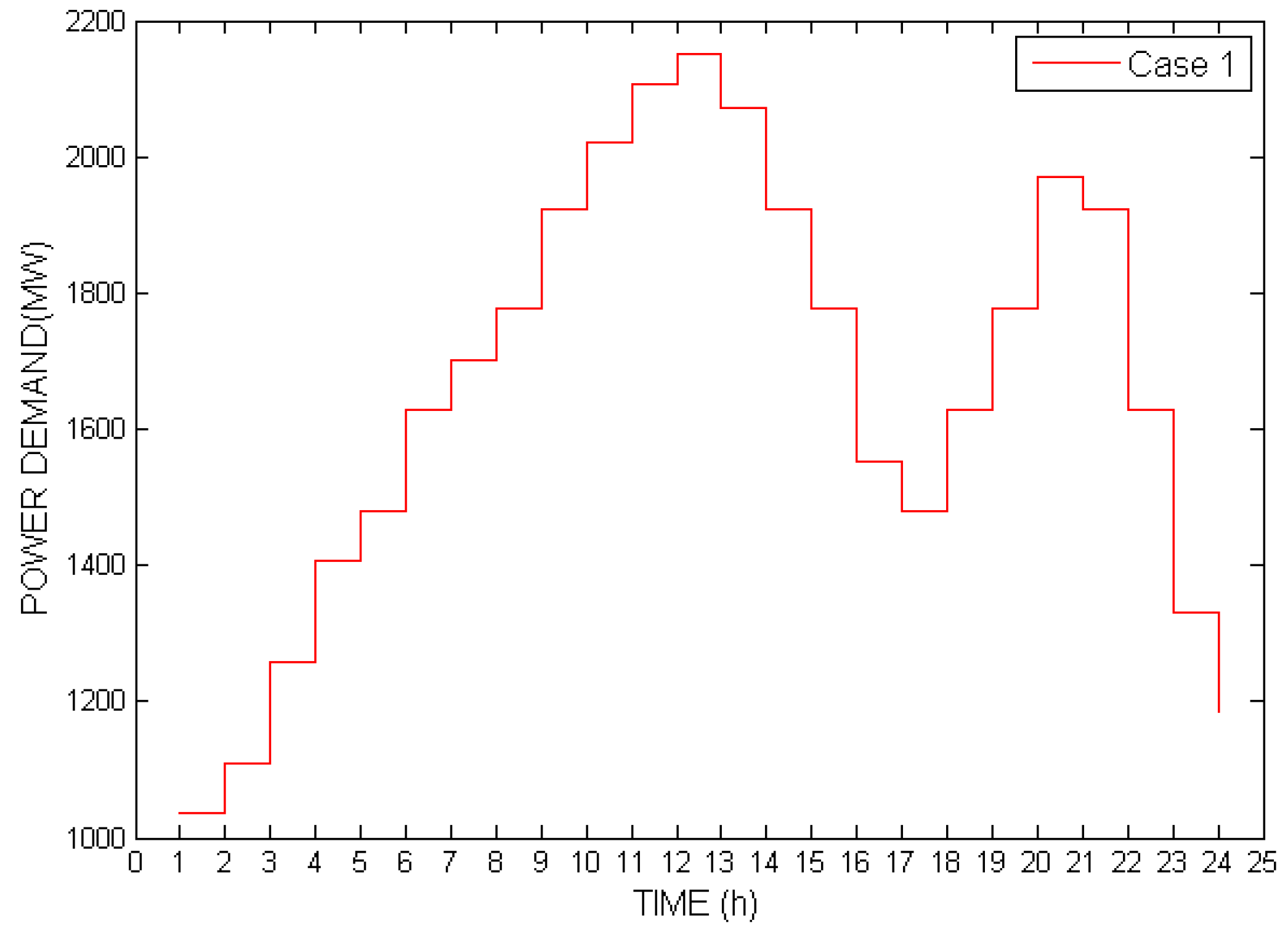
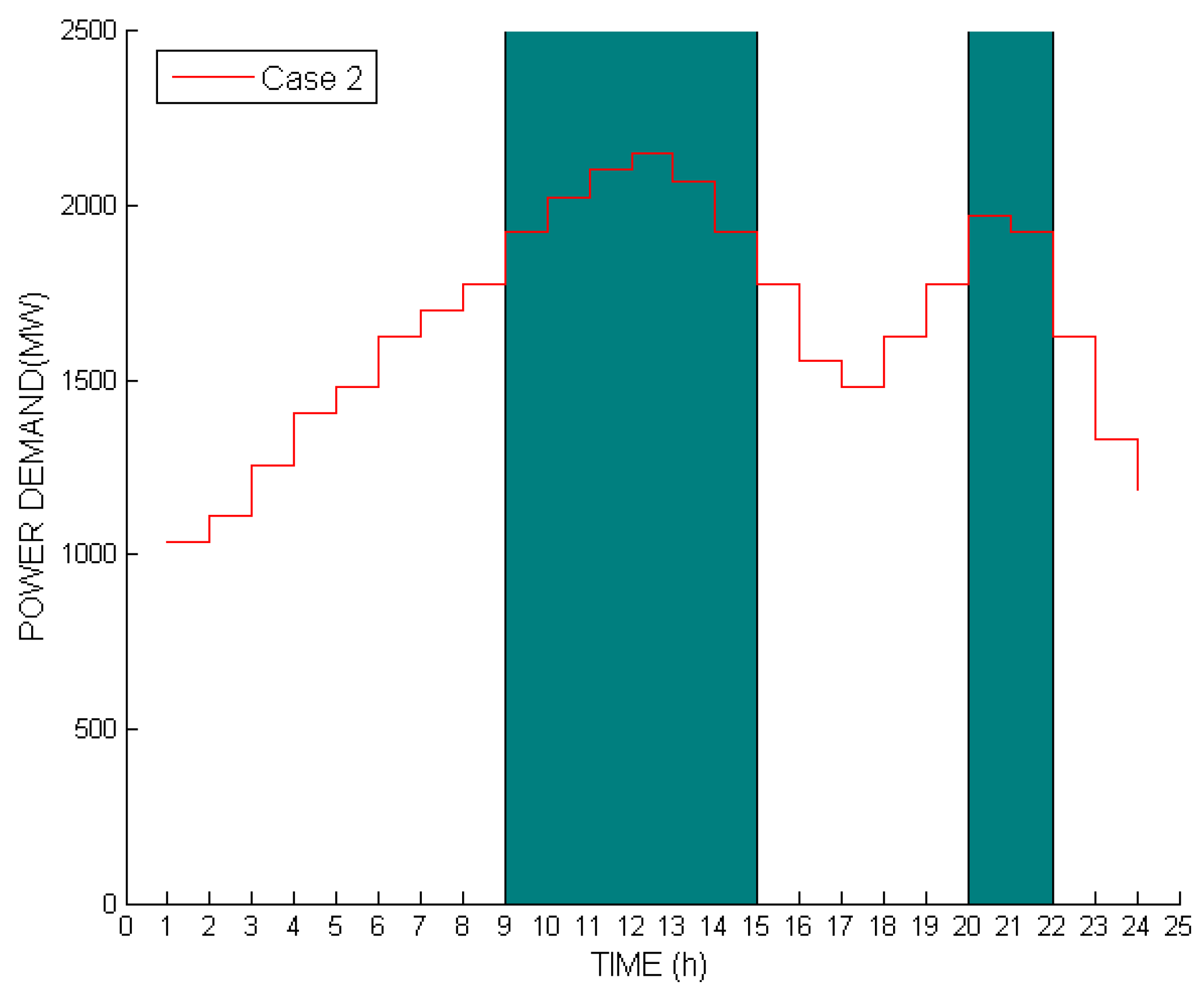
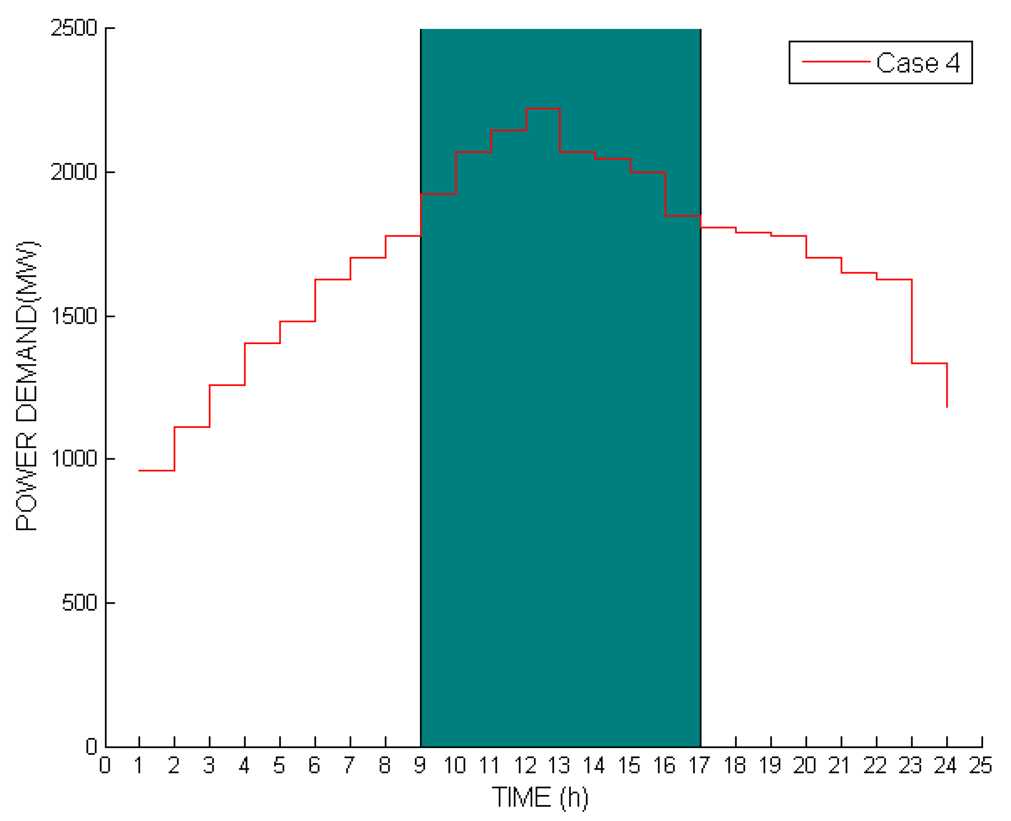
The load profile of Cases 1–4 are given in Figure 1, Figure 2, Figure 3 and Figure 4, respectively. Figure 2 and Figure 4 correspond to Case 2 and Case 4 with the colored areas depicting the allowed IBDR operating hours.

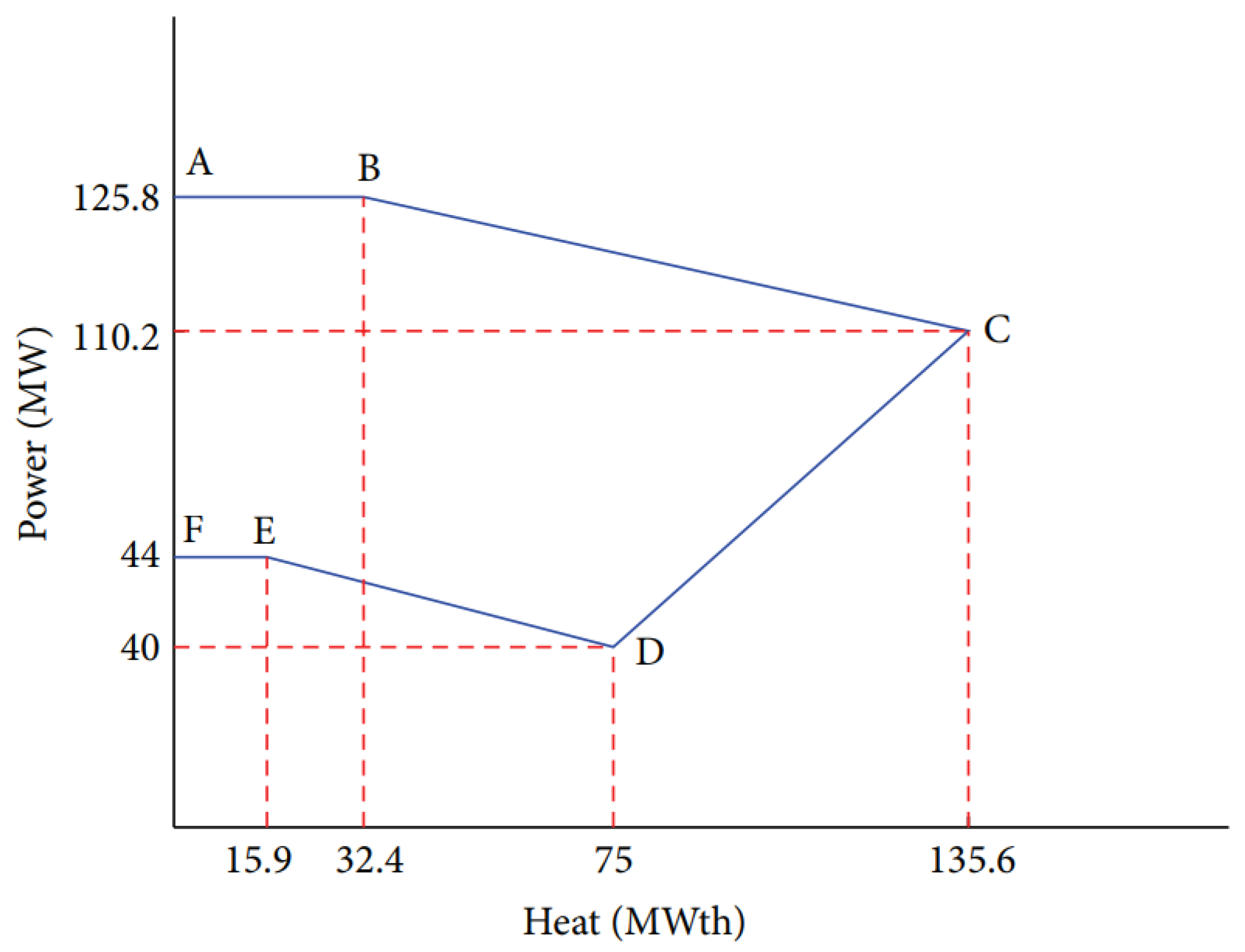
For all case studies, the eleven unit system consisting of (eight conventional units, two CHP units, and one heat-only unit) is utilized. The data for the conventional, CHP, and heat units are given in

Table 1. Data of thermal units.

Thermal Units	${\mathit{a}}_{\mathit{i}}$	${\mathit{b}}_{\mathit{i}}$	${\mathit{c}}_{\mathit{i}}$	${\mathit{e}}_{\mathit{i}}$	${\mathit{f}}_{\mathit{i}}$	${\mathit{\alpha }}_{\mathit{i}}$	${\mathit{\beta }}_{\mathit{i}}$	${\mathit{\gamma }}_{\mathit{i}}$	${\mathit{\eta }}_{\mathit{i}}$	${\mathit{\delta }}_{\mathit{i}}$	${\mathit{P}}_{\mathit{i},\mathit{min}}^{\mathit{TU}}$	${\mathit{P}}_{\mathit{i},\mathit{max}}^{\mathit{TU}}$	${\mathit{DR}}_{\mathit{i}}^{\mathit{TU}}={\mathit{UR}}_{\mathit{i}}^{\mathit{TU}}$
i = 1	786.7988	38.5397	0.1524	450	0.041	103.3908	2.4444	0.0312	0.5035	0.0207	150	470	80
i = 2	451.3251	46.1591	0.1058	600	0.036	103.3908	2.4444	0.0312	0.5035	0.0207	135	470	80
i = 3	1049.998	40.3965	0.028	320	0.028	300.391	4.0695	0.0509	0.4968	0.0202	73	340	80
i = 4	1243.531	38.3055	0.0354	260	0.052	300.391	4.0695	0.0509	0.4968	0.0202	60	300	50
i = 5	1356.659	38.2704	0.0179	310	0.048	320.0006	3.8132	0.0344	0.4972	0.02	57	160	50
i = 6	1450.705	36.5104	0.0121	300	0.086	330.0056	3.9023	0.0465	0.5163	0.0214	20	130	30
i = 7	1455.606	39.5804	0.109	270	0.098	350.0056	3.9524	0.0465	0.5475	0.0234	20	80	30
i = 8	1469.403	40.5407	0.1295	380	0.094	360.0012	3.9864	0.047	0.5475	0.0234	10	55	30

,

Table 2. Data of CHP Units.

CHP Units	${\mathit{a}}_{\mathit{k}}$	${\mathit{b}}_{\mathit{k}}$	${\mathit{c}}_{\mathit{k}}$	${\mathit{d}}_{\mathit{k}}$	${\mathit{e}}_{\mathit{k}}$	${\mathit{f}}_{\mathit{k}}$	${\mathit{\alpha }}_{\mathit{k}}$	${\mathit{\beta }}_{\mathit{k}}$	${\mathit{DR}}_{\mathit{k}}^{\mathit{CHP}}={\mathit{UR}}_{\mathit{k}}^{\mathit{CHP}}$ (MW/h)
k = 1	2650	14.5	0.0345	4.2	0.03	0.031	0.00015	0.00015	70
k = 2	1250	36	0.0435	0.6	0.027	0.011	0.00015	0.00015	50

and

Table 3. Data of heat only unit.

Heat Unit	${\mathit{a}}_{\mathit{l}}$	${\mathit{b}}_{\mathit{l}}$	${\mathit{c}}_{\mathit{l}}$	${\mathit{\alpha }}_{\mathit{l}}$	${\mathit{\beta }}_{\mathit{l}}$	${\mathit{H}}_{\mathit{l},\mathit{min}}^{\mathit{H}}$ (MW/h)	${\mathit{H}}_{\mathit{l},\mathit{max}}^{\mathit{H}}$ (MW/h)
l = 1	950	2.0109	0.038	0.0008	0.001	0	2695.2

, respectively, and is obtained from [1,2]. Feasible operating regions for the CHP units are given in Figure 5 and Figure 6, respectively. The power and heat demand are given in

Table 4. Heat demand and power demand.

Hour	Heat Demand (MWth)	Case 1 Demand (MW)	Case 3 Demand (MW)
1	390	1036	963
2	400	1110	1110
3	410	1258	1258
4	420	1406	1406
5	440	1480	1480
6	450	1628	1628
7	450	1702	1702
8	455	1776	1776
9	460	1924	1924
10	460	2022	2072
11	470	2106	2146
12	480	2150	2220
13	470	2072	2072
14	460	1924	2050
15	450	1776	2000
16	450	1554	1850
17	420	1480	1805
18	435	1628	1792
19	445	1776	1776
20	450	1972	1705
21	445	1924	1650
22	435	1628	1628
23	400	1332	1332
24	400	1184	1184

and the customer data are detailed in

Table 5. Customer cost function coefficients, customer type, and daily customer energy limit.

j	${\mathit{K}}_{1,\mathit{j}}$	${\mathit{K}}_{2,\mathit{j}}$	${\mathit{\theta }}_{\mathit{j}}$	${\mathit{CM}}_{\mathit{j}}$ (MW/h)
1	1.847	11.64	0	180
2	1.378	11.63	0.14	230
3	1.079	11.32	0.26	310
4	0.9124	11.5	0.37	390
5	0.8794	11.21	0.55	440
6	1.378	11.63	0.84	530
7	1.5231	11.5	1	600

. The transmission loss formula coefficients for the thermal only units and the CHP units are given by Equations (48) and (49), respectively. The customer data (values of power interruptibility (LMP) and customer parameters: $K_{1,j}$ and $K_{2,j}$) are obtained from [26,27]. The daily limit of interruptible energy ($C{M}_j$) is utilized by the ISO to determine customer keenness ${\theta }_j$. The ISO’s daily budget ($UB$) is given as $ 100,000. A key assumption made is that the heat demand is always satisfied and it is only the power demand that is curtailed via the demand response program. Cases 2 and 4 are cases when the DR programs have restricted operating hours. For Case 2, the IBDR program can only operate between 0900–1500 h and 2000–2200 h. Case 4 IBDR operation hours lies between 0900–1700 h. The Advanced Interactive Multidimensional Modeling System (AIMMS) via the CONOPT solver [36] is used to model and solve the developed optimization models.

$$B={10}^{-5}\times \left[\begin{array}{cccccccc}4.90& 1.40& 1.50& 1.50& 1.70& 1.70& 1.90& 2.00\\ 1.40& 4.50& 1.60& 1.60& 1.50& 1.50& 1.80& 1.80\\ 1.50& 1.60& 3.90& 1.00& 1.20& 1.40& 1.60& 1.60\\ 1.50& 1.60& 1.00& 4.00& 1.00& 1.10& 1.40& 1.50\\ 1.70& 1.50& 1.20& 1.00& 3.60& 1.30& 1.40& 1.50\\ 1.70& 1.50& 1.40& 1.10& 1.20& 3.80& 1.60& 1.80\\ 1.90& 1.80& 1.60& 1.40& 1.40& 1.60& 4.20& 1.90\\ 2.00& 1.80& 1.60& 1.50& 1.50& 1.80& 1.90& 4.40\end{array}\right]perMW$$

(48)

$$B={10}^{-5}\times \left[\begin{array}{cc}3.50& 1.30\\ 1.30& 4.00\end{array}\right]perMW$$

(49)

5.2. Results and Discussion

The multi-objective optimization problem has three objective functions and we assume that equal objectives were given to all three objectives. Thus, $w_1=w_2=w_3=0.333$. Figure 7, Figure 8, Figure 9 and Figure 10 give the initial load profiles and final load profiles after the IBDR program for cases 1, 2, 3, and 4, respectively. From the figures, it is obvious that the incorporation of the IBDR program leads to a reduction in the demand across all cases (commercial and industrial load profiles). The full results for all cases is given in

Table 6. Results for the case studies.

Parameters	Case 1	Case 2	Case 3	Case 4
Fuel Cost ($)	2,266,792	2,311,892	2,330,577	2,376,601
Emissions (lb)	458,955.4	475,320.5	478,319	494,630.5
Total Energy Generated (MWh)	38,008.53	38,712.67	38,732.62	39,439.46
Total Heat (MWth)	10,545	10,545	10,545	10,545
Total Losses (MW)	840.5291	871.2289	883.6219	914.9209
Total Incentive ($)	100,000	100,000	100,000	100,000
Total Energy Saved (MWh)	2680	2006.561	2680	2004.458
Cost of Energy ($/MWh)	62.27	62.30	62.75	62.79

. It shows the fuel cost ($), emissions (lb), total energy generated (MWh), total heat (MWth), total losses (MW), total incentive ($), and total energy saved/curtailed (MWh) for all cases over 24 h. In order to benchmark the CHPDEED-IBDR results, results from conventional CHPDEED using the data of Case 1 are also provided in the second column of Table 6.

For Case 1 and Case 3, when there is no restriction in IBDR operating hours (utilities might loathe requiring customers to restrict their demand for 24 h), the total energy generated by both the thermal units and CHP units over 24 h is 38,008.53 MWh and 38,732.62 MWh, respectively. Again, for both cases, the total energy saved or curtailed by the IBDR program is 2680 MWh. Both cases also have low power losses of 840.53 MW and 883.62 MW, respectively. Cases 2 and 4 are cases when the operational hours of the IBDR program are restricted to 0900–1500 h and 2000–2200 h (Case 2) and 0900–1700 (Case 4). To provide a fair comparison, the only difference between Cases 1 and 2 and Cases 3 and 4 is the IBDR operational hours. The utility budget is assumed constant in all cases at $100 000.

From the results obtained, Case 2 generates more energy than Case 1 (38,712.67 MWh to 38,008.53 MWh). In addition, Case 4 generates more energy than Case 3 (39,439.46 MWh to 38,732.62 MWh). This is expected and is due to the fact that the energy curtailed/energy saved when the IBDR program’s operational hours is reduced is less than the case when the IBDR programs operate for 24 h. Correspondingly, the power losses for Case 2 and Case 4 are higher than for cases when there is no restriction on operating hours. The total fuel costs and emissions for all cases are closely related to the amount of energy generated. Thus, when the energy generated is high (Cases 2 and 4) because the IBDR program is restricted in its operational hours, then the fuel cost and emissions are correspondingly greater than cases without IBDR hours restrictions. Again, when the fuel cost is lowest with a value of $ 2,266,792 (Case 1), the emissions correspondingly gives the lowest value (458,955.4 lb). Case 4 returns the highest fuel cost and emissions ($ 2,376,601 and 494,630.5 lb).

As stated earlier, the heat demand is required to be always satisfied (heat balance constraint) and even though the power output and heat output for the CHP units are inter-related, a curtailment in power doesn’t invalidate the heat balance constraint. The complete power flow and demand response results for all four cases are given in

Table A1. Detailed power flow results for Case 1.

Hour	${\mathit{P}}_1^{\mathit{TU}}$	${\mathit{P}}_2^{\mathit{TU}}$	${\mathit{P}}_3^{\mathit{TU}}$	${\mathit{P}}_4^{\mathit{TU}}$	${\mathit{P}}_5^{\mathit{TU}}$	${\mathit{P}}_6^{\mathit{TU}}$	${\mathit{P}}_7^{\mathit{TU}}$	${\mathit{P}}_8^{\mathit{TU}}$	${\mathit{P}}_1^{\mathit{CHP}}$	${\mathit{P}}_2^{\mathit{CHP}}$	${\mathit{H}}_1^{\mathit{CHP}}$	${\mathit{H}}_2^{\mathit{CHP}}$	${\mathit{H}}^{\mathit{H}}$	Loss
1	150	135	109.7489	89.35082	96.82729	112.9019	36.88607	27.59422	233.6838	39.99988	74.90344	74.99973	240.0968	13.09718
2	150	136.4462	128.1774	110.1023	110	116.1668	50	29.60287	234.4454	39.99988	70.61991	74.99973	254.3804	15.08474
3	150	145.2974	137.6983	160.1023	160	118.0521	80	30.70556	234.3518	39.99988	71.14624	74.99973	263.854	19.844
4	159.1707	163.5378	182.2429	210.1023	160	130	80	35.19833	236.7834	39.99988	57.46823	74.99973	287.532	25.11797
5	160.2146	164.2684	251.412	215.2568	160	130	80	35.45878	234.8311	39.99988	68.45014	74.99973	296.5501	28.31833
6	169.172	171.4428	310.4962	240.9695	160	130	80	55	235.5495	39.99988	64.40885	74.99973	310.5914	33.99743
7	172.0027	173.9966	317.4051	290.9695	160	130	80	55	236.2106	39.99988	60.69033	74.99973	314.3099	37.06452
8	181.7142	183.6094	337.8782	300	160	130	80	55	238.2035	39.99988	49.48041	74.99973	330.5199	39.74278
9	204.0737	241.4617	340	300	160	130	80	55	243.7653	39.99988	18.19526	74.99973	366.805	44.67131
10	206.7852	321.4617	340	300	160	130	80	55	244.4121	39.99988	14.557	74.99973	370.4433	50.06188
11	229.0042	340.7004	340	300	160	130	80	55	246.9001	39.99988	0.561893	74.99973	394.4384	52.89532
12	305.7668	338.6892	340	300	160	130	80	55	245.2347	39.99988	9.929787	74.99973	395.0705	58.09444
13	225.7667	332.4944	340	300	160	130	80	55	246.2441	39.99988	4.251684	74.99973	390.7486	52.08944
14	199.4458	252.4944	340	300	160	130	80	55	242.5867	39.99988	24.82495	74.99973	360.1753	45.05088
15	181.1145	182.9797	336.7133	300	160	130	80	55	238.5704	39.99988	47.41671	74.99973	327.5836	39.61549
16	159.7222	163.9207	260.8003	250	160	130	80	35.33374	233.6861	39.99988	74.89069	74.99973	300.1096	30.18157
17	160.5475	164.5066	209.708	215.5181	160	130	80	35.5456	237.0129	39.99988	56.17747	74.99973	288.8228	26.58233
18	164.7643	167.7247	289.708	250	160	130	80	55	236.2032	39.99988	60.73213	74.99973	299.2681	32.95242
19	180.05	182.5306	334.6189	300	160	130	80	55	238.8119	39.99988	46.05784	74.99973	323.9424	39.41853
20	210.148	262.5306	340	300	160	130	80	55	246.2231	39.99988	4.370017	74.99973	370.6303	46.40771
21	173.926	182.5306	321.7879	300	160	130	80	55	237.2134	39.99988	55.04968	74.99973	314.9506	38.34489
22	174.3208	176.1754	251.7905	250	160	130	80	55	238.3747	39.99988	48.51707	74.99973	311.4832	32.07618
23	150	144.5724	171.7905	200	160	117.8513	80	30.59099	235.3151	39.99988	65.72751	74.99973	259.2728	22.45059
24	150	138.6916	130.085	150	110	116.5344	80	29.82219	234.6404	39.99988	69.52269	74.99973	255.4776	17.36916

,

Table A2. Detailed demand response results for Case 1.

Hour	${\mathit{X}}_{\mathit{j}=1}$	${\mathit{X}}_{\mathit{j}=2}$	${\mathit{X}}_{\mathit{j}=3}$	${\mathit{X}}_{\mathit{j}=4}$	${\mathit{X}}_{\mathit{j}=5}$	${\mathit{X}}_{\mathit{j}=6}$	${\mathit{X}}_{\mathit{j}=7}$	${\mathit{Y}}_{\mathit{j}=1}$	${\mathit{Y}}_{\mathit{j}=2}$	${\mathit{Y}}_{\mathit{j}=3}$	${\mathit{Y}}_{\mathit{j}=4}$	${\mathit{Y}}_{\mathit{j}=5}$	${\mathit{Y}}_{\mathit{j}=6}$	${\mathit{Y}}_{\mathit{j}=7}$
1	0	0	0	0	0	6.244155	10.86018	0	0	0	0	0	65.34662	179.6396
2	0	0	0	0	0	7.819165	12.32473	0	0	0	0	0	98.79992	231.3574
3	0	0	0	0	0	8.565755	13.0709	0	0	0	0	0	117.046	260.219
4	0	0	0	1.115466	3.075355	12.91314	16.97867	0	0	0	9.21682	23.83082	253.8093	439.0722
5	0.008338	0	0.440804	1.84011	3.797803	13.37419	17.41559	0.097179	0	3.902188	16.42098	31.84187	271.3681	461.9606
6	3.059928	3.919222	5.67241	8.031704	10.19235	17.45501	21.03695	52.91132	60.36577	82.23481	117.047	142.771	452.3256	674.0527
7	4.603666	5.544515	7.963648	10.67522	12.96446	19.22408	22.50458	92.7315	97.81712	135.1397	181.3194	213.2062	545.0333	771.3831
8	6.967306	8.76888	12.12143	15.56859	18.06104	22.47658	25.37369	170.759	193.6635	260.0753	333.9428	377.9704	737.9854	980.6088
9	13.02001	16.87848	22.52218	27.85431	30.80779	30.61119	32.67679	464.6573	561.3841	735.985	909.7012	990.0659	1348.209	1626.324
10	15.01676	19.62672	25.66872	31.64148	34.59993	33.03122	34.8182	591.2993	727.1192	925.9565	1142.722	1227.318	1564.948	1846.465
11	18.96843	24.85769	32.59274	39.79202	43.06123	38.43098	39.5876	885.3454	1100.094	1419.23	1732.992	1847.867	2106.736	2386.969
12	16.66543	21.80212	28.75432	35.24329	38.42017	35.46919	37.04936	706.9649	873.0689	1132.998	1388.62	1491.901	1799.613	2090.692
13	16.84881	21.93227	28.93649	35.45401	38.629	35.60246	37.18125	720.4509	882.2137	1145.864	1403.739	1507.104	1812.912	2105.602
14	12.66507	16.52778	21.66313	26.9517	29.68029	29.89165	32.14457	443.6879	541.7322	687.8329	858.0268	924.4028	1286.88	1573.779
15	7.200182	8.968488	12.46018	15.96447	18.4277	22.71057	25.50621	179.5634	200.5388	271.8978	348.2009	391.5854	752.9909	990.8783
16	3.387038	3.895056	6.012794	8.335103	10.52673	17.6684	20.89348	60.61396	59.86385	89.37781	123.7759	150.5502	463.0507	664.8904
17	3.56426	4.282629	6.523734	8.934618	11.14874	18.06535	21.22434	64.95217	68.10778	100.5693	137.5658	165.5443	483.3356	686.1147
18	5.078838	5.943857	8.697197	11.50494	13.81062	19.76408	22.75276	106.7603	108.1332	154.4716	204.122	237.3986	575.05	788.4906
19	7.429757	9.326211	12.98489	16.58028	19.0911	23.13393	25.86096	188.4392	213.1349	290.6993	370.9479	416.8202	780.5241	1018.633
20	14.86784	19.24895	25.82097	31.70823	34.85042	33.19108	34.8186	581.3459	703.1033	935.6907	1147.064	1243.88	1579.832	1846.507
21	24.0194	30.31808	39.82173	48.17577	51.77917	43.99452	43.77839	1345.179	1569.873	2044.624	2466.627	2618.944	2749.008	2919.094
22	6.628941	8.159066	11.34263	14.6287	17.07609	21.84801	24.73148	158.3233	173.3393	233.834	301.2376	342.5671	698.4232	931.5982
23	0	0	0	0	0	10.03198	14.29846	0	0	0	0	0	157.3503	311.3917
24	0	0	0	0	0	8.48332	13.11226	0	0	0	0	0	114.9559	261.8686

,

Table A3. Detailed power flow results for Case 2.

Hour	${\mathit{P}}_1^{\mathit{TU}}$	${\mathit{P}}_2^{\mathit{TU}}$	${\mathit{P}}_3^{\mathit{TU}}$	${\mathit{P}}_4^{\mathit{TU}}$	${\mathit{P}}_5^{\mathit{TU}}$	${\mathit{P}}_6^{\mathit{TU}}$	${\mathit{P}}_7^{\mathit{TU}}$	${\mathit{P}}_8^{\mathit{TU}}$	${\mathit{P}}_1^{\mathit{CHP}}$	${\mathit{P}}_2^{\mathit{CHP}}$	${\mathit{H}}_1^{\mathit{CHP}}$	${\mathit{H}}_2^{\mathit{CHP}}$	${\mathit{H}}^{\mathit{H}}$	Loss
1	150	135	116.9008	92.50541	100.4869	114.1034	37.84465	28.34338	234.3704	39.99988	71.04158	74.99973	243.9587	13.55487
2	150	141.0142	132.4188	119.5844	110.7193	116.9911	50	30.09195	234.8788	39.99988	68.18154	74.99973	256.8187	15.6984
3	150	149.3548	143.9307	169.5844	160	119.355	80	31.42898	234.9691	39.99988	67.67405	74.99973	267.3262	20.62276
4	160.8465	164.7226	189.1882	215.7564	160	130	80	55	237.0645	39.99988	55.88721	74.99973	289.1131	26.57806
5	159.759	163.9465	259.5701	226.9737	160	130	80	55	234.7547	39.99988	68.87959	74.99973	296.1207	30.00393
6	177.455	179.2389	329.3582	276.9737	160	130	80	55	237.5875	39.99988	52.94527	74.99973	322.055	37.61319
7	195.7558	200.2882	340	300	160	130	80	55	242.6572	39.99988	24.42833	74.99973	350.5719	41.70109
8	195.2703	280.2882	340	300	160	130	80	55	241.9928	39.99988	28.16566	74.99973	351.8346	46.55112
9	193.99	204.3575	340	300	160	130	80	55	241.1081	39.99988	33.14173	74.99973	351.8585	41.80378
10	198.9531	284.3575	340	300	160	130	80	55	242.4565	39.99988	25.55698	74.99973	359.4433	47.05042
11	212.4203	332.4949	340	300	160	130	80	55	244.5663	39.99988	13.68941	74.99973	381.3109	51.19031
12	241.5722	342.0758	340	300	160	130	80	55	246.26	39.99988	4.162793	74.99973	400.8375	53.82275
13	215.1175	300.0821	340	300	160	130	80	55	245.0795	39.99988	10.80276	74.99973	384.1975	49.15255
14	187.5541	220.0821	340	300	160	130	80	55	239.3024	39.99988	43.29878	74.99973	341.7015	42.31181
15	214.4817	255.7835	340	300	160	130	80	55	247	39.99988	1.23E-07	74.99973	375.0003	46.26504
16	164.6975	175.7835	297.6536	250	160	130	80	55	234.596	39.99988	69.7724	74.99973	305.2279	33.73042
17	159.7152	163.9158	261.0814	223.3672	160	130	80	55	236.8726	39.99988	56.96685	74.99973	288.0334	29.95209
18	176.6302	183.9776	327.6358	273.3672	160	130	80	55	238.9655	39.99988	45.19396	74.99973	314.8063	37.57627
19	207.2303	263.9776	340	300	160	130	80	55	246.1086	39.99988	5.01441	74.99973	364.9859	46.31636
20	205.6656	215.0327	340	300	160	130	80	55	245.2119	39.99988	10.05784	74.99973	364.9424	43.20015
21	170.9809	173.0608	314.9828	300	160	130	80	55	236.4985	39.99988	59.0709	74.99973	310.9294	37.29164
22	190.4652	193.37	299.4772	274.3901	160	130	80	55	242.7791	39.99988	23.74276	74.99973	336.2575	37.48144
23	150	144.1026	219.4772	224.3901	114.168	117.726	80	30.51909	235.2527	39.99988	66.07878	74.99973	258.9215	23.63544
24	150	135	139.4772	180.5145	101.0132	114.2708	80	28.44703	233.4024	39.99988	76.48669	74.99973	248.5136	18.12498

,

Table A4. Detailed demand response results for Case 2.

Hour	${\mathit{X}}_{\mathit{j}=1}$	${\mathit{X}}_{\mathit{j}=2}$	${\mathit{X}}_{\mathit{j}=3}$	${\mathit{X}}_{\mathit{j}=4}$	${\mathit{X}}_{\mathit{j}=5}$	${\mathit{X}}_{\mathit{j}=6}$	${\mathit{X}}_{\mathit{j}=7}$	${\mathit{Y}}_{\mathit{j}=1}$	${\mathit{Y}}_{\mathit{j}=2}$	${\mathit{Y}}_{\mathit{j}=3}$	${\mathit{Y}}_{\mathit{j}=4}$	${\mathit{Y}}_{\mathit{j}=5}$	${\mathit{Y}}_{\mathit{j}=6}$	${\mathit{Y}}_{\mathit{j}=7}$
1	0	0	0	0	0	0	0	0	0	0	0	0	0	0
2	0	0	0	0	0	0	0	0	0	0	0	0	0	0
3	0	0	0	0	0	0	0	0	0	0	0	0	0	0
4	0	0	0	0	0	0	0	0	0	0	0	0	0	0
5	0	0	0	0	0	0	0	0	0	0	0	0	0	0
6	0	0	0	0	0	0	0	0	0	0	0	0	0	0
7	0	0	0	0	0	0	0	0	0	0	0	0	0	0
8	0	0	0	0	0	0	0	0	0	0	0	0	0	0
9	19.64781	25.02451	26.9937	29.52427	34.03768	41.66656	44.4537	941.7097	1109.822	1113.23	1256.117	1535.217	1885.894	1962.057
10	21.30725	27.29367	28.83105	31.58829	36.70859	44.86648	47.68799	1086.552	1266.046	1299.519	1433.776	1761.476	2161.72	2240.445
11	23.5553	30.26581	31.54303	34.66593	40.65654	49.5117	52.51058	1298.995	1515.427	1564.987	1720.486	2124.109	2595.377	2689.713
12	24.08571	30.99629	32.34531	35.45502	41.62935	50.65624	53.74706	1351.842	1593.497	1633.959	1798.201	2218.631	2708.273	2811.491
13	22.91612	29.35634	30.87044	33.81703	39.54495	48.18829	51.18037	1236.693	1451.49	1481.17	1638.796	2018.604	2467.818	2561.706
14	19.05823	24.31241	26.21511	28.58164	32.87127	40.35798	42.97663	892.698	1046.723	1057.695	1178.887	1441.237	1778.48	1841.04
15	0	0	0	0	0	0	0	0	0	0	0	0	0	0
16	0	0	0	0	0	0	0	0	0	0	0	0	0	0
17	0	0	0	0	0	0	0	0	0	0	0	0	0	0
18	0	0	0	0	0	0	0	0	0	0	0	0	0	0
19	0	0	0	0	0	0	0	0	0	0	0	0	0	0
20	21.76798	27.79986	29.50289	32.43051	37.75176	46.0293	49.00772	1128.571	1325.737	1343.011	1509.641	1854.024	2266.581	2359.324
21	27.6616	34.95112	35.31359	39.41571	46.79987	56.6735	59.95338	1735.239	1899.382	2032.912	2214.203	2755.289	3341.124	3463.357
22	0	0	0	0	0	0	0	0	0	0	0	0	0	0
23	0	0	0	0	0	0	0	0	0	0	0	0	0	0
24	0	0	0	0	0	0	0	0	0	0	0	0	0	0

,

Table A5. Detailed power flow results for Case 3.

Hour	${\mathit{P}}_1^{\mathit{TU}}$	${\mathit{P}}_2^{\mathit{TU}}$	${\mathit{P}}_3^{\mathit{TU}}$	${\mathit{P}}_4^{\mathit{TU}}$	${\mathit{P}}_5^{\mathit{TU}}$	${\mathit{P}}_6^{\mathit{TU}}$	${\mathit{P}}_7^{\mathit{TU}}$	${\mathit{P}}_8^{\mathit{TU}}$	${\mathit{P}}_1^{\mathit{CHP}}$	${\mathit{P}}_2^{\mathit{CHP}}$	${\mathit{H}}_1^{\mathit{CHP}}$	${\mathit{H}}_2^{\mathit{CHP}}$	${\mathit{H}}^{\mathit{H}}$	Loss
1	150	135	79.00656	78.37702	85.57975	108.9882	33.73286	25.13429	231.4204	39.99988	87.63524	74.99973	227.365	11.5044
2	150	137.5371	129.0615	111.6008	110	116.3365	50	29.70436	234.5357	39.99988	70.11144	74.99973	254.8888	15.1985
3	150	146.0397	138.7456	161.6008	160	118.2672	80	30.82744	234.4569	39.99988	70.55493	74.99973	264.4453	19.97249
4	160.1769	164.2416	186.1037	211.6008	160	130	80	35.44907	236.9498	39.99988	56.53238	74.99973	288.4679	25.4226
5	159.6808	163.8917	263.0963	214.8467	160	130	80	35.32342	234.7418	39.99988	68.95243	74.99973	296.0478	28.78274
6	170.4579	172.5879	313.714	250	160	130	80	55	235.8447	39.99988	62.74843	74.99973	312.2518	34.71576
7	173.18	175.0937	320.1129	300	160	130	80	55	236.4972	39.99988	59.07803	74.99973	315.9222	37.7962
8	184.0877	187.1201	340	300	160	130	80	55	238.8609	39.99988	45.78271	74.99973	334.2176	40.20465
9	200.8483	267.1201	340	300	160	130	80	55	242.9526	39.99988	22.76644	74.99973	362.2338	46.06511
10	221.9147	337.812	340	300	160	130	80	55	247	39.99988	1.04E-07	74.99973	385.0003	52.22524
11	301.9147	336.1576	340	300	160	130	80	55	245.5656	39.99988	8.068615	74.99973	386.9317	57.63266
12	321.5741	353.1975	340	300	160	130	80	55	247	39.99988		74.99973	405.0003	60.38091
13	241.5741	335.9406	340	300	160	130	80	55	245.5044	39.99988	8.412973	74.99973	386.5873	53.37156
14	216.6362	335.3788	340	300	160	130	80	55	246.4095	39.99988	3.321337	74.99973	381.6789	51.69873
15	212.3928	302.7366	340	300	160	130	80	55	246.6859	39.99988	1.766713	74.99973	373.2336	49.18659
16	190.5178	222.7366	340	300	160	130	80	55	241.2001	39.99988	32.62473	74.99973	342.3755	42.67793
17	186.3176	188.6042	340	300	160	130	80	55	243.2045	39.99988	21.34966	74.99973	323.6506	40.49445
18	182.9296	184.9002	340	300	160	130	80	55	240.664	39.99988	35.64024	74.99973	324.36	40.04607
19	182.2847	184.2128	338.9765	300	160	130	80	55	239.4231	39.99988	42.62013	74.99973	327.3801	39.89166
20	178.0216	179.8066	320.6654	266.5937	160	130	80	55	237.7371	39.99988	52.10383	74.99973	322.8964	36.69988
21	153.1085	159.8315	240.6654	216.5937	160	125.1189	80	33.99694	233.2824	39.99988	77.16154	74.99973	292.8387	27.06824
22	177.0002	178.7861	268.9207	235.4927	160	130	80	55	239.062	39.99988	44.65116	74.99973	315.3491	32.52098
23	150	145.2209	188.9207	185.4927	160	118.0305	80	30.69326	235.4037	39.99988	65.22925	74.99973	259.771	22.59729
24	150	143.8448	135.7636	135.4927	113.8196	117.6588	80	30.48042	235.219	39.99988	66.26803	74.99973	258.7322	17.46721

,

Table A6. Detailed demand response results for Case 3.

Hour	${\mathit{X}}_{\mathit{j}=1}$	${\mathit{X}}_{\mathit{j}=2}$	${\mathit{X}}_{\mathit{j}=3}$	${\mathit{X}}_{\mathit{j}=4}$	${\mathit{X}}_{\mathit{j}=5}$	${\mathit{X}}_{\mathit{j}=6}$	${\mathit{X}}_{\mathit{j}=7}$	${\mathit{Y}}_{\mathit{j}=1}$	${\mathit{Y}}_{\mathit{j}=2}$	${\mathit{Y}}_{\mathit{j}=3}$	${\mathit{Y}}_{\mathit{j}=4}$	${\mathit{Y}}_{\mathit{j}=5}$	${\mathit{Y}}_{\mathit{j}=6}$	${\mathit{Y}}_{\mathit{j}=7}$
1	0	0	0	0	0	1.073123	6.192283	0	0	0	0	0	3.583761	58.40231
2	0	0	0	0	0	5.858739	10.56377	0	0	0	0	0	58.20154	169.9676
3	0	0	0	0	0	6.666101	11.36882	0	0	0	0	0	73.63834	196.8608
4	0	0	0	0	0	11.33485	15.56594	0	0	0	0	0	198.1356	369.0446
5	0	0	0	0	0	11.48207	15.72002	0	0	0	0	0	203.0385	376.3871
6	1.498326	1.851964	3.043666	5.071154	7.344788	16.29847	20.00298	21.58699	23.2492	35.49193	60.20434	84.49082	396.3801	609.4213
7	3.118843	3.555658	5.446934	7.843507	10.25219	18.15388	21.54138	54.26944	52.98463	77.64082	112.9576	144.1485	487.9193	706.7658
8	5.980069	7.450068	10.46264	13.75015	16.40115	22.07798	25.01405	135.659	150.9979	205.7582	272.1243	319.2923	712.7711	953.0081
9	10.91159	14.05672	18.94639	23.76805	26.79498	28.71102	30.95551	346.9197	412.8734	546.034	687.6326	766.5508	1189.342	1459.501
10	16.48708	21.60569	28.20392	34.7857	38.08136	35.91366	37.42125	693.9683	859.3541	1094.561	1356.067	1467.398	1844.16	2132.873
11	16.6718	21.78401	28.68861	35.31904	38.63988	36.2701	37.62138	707.4316	871.7999	1128.375	1394.046	1507.899	1880.278	2155.747
12	20.18962	26.5321	34.81982	42.55983	46.23508	41.11713	42.15586	987.8827	1235.415	1599.88	1961.011	2113.111	2406.183	2706.727
13	15.02397	19.48629	25.83842	31.93347	35.19962	34.07462	35.7962	591.7834	718.146	936.8092	1161.775	1267.153	1663.374	1951.652
14	15.12656	19.83818	25.89607	32.10627	35.24453	34.10328	35.9594	598.6903	740.7343	940.5107	1173.123	1270.161	1666.12	1969.488
15	13.60996	17.55804	23.46007	29.11587	32.29696	32.22223	34.10834	500.5414	600.4281	790.3748	984.4168	1080.219	1490.698	1771.943
16	8.990607	11.40608	15.63705	19.85942	22.70867	26.10325	28.51859	253.9455	293.3571	394.8226	503.729	568.046	987.5143	1238.752
17	7.868401	10.06025	13.93513	17.84176	20.61529	24.76732	27.28008	205.9392	240.0861	326.2606	419.7064	477.7303	891.3801	1133.496
18	7.752972	9.516332	13.29525	17.08504	19.82501	24.26298	26.81484	201.2651	219.9729	302.0997	390.1094	445.6386	856.3666	1095.163
19	6.422297	7.97684	11.29545	14.72507	17.39198	22.7103	25.47274	150.9367	167.4649	232.2865	304.5167	353.7357	752.9734	988.2793
20	5.264273	6.37521	9.422704	12.45557	15.10451	21.2505	24.0028	112.4613	119.77	174.7337	231.7914	276.8264	661.8251	877.5104
21	19.43101	24.10031	31.91636	38.96182	42.44003	38.69524	38.92623	923.5381	1041.423	1366.485	1667.323	1798.025	2135.313	2307.879
22	5.652624	6.84626	9.691513	12.81829	15.42399	21.45438	24.37228	124.8122	133.0636	182.5294	242.7837	287.0151	674.2026	904.7335
23	0	0	0	0	0	8.191343	12.64431	0	0	0	0	0	107.7036	243.5112
24	0	0	0	0	0	7.207448	11.98094	0	0	0	0	0	84.995	218.6304

,

Table A7. Detailed power flow results for Case 4.

Hour	${\mathit{P}}_1^{\mathit{TU}}$	${\mathit{P}}_2^{\mathit{TU}}$	${\mathit{P}}_3^{\mathit{TU}}$	${\mathit{P}}_4^{\mathit{TU}}$	${\mathit{P}}_5^{\mathit{TU}}$	${\mathit{P}}_6^{\mathit{TU}}$	${\mathit{P}}_7^{\mathit{TU}}$	${\mathit{P}}_8^{\mathit{TU}}$	${\mathit{P}}_1^{\mathit{CHP}}$	${\mathit{P}}_2^{\mathit{CHP}}$	${\mathit{H}}_1^{\mathit{CHP}}$	${\mathit{H}}_2^{\mathit{CHP}}$	${\mathit{H}}^{\mathit{H}}$	Loss
1	150	135	83.07487	79.52765	86.65976	109.3681	34.03976	25.37179	231.6376	39.99988	86.41339	74.99973	228.5869	11.67944
2	150	141.0142	132.4188	119.5844	110.7193	116.9911	50	30.09195	234.8788	39.99988	68.18154	74.99973	256.8187	15.6984
3	150	149.3548	143.9307	169.5844	160	119.355	80	31.42898	234.9691	39.99988	67.67405	74.99973	267.3262	20.62276
4	160.8465	164.7226	189.1882	215.7564	160	130	80	55	237.0645	39.99988	55.88721	74.99973	289.1131	26.57806
5	159.759	163.9465	259.5701	226.9737	160	130	80	55	234.7547	39.99988	68.87959	74.99973	296.1207	30.00393
6	177.455	179.2389	329.3582	276.9737	160	130	80	55	237.5875	39.99988	52.94527	74.99973	322.055	37.61319
7	195.7558	200.2882	340	300	160	130	80	55	242.6572	39.99988	24.42833	74.99973	350.5719	41.70109
8	195.2703	280.2882	340	300	160	130	80	55	241.9928	39.99988	28.16566	74.99973	351.8346	46.55112
9	187.9204	212.5365	340	300	160	130	80	55	239.4057	39.99988	42.71801	74.99973	342.2823	41.89176
10	210.0774	292.5365	340	300	160	130	80	55	245.1455	39.99988	10.4315	74.99973	374.5688	48.33105
11	222.4176	338.4098	340	300	160	130	80	55	246.215	39.99988	4.415866	74.99973	390.5844	52.2861
12	293.477	344.755	340	300	160	130	80	55	247	39.99988	1.02E-07	74.99973	405.0003	57.67062
13	213.477	317.9663	340	300	160	130	80	55	241.4341	39.99988	31.30792	74.99973	363.6923	50.19526
14	197.631	310.6326	340	300	160	130	80	55	242.1036	39.99988	27.54251	74.99973	357.4578	48.70581
15	207.7126	230.6326	340	300	160	130	80	55	245.6873	39.99988	7.383949	74.99973	367.6163	44.26741
16	172.4266	197.4764	318.3897	300	160	130	80	55	236.3131	39.99988	60.11399	74.99973	314.8863	38.88871
17	223.7681	277.4764	340	300	160	130	80	55	247	39.99988		74.99973	345.0003	48.2444
18	192.6148	298.6175	340	300	160	130	80	55	243.3818	39.99988	20.35225	74.99973	339.648	47.61405
19	195.3638	279.0518	340	300	160	130	80	55	243.081	39.99988	22.04437	74.99973	347.9559	46.49649
20	197.1243	201.7175	340	300	160	130	80	55	243.0295	39.99988	22.3343	74.99973	352.666	41.87116
21	177.3621	179.1462	329.1656	300	160	130	80	55	238.0944	39.99988	50.0942	74.99973	319.9061	38.7682
22	190.4652	193.37	299.4772	274.3901	160	130	80	55	242.7791	39.99988	23.74276	74.99973	336.2575	37.48144
23	150	144.1026	219.4772	224.3901	114.168	117.726	80	30.51909	235.2527	39.99988	66.07878	74.99973	258.9215	23.63544
24	150	135	139.4772	180.5145	101.0132	114.2708	80	28.44703	233.4024	39.99988	76.48669	74.99973	248.5136	18.12498

and

Table A8. Detailed demand response results for Case 4.

Hour	${\mathit{X}}_{\mathit{j}=1}$	${\mathit{X}}_{\mathit{j}=2}$	${\mathit{X}}_{\mathit{j}=3}$	${\mathit{X}}_{\mathit{j}=4}$	${\mathit{X}}_{\mathit{j}=5}$	${\mathit{X}}_{\mathit{j}=6}$	${\mathit{X}}_{\mathit{j}=7}$	${\mathit{Y}}_{\mathit{j}=1}$	${\mathit{Y}}_{\mathit{j}=2}$	${\mathit{Y}}_{\mathit{j}=3}$	${\mathit{Y}}_{\mathit{j}=4}$	${\mathit{Y}}_{\mathit{j}=5}$	${\mathit{Y}}_{\mathit{j}=6}$	${\mathit{Y}}_{\mathit{j}=7}$
1	0	0	0	0	0	0	0	0	0	0	0	0	0	0
2	0	0	0	0	0	0	0	0	0	0	0	0	0	0
3	0	0	0	0	0	0	0	0	0	0	0	0	0	0
4	0	0	0	0	0	0	0	0	0	0	0	0	0	0
5	0	0	0	0	0	0	0	0	0	0	0	0	0	0
6	0	0	0	0	0	0	0	0	0	0	0	0	0	0
7	0	0	0	0	0	0	0	0	0	0	0	0	0	0
8	0	0	0	0	0	0	0	0	0	0	0	0	0	0
9	19.64362	25.00925	26.92596	29.4655	34.04431	41.57898	44.36162	941.357	1104.259	1112.025	1251.231	1535.76	1878.607	1954.4
10	24.06603	30.98375	32.10609	35.22577	41.43728	50.36501	53.38783	1349.863	1570.013	1632.763	1775.446	2199.807	2679.319	2775.834
11	25.7766	33.23366	34.16567	37.58586	44.46961	53.92638	57.08604	1527.248	1777.904	1854.365	2016.636	2506.286	3044.005	3153.774
12	25.83785	33.33616	34.40607	37.74957	44.6422	54.12432	57.34256	1533.8	1803.012	1864.793	2033.935	2524.326	3064.954	3180.881
13	21.86693	27.93825	29.53163	32.3537	37.75891	45.98109	48.88736	1137.697	1328.322	1355.025	1502.641	1854.667	2262.185	2348.356
14	21.78599	27.96239	29.45748	32.17789	37.54741	45.79568	48.61187	1130.23	1321.659	1357.125	1486.68	1835.71	2245.315	2323.345
15	22.87339	29.26686	30.76873	33.72922	39.50779	48.04623	51.04278	1232.582	1441.941	1473.046	1630.46	2015.123	2454.315	2548.644
16	17.63471	22.26968	24.42338	26.75245	30.59249	37.49995	40.11034	779.6534	908.5317	906.1405	1036.007	1266.103	1554.746	1617.15
17	0	0	0	0	0	0	0	0	0	0	0	0	0	0
18	0	0	0	0	0	0	0	0	0	0	0	0	0	0
19	0	0	0	0	0	0	0	0	0	0	0	0	0	0
20	0	0	0	0	0	0	0	0	0	0	0	0	0	0
21	0	0	0	0	0	0	0	0	0	0	0	0	0	0
22	0	0	0	0	0	0	0	0	0	0	0	0	0	0
23	0	0	0	0	0	0	0	0	0	0	0	0	0	0
24	0	0	0	0	0	0	0	0	0	0	0	0	0	0

in the Appendix A.

In order to provide additional analysis of the results, the daily operational Cost of Energy (CoE) [37] is calculated. It is the ratio of the daily total cost of generation to daily total energy generated in $/MWh. The results are shown in the last column of Table 6. These results show that, when the IBDR hours are restricted (Case 2 and Case 4), the CoE increases marginally when compared to unrestricted IBDR operational hours (Case 1 and Case 3). The difference is only marginal and therefore the case can be made that CHPDEED can perhaps be deployed with IBDR for restricted intervals specifically at times of severe power system constraints.

6. Conclusions

This work presented the incorporation of an Incentive Based Demand Response Program (IBDR) based on game theory with the Combined Heat and Power Dynamic Economic Emissions Dispatch (CHPDEED) problem. The CHPDEED problem incorporates valve point effects which leads to non-smooth and non-convex cost functions. The IBDR program has two important constraints: the individuality rationality constraint and the incentive compatibility constraint which are game theory (mechanism design) formulations and ensure that customers’ incentives exceed their cost of curtailment and are commensurate with the quantity of power curtailed. Taken together, the CHPDEED-IBDR is a complicated and difficult formulation which ensures that there is optimality at both the supply side and demand side of the power grid. Cases were investigated with various load profiles that depicted both commercial and residential load profiles with restrictions in IBDR operating hours. Obtained results indicate that, when the IBDR program’s operational hours is unrestricted with a residential load profile, the energy curtailed is highest (2680 MWh), the energy produced by the generators is lowest (38008.53 MWh), power losses are lowest (840.5291 MW), and both fuel costs and emissions are lowest. Case 3 (commercial load profile with unrestricted IBDR operational hours) returns the second best results. It is observed that restricting the IBDR program operational hours (Cases 2 and 4) leads to less power curtailed than Cases 1 and 3 without a commensurate reduction in incentives. Future work will consider the incorporation of heat energy storage devices to store the heat produced from the CHP and heat units.

References

- Elaiw, A.M.; Xia, X.; Shehata, A.M. Combined Heat and Power Dynamic Economic Dispatch with Emission Limitations Using Hybrid DE-SQP Method. Abstr. Appl. Anal. 2013, 2013, 120849. [Google Scholar] [CrossRef]
- Elaiw, A.M.; Xia, X.; Shehata, A.M. Hybrid DE-SQP Method for Solving Combined Heat and Power Dynamic Economic Dispatch Problem. Math. Probl. Eng. 2013, 2013, 982305. [Google Scholar] [CrossRef] [Green Version]
- Haghrah, A.; Nazari-Heris, M.; Mohammadi-ivatloo, B. Solving combined heat and power economic dispatch problem usingreal coded genetic algorithm with improved Muhlenbein mutation. Appl. Therm. Eng. 2016, 99, 465–475. [Google Scholar] [CrossRef]
- Narang, N.; Sharma, E.; Dhillon, J.S. Combined heat and power economic dispatch using integrated civilized swarm optimization and Powell’s pattern search method. Appl. Soft Comput. 2017, 52, 190–202. [Google Scholar] [CrossRef]
- Paul, C.; Roy, P.K.; Mukherjee, V. Chaotic whale optimization algorithm for optimal solution of combined heat and power economic dispatch problem incorporating wind. Renew. Energy Focus 2020, 35, 56–71. [Google Scholar] [CrossRef]
- Nazari-Heris, M.; Mehdinejad, M.; Mohammadi-ivatloo, B.; Babamalek-Gharehpetian, G. Combined heat and power economic dispatch problem solution by implementation of whale optimization method. Neural Comput. Appl. 2019, 31, 421–436. [Google Scholar] [CrossRef]
- Basu, M. Squirrel search algorithm for multi-region combined heat and power economic dispatch incorporating renewable energy sources. Energy 2019, 182, 296–305. [Google Scholar] [CrossRef]
- Srivastava, A.; Das, D.K. A new Kho-Kho optimization Algorithm: An application to solve combined emission economic dispatch and combined heat and power economic dispatch problem. Eng. Appl. Artif. Intell. 2020, 94, 103763. [Google Scholar] [CrossRef]
- Sun, J.; Deng, J.; Li, Y. Indicator and crowding distance-based evolutionary algorithm for combined heat and power economic emission dispatch. Appl. Soft Comput. 2020, 90, 106158. [Google Scholar] [CrossRef] [Green Version]
- Nguyen, T.; Vo, D.N.; Dinh, B.H. Cuckoo search algorithm for combined heat and power economic dispatch. Int. J. Electr. Power Energy Syst. 2016, 81, 204–214. [Google Scholar] [CrossRef]
- Mehdinejad, M.; Mohammadi-ivatloo, B.; Dadashzadeh-Bonab, R. Energy production cost minimization in a combined heat and power generation systems using cuckoo optimization algorithm. Energy Effic. 2017, 10, 81–96. [Google Scholar] [CrossRef]
- Nguyen, T.T.; Nguyen, T.T.; Vo, D.N. An effective cuckoo search algorithm for large-scale combined heat and power economic dispatch problem. Neural Comput. Appl. 2018, 30, 3545–3564. [Google Scholar] [CrossRef]
- Ghorbani, N. Combined Heat and Power Economic Dispatch using Exchange Market Algorithm. Int. J. Electr. Power Energy Syst. 2016, 82, 58–66. [Google Scholar] [CrossRef]
- Beigvand, S.D.; Abdi, H.; la Scala, M. Combined heat and power economic dispatch problem using gravitational search algorithm. Electr. Power Syst. Res. 2016, 13, 160–172. [Google Scholar] [CrossRef]
- Basu, M. Group search optimization for combined heat and power economic dispatch. Int. J. Electr. Power Energy Syst. 2016, 78, 138–147. [Google Scholar] [CrossRef]
- Davoodi, E.; Zare, K.; Babaei, E. A GSO-based algorithm for combined heat and power dispatch problem with modified scrounger and ranger operators. Appl. Therm. Eng. 2017, 120, 36–48. [Google Scholar] [CrossRef]
- Nazari-Heris, M.; Mohammadi-ivatloo, B.; Babamalek-Gharehpetian, G. A comprehensive review of heuristic optimization algorithms for optimal combined heat and power dispatch from economic and environmental perspectives. Renew. Sustain. Energy Rev. 2018, 81, 2128–2143. [Google Scholar] [CrossRef]
- Gislason, G.K. Unit Commitment for Combined Heat and Power Production-Using Tabu Search. Master’s Thesis, Technical University of Denmark, Lynby, Denmark, 2003. [Google Scholar]
- Wu, C.; Jiang, P.; Sun, Y.; Zhang, C.; Gu, W. Economic dispatch with CHP and wind power using probabilistic sequence theory and hybrid heuristic algorithm. J. Renew. Sustain. Energy 2017, 9, 013303. [Google Scholar] [CrossRef]
- Yuan, R.; Ye, J.; Lei, J.; Li, T. Integrated Combined Heat and Power System Dispatch Considering Electrical and Thermal Energy Storage. Energies 2016, 9, 474. [Google Scholar] [CrossRef]
- Lin, X.; Li, P.; Ma, J.; Tian, Y.; Su, D. Dynamic optimal dispatch of combined heating and power microgrid based on leapfrog firefly algorithm. In Proceedings of the 12th IEEE International Conference on Networking, Sensing and Control (ICNSC), Taipei, Taiwan, 9–11 April 2015. [Google Scholar]
- Abarghooee, R.A.; Niknam, T.; Bina, M.A.; Zare, M. Coordination of combined heat and power-thermal- wind-photovoltaic units in economic load dispatch using chance-constrained and jointly distributed random variables methods. Energy 2015, 79, 50–67. [Google Scholar] [CrossRef]
- Niknam, T.; Abarghooee, R.A.; Roosta, A.; Amiri, B. A new multi-objective reserve constrained combined heat and power dynamic economic emission dispatch. Energy 2012, 42, 530–545. [Google Scholar] [CrossRef]
- Nwulu, N.I.; Agboola, O.P. Modelling and predicting electricity consumption using artificial neural networks. In Proceedings of the 11th International Conference on Environment and Electrical Engineering, EEEIC 2012, Venice, Italy, 18–25 May 2012. [Google Scholar]
- Nwulu, N.I.; Xia, X. A combined dynamic economic emission dispatch and time of use demand response mathematical modelling framework. J. Renew. Sustain. Energy 2015, 7, 043134. [Google Scholar] [CrossRef] [Green Version]
- Nwulu, N.I.; Xia, X. Implementing a model predictive control strategy on the dynamic economic emission dispatch problem with game theory based demand response programs. Energy 2015, 91, 404–419. [Google Scholar] [CrossRef]
- Nwulu, N.I.; Xia, X. Multi-objective dynamic economic emission dispatch of electric power generation integrated with game theory based demand response programs. Energy Convers. Manag. 2015, 89, 963–974. [Google Scholar] [CrossRef]
- Nwulu, N.I.; Xia, X. Optimal dispatch for a microgrid incorporating renewables and demand response. Renew. Energy 2015, 89, 963–974. [Google Scholar] [CrossRef]
- Houwing, M.; Negenborn, R.R.; de Schutter, B. Demand Response With Micro-CHP Systems. Proc. IEEE 2011, 99, 200–213. [Google Scholar] [CrossRef] [Green Version]
- Pazouki, S.; Ardalan, S.; Haghifam, M.R. Demand Response Programs in Optimal Operation of Multi-Carrier Energy Networks. Indian J. Sci. Technol. 2015, 8, 1–7. [Google Scholar] [CrossRef]
- Alipour, M.; Zare, K.; Mohammadi-Ivatloo, B. Short-term scheduling of combined heat and power generation units in the presence of demand response programs. Energy 2014, 71, 289–301. [Google Scholar] [CrossRef]
- Alipour, M.; Zare, K.; Seyedi, H.; Jalali, M. Real-time price-based demand response model for combined heat and power systems. Energy 2019, 168, 1119–1127. [Google Scholar] [CrossRef]
- Majidi, M.; Mohammadi-Ivatloo, B.; Anvari-Moghaddam, A. Optimal robust operation of combined heat and power systems with demand response programs. Appl. Therm. Eng. 2019, 149, 1359–1369. [Google Scholar] [CrossRef]
- Noreika, M.; Downes, K.; O’Leary, M.; Stitzer, J. CHP Implementation: Designing Combined Heat and Power Financial Incentives and Eligibility Requirements for Non-Residential Demand-Side Management Programs. Available online: https://www.aceee.org/files/proceedings/2013/data/papers/6_202.pdf (accessed on 23 November 2020).
- Gbadamosi, S.L.; Nwulu, N.I.; Sun, Y. Multi-objective optimisation for composite generation and transmission expansion planning considering offshore wind power and feed-in tariffs. IET Renew. Power Gener. 2018, 12, 1687–1697. [Google Scholar] [CrossRef]
- Bisschop, J.; Roelofs, M. AIMMS Language Reference, version 3.12; Paragon Decision Technology: Haarlem, The Netherlands, 2011. [Google Scholar]
- Singal, S.K.; Goel, V.; Singh, R.P. Rural electrification of a remote island by renewable energy sources. Renew. Energy 2007, 32, 2491–2501. [Google Scholar] [CrossRef]
Figure 1.
Initial power demand for Case 1.
Figure 2.
Initial power demand for Case 2.
Figure 3.
Initial power demand for Case 3.
Figure 4.
Initial power demand for Case 4.
Figure 5.
Power heat feasible operating region for CHP Unit 1.
Figure 6.
Power heat feasible operating region for CHP Unit 2.
Figure 7.
Initial load profile and final load profile after DR for Case 1.
Figure 8.
Initial load profile and final load profile after DR for Case 2.
Figure 9.
Initial load profile and final load profile after DR for Case 3.
Figure 10.
Initial load profile and final load profile after DR for Case 4.