Modeling Interactions between Graphene and Heterogeneous Molecules


1
School of Mathematical and Physical Sciences, University of Newcastle, Callaghan 2308, Australia
2
School of Information Technology and Mathematical Sciences, University of South Australia, Adelaide 5001, Australia
*
Author to whom correspondence should be addressed.
Computation 2020, 8(4), 107; https://0-doi-org.brum.beds.ac.uk/10.3390/computation8040107
Submission received: 27 November 2020
/
Revised: 15 December 2020
/
Accepted: 16 December 2020
/
Published: 21 December 2020
(This article belongs to the Section Computational Chemistry)
Abstract
:The Lennard–Jones potential and a continuum approach can be used to successfully model interactions between various regular shaped molecules and nanostructures. For single atomic species molecules, the interaction can be approximated by assuming a uniform distribution of atoms over surfaces or volumes, which gives rise to a constant atomic density either over or throughout the molecule. However, for heterogeneous molecules, which comprise more than one type of atoms, the situation is more complicated. Thus far, two extended modeling approaches have been considered for heterogeneous molecules, namely a multi-surface semi-continuous model and a fully continuous model with average smearing of atomic contribution. In this paper, we propose yet another modeling approach using a single continuous surface, but replacing the atomic density and attractive and repulsive constants in the Lennard–Jones potential with functions, which depend on the heterogeneity across the molecules, and the new model is applied to study the adsorption of coronene onto a graphene sheet. Comparison of results is made between the new model and two other existing approaches as well as molecular dynamics simulations performed using the LAMMPS molecular dynamics simulator. We find that the new approach is superior to the other continuum models and provides excellent agreement with molecular dynamics simulations.
1. Introduction
The physical adsorption of various molecules onto substrates, a process known as physisorption, has been shown to be a viable mechanism in gas storage [1,2], pollutants capture [3,4] and binding of biological molecules including proteins [5] and DNA [6]. Such adsorption works primarily through the van der Waals interactions and does not involve chemical binding, as opposed to chemisorption. Carbon allotropes are often considered as candidates for adsorbents in physisorption for molecular capture or storage [7,8]. Apart from experimental studies, techniques used to model physisorption include molecular dynamics simulations [9,10,11,12], Monte Carlo methods [11,13,14] and continuum mathematical models [15,16,17,18] to name only a few. In particular, mathematical modeling of the interactions between various molecules and carbon surfaces has been extensive [19,20,21,22,23,24,25,26]. The standard approach for this modeling is to use the Lennard–Jones potential together with a continuum approximation [27], which assumes a uniform distribution of atoms over the surface of the molecule or throughout the volume of the molecule. The use of the Lennard–Jones potential is justified since the dominant forces present within the interactions are van der Waals forces. This approach allows the potential energy between the two interacting molecules to be expressed as a double integral over two surfaces or throughout two volumes of the molecules [28]. This integral can usually be evaluated in terms of special functions, giving rise to a closed-form analytical expression, which is useful for the rapid determination of numerical results for predictive purposes, such as determining the size of nanotubes that are capable of encapsulating other molecular structures [27]. The surface approximation of the molecules plays a key role in determining the accuracy of the resulting expression [27], which makes this modeling technique difficult when considering molecules that are irregularly shaped or have a non-uniform distribution of atoms.
The current approach to overcoming this difficulty in modeling complex molecules, such as DNA or proteins, interacting with other molecules is to approximate their surfaces or volumes and assume that the atoms are homogeneously distributed throughout the structure [22,24,29,30]. This allows for the continuing use of constants for atomic density and the attractive and repulsive coefficients. A potential problem with this approach is the homogeneous smearing of atoms which may produce inaccurate results when the molecule being approximated is heterogeneous (i.e., comprising different atomic species).
In this paper, we use interaction functions recently proposed by Stevens et al. [31] to replace the Lennard–Jones constants (A and B). In addition, this paper develops a density function to replace the constant atomic surface (or volume) density in the continuum approximation. This technique greatly improves the accuracy for the energy calculation since it takes into account the heterogeneity of the molecules. To demonstrate the use of this technique, we consider the interaction of a coronene molecule with a graphene sheet. Due to the symmetry of a coronene structure (see Figure 1), we assume the attractive and repulsive functions ( and ) to depend on the radial distance r of the coronene molecules. We then compare the results of the interaction energy with three different continuum models. Model (i) involves a homogeneous smearing of atoms with constant atomic density, attractive and repulsive constants. Model (ii) assumes a constant atomic density but with attractive and repulsive functions which are functions of r. Finally, Model (iii) is a model with atomic density, attractive and repulsive as functions of r. These results are also benchmarked with molecular dynamics simulations performed using LAMPPS.
In the following section, we describe the basic model including the Lennard–Jones potential, the formulation of the integral including the density and interaction functions and how it applies to the interaction of a coronene with a sheet of graphene. In the section thereafter, we detail the results for the various approaches by comparing the results for the three models with data obtained from molecular dynamics simulations. Some brief conclusions are presented in the final section of the paper. Appendix A and Appendix B include some technical details that are required in the determination of formulae for the disk and plane integral described in the methods.
2. Methods
Using the Lennard–Jones potential, the interaction energy between two molecules can be expressed as a double surface integral over the surfaces the interacting molecules, namely
where and are the atomic surface densities of the two molecules, A and B are the attractive and repulsive constants, respectively, and is the typical distance between the surface elements and . Equation (1) is referred to as a continuum approach, which is based on pair-wise summation of the interatomic interactions between both molecules [28]. In general, this approach assumes that atoms are uniformly distributed over the surface of the molecules, and thus the atomic surface density can be obtained from , where N is the total number of atoms on the molecule and S is its surface area. Similarly, the attractive and repulsive constants A and B are calculated based on the types of interacting atoms on the molecules [27].
The continuum approach has been used to investigate the interactions between many types of molecules, especially those with regular shaped structures. While this approach works well with homogeneous materials which comprise same types of atoms, it requires significant improvement and modification to give a more accurate result for heterogeneous structures comprising more than one types of atoms.
Here, we propose an improved continuous model for a heterogeneous molecule by replacing constants A and B in (1) with interaction functions,
Here, is the vector of variables that parameterize the heterogeneity of the interaction between the molecules. In the case of a heterogeneous molecule interacting with a homogeneous molecule, the heterogeneity is parameterized only in terms of the heterogeneous molecule. Furthermore, it is assumed that both and have the same functional form. This allows for the use of the standard computational technique, solving some for all integer n where
Thus, the expression in (2) can be written using (3) as . For the coronene–graphene interaction, we consider graphene as a homogeneous plane of carbon atoms. For coronene, we model as a disk for which carbon and hydrogen atoms dominate the middle region and its perimeter, respectively. As the coronene is radially symmetric, we assume the interaction functions vary only along the radial direction, r.
Due to the structure of coronene as shown in Figure 1b and that the interaction of coronene with graphene is made up of carbon–carbon and carbon–hydrogen interactions, we assume that the interaction functions satisfy the conditions:
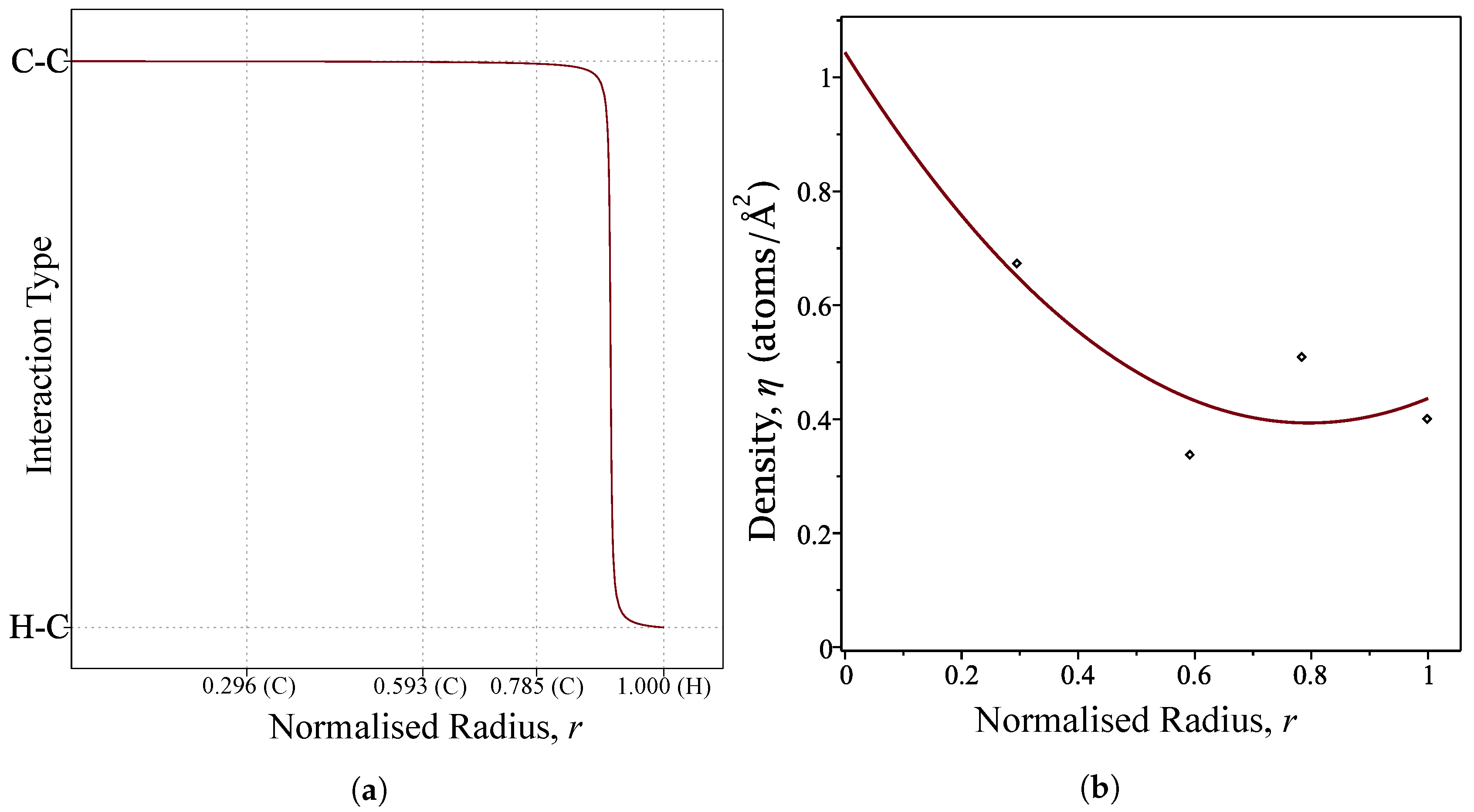
where the Lennard–Jones constants for carbon–carbon and carbon–hydrogen interactions are as given in Table 1 and R is the radius of the coronene molecule, which is taken to be Å [32]. In this paper, we adopt the interaction functions to be in the forms of sigmoidal arctan functions as we assume that the interaction varies similar to a step-function but with smooth transition across the radial direction of the molecule. Specifically, we have
where and are determined using Equation (4). We choose a large value for m in order to mimic the step-function profile, and the value of is chosen to be located between the connection of final carbon atom and the hydrogen atom at the perimeter. Thus, we use and . The profile of the interaction functions is shown in Figure 2a.
2.1. Atomic Density Function
The atomic densities of both surfaces are typically assumed to be uniform, meaning that and are constants and are not included in the integrals, as shown in (1). Here, we assume that the atomic surface density of the coronene molecule is not a constant, i.e., replacing with a function , thus bringing it into the integral along with the interaction functions,
Due to the radial symmetry of the coronene molecule, we also express the atomic density as a function of the radial distance, r. Using the atomic densities calculated in the semi-continuous ring model developed by Tran-Duc et al. [32], a quadratic interpolating polynomial is fitted and used as the atomic density function in our calculation. These densities are presented in Table 2 and the polynomial is plotted in Figure 2b.
To solve the energy integral for a general case, we use
to express the atomic density function, where N here is the degree of the interpolating polynomial.
2.2. Disk and Plane Interaction
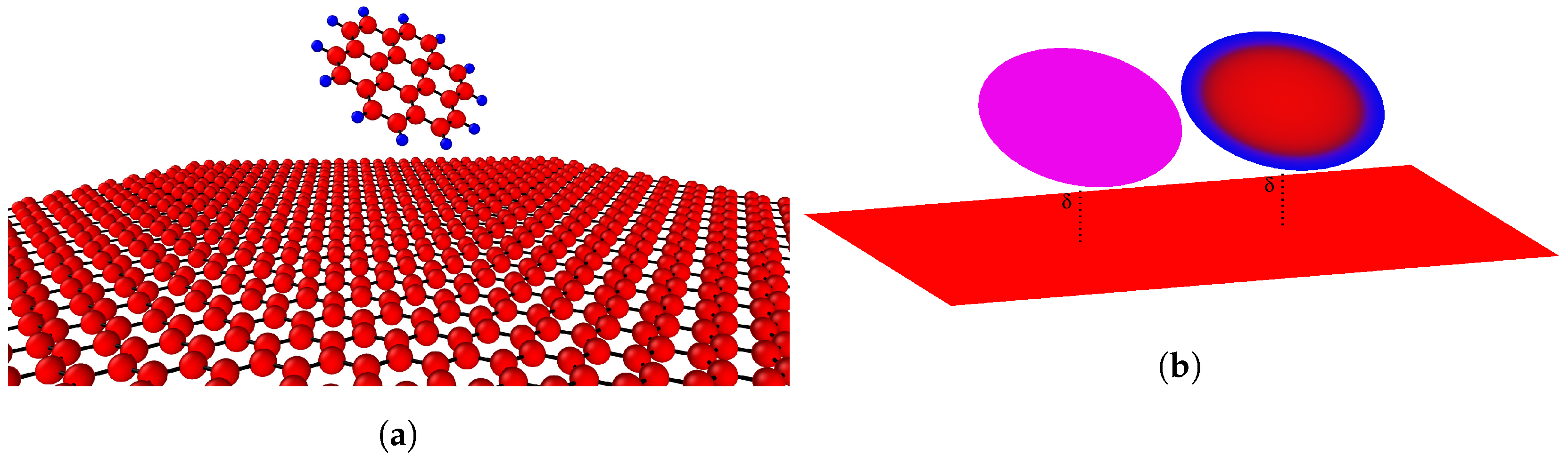
Coronene comprises 24 carbon atoms and 12 hydrogen atoms, arranged in a circular honeycomb structure with carbon atoms in the central region and the hydrogen atoms at the perimeter. Coronene has previously been modeled as concentric rings of carbon and hydrogen atoms [32]. Here, we represent a coronene molecule by a circular disk of radius a centered on the z-axis, and tilted by some angle . We also assume that the centre of the disk is located at a distance away from a sheet of graphene which is assumed to lie flat on the plane.
Next, we define the integral as
where . Evaluating (8), we find that the integral is largely the same as a circular ring interacting with a plane, as the integral in r is independent of the other variables. Thus, we refer the reader to the work of Tran-Duc et al. [32] for detailed computation of most of the integral. The expression for Equation (8) prior to solving the integral in r is
where
Detailed derivation of Equation (10) can be found in Appendix A.
3. Results and Discussion
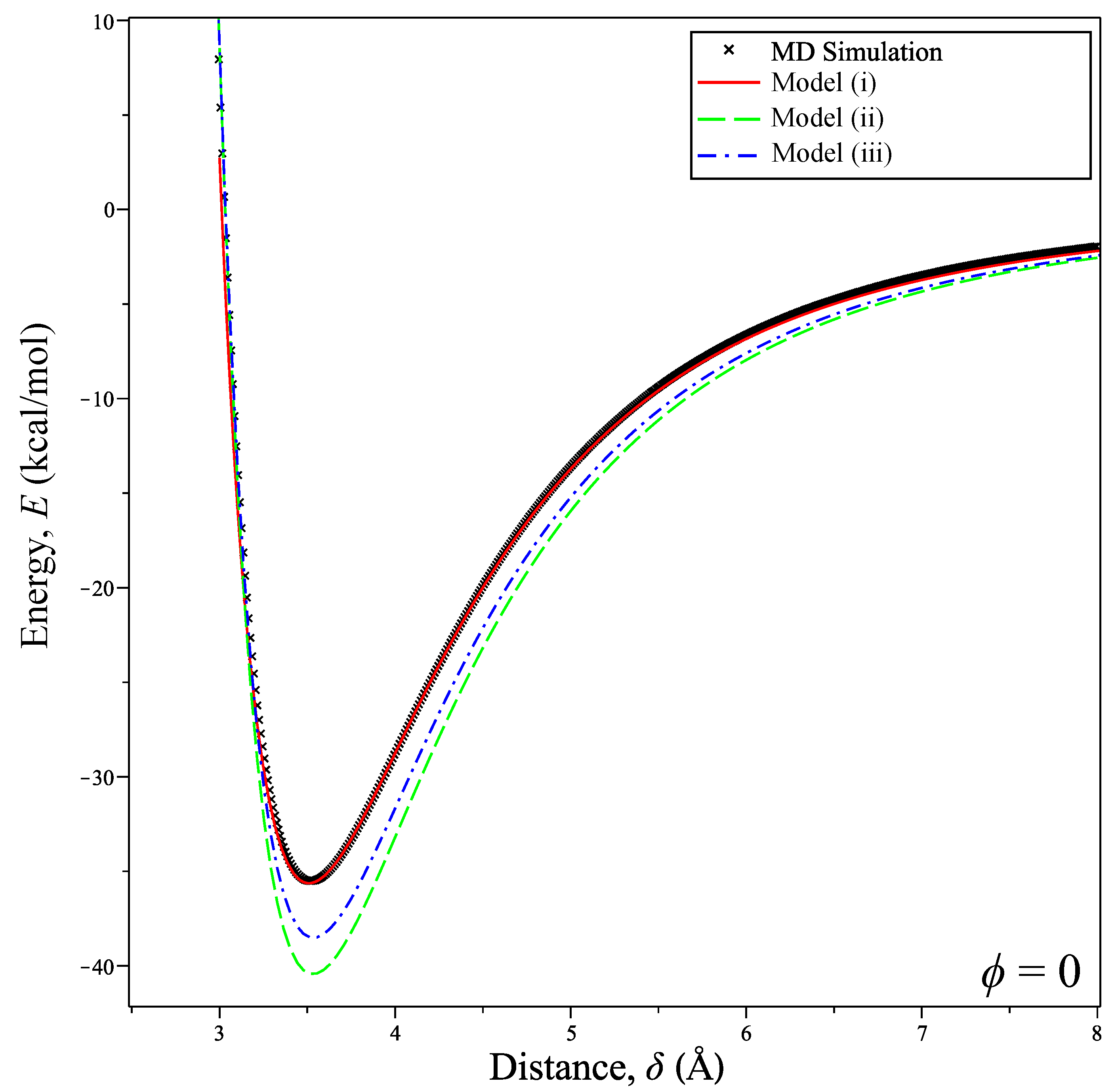
Here, we compare the energies obtained from the three different models: (i) the fully homogeneous disk with constant interaction and density coefficients; (ii) the heterogeneous disk with functional interaction and constant density coefficients; and (iii) the heterogeneous disk with functional interaction and density coefficients, against the results from molecular dynamics (MD) simulations. The MD simulations are performed using the Lennard–Jones potential with a cut-off distance of 14 Å and the graphene sheet used has radius over 20 Å larger than the radius of the coronene molecule ( Å), which justifies the assumption of an infinite plane for the sheet.
Fixing the tilt angle at implies that the coronene molecule lies parallel to the graphene sheet. As seen from Figure 3, the differences in the energy profiles obtained from the three models are obvious. Here, Model (i) agrees excellently with the MD simulation, whereas Models (ii) and (iii) using interaction functions have discrepancies. We find that this is due to Model (i) and the atomistic case being equal when the coronene is parallel to the graphene sheet, which is shown in Appendix B.
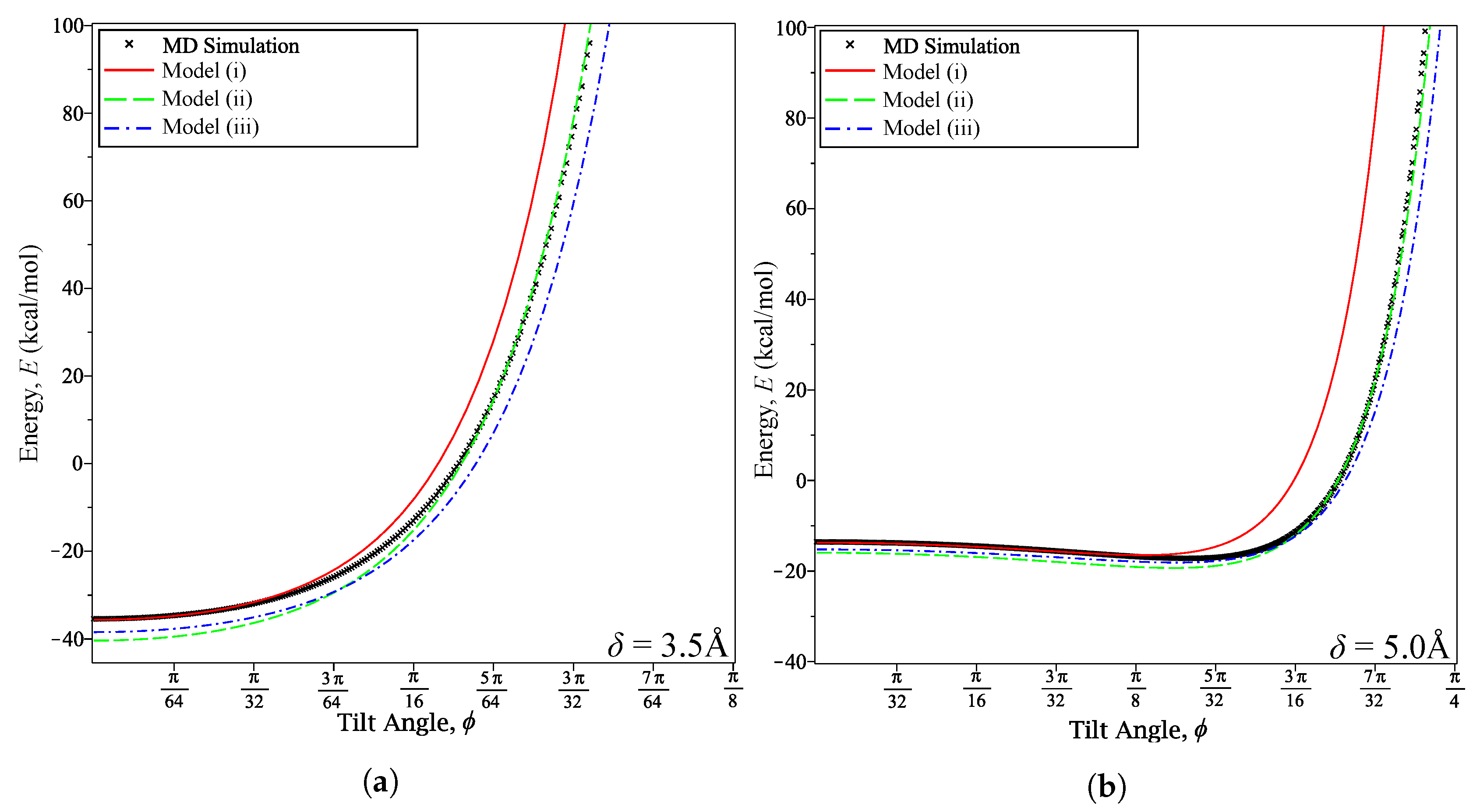
Where Model (i) begins to fail appears to depend on the distance between the coronene and graphene. Figure 4a shows that it fails at when Å and Figure 4b shows that it fails at when 5 Å. Conversely, we notice that Models (ii) and (iii) appear to maintain or increase their accuracy at these fixed distances as increases.
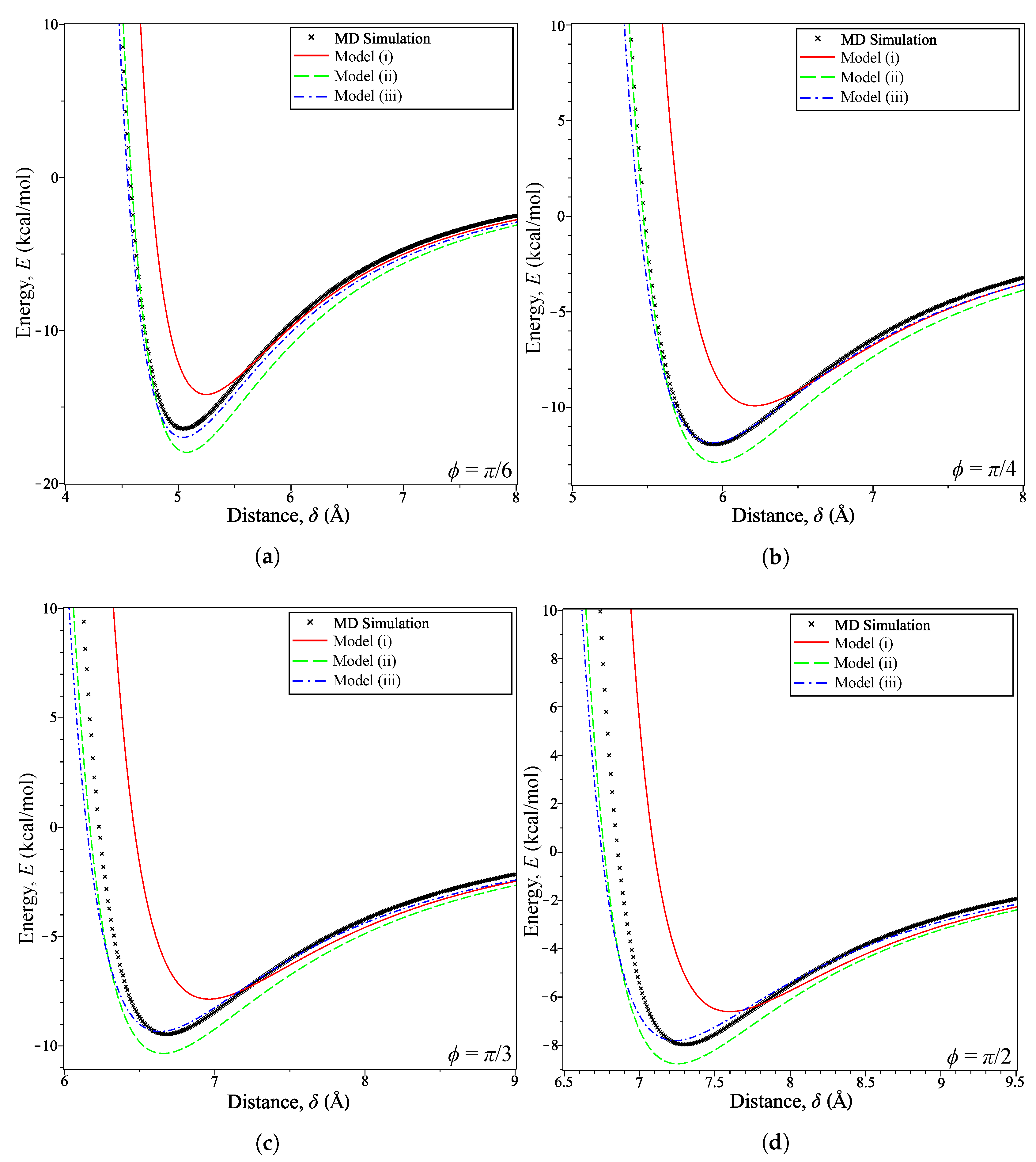
For , we see that Model (i) becomes very inaccurate for where is the distance at which the energy is minimized . This can be seen in Figure 5 for various values of . Model (ii) produces energy curves that are clearly an improvement over the homogeneous model, as shown in Figure 5a,b. The minimum energy distances presented in Table 3 show this to be the case as the model is consistently within Å of the MD simulation. This is in contrast to the error between the simulation prediction and Model (i), which is initially small at Å when but very quickly increases to Å by .
The combination of the interaction functions and density function seems to correct the discrepancy in energy estimation. This is shown prominently in Figure 5c,d as Model (iii) follows Model (ii) closely until the distance nears . On calculating the error, at each tilt angle we find that this error for the homogeneous Model (i) decreases from at to at An improved error is obtained for Model (ii), for which at to at However, Model (iii) gives the smallest error over this range of tilt angles with at to at The error values in and for the three models indicate that including an interaction function (Model (ii)) increases the accuracy over the purely homogeneous model (Model (i)), which is improved upon further by incorporating a density function (Model (iii)). Thus, unless the coronene molecule alignment is perfectly parallel to the graphene sheet, the homogeneous model of coronene should not be adopted.
4. Conclusions
While the models presented here do not perfectly match the MD results for the energy of the coronene–graphene interaction, it is clear that the fully homogeneous Model (i) gives the largest error in most configurations. Our proposed method could lead to a study to improve the homogeneous models used for the interactions involving a much more complex molecular structures than the coronene molecule. The introduction of simple functions to approximate the interaction strengths and the atomic densities will likely lead to improved energy estimations, which will be the subject of future research.
Author Contributions
Conceptualization, K.S., N.T. and T.T.-D.; methodology, K.S., N.T. and T.T.-D.; software, K.S. and T.T.-D.; validation, K.S.; formal analysis, K.S., N.T. and T.T.-D.; investigation, K.S.; resources, K.S., N.T. and T.T.-D.; data curation, K.S.; writing—original draft preparation, K.S.; writing—review and editing, N.T., T.T.-D. and J.M.H.; visualization, K.S.; supervision, N.T., T.T.-D. and J.M.H.; project administration, N.T.; funding acquisition, N.T. All authors have read and agreed to the published version of the manuscript.
Funding
This research was funded by the Australian Research Council, Discovery Project DP170102705.
Acknowledgments
The authors acknowledge the support from the School of Mathematical and Physical Sciences, Faculty of Science at the University of Newcastle. The authors are also grateful to the Australian Research Council for the funding of Discovery Project DP170102705.
Conflicts of Interest
The authors declare no conflict of interest.
Abbreviations
The following abbreviations are used in this manuscript:
| LJ | Lennard–Jones |
| MD | Molecular dynamics |
Appendix A. Evaluation of the Integral I Defined by (10)
To evaluate the integral (10), we use the interaction function . We need to compute
The second part is easily evaluated since For the first part, we make the substitution in order to make the argument of the arctan function easier to manage,
and now we use the binomial theorem to split up the polynomial term in u into the series,
From [33], we have,
and the second integral has two possible forms depending on whether m is even or odd. For m odd, we obtain
while, for m even, we obtain
To make use of these forms, we split the finite sum in Equation (A2) into two sums of odd and even powers,
so that, on applying the integral (A3) and noting that there are no singularities over the interval, we obtain
We then apply (A4) to deduce
Although this looks complicated, due to the series being finite, the expression is easily computable by any mathematical software package, such as MAPLE™ or Mathematica™.
Including a Density Function
Appendix B. Explanation to Why MODEL (i) Is Accurate at ϕ = 0
In this appendix we show that the energy expression for Model (i) matches the energy expression given by the atomistic model of coronene solely when the tilt angle is zero.
Appendix B.1. Model (i)
is the total number of atoms in coronene with the number of carbon atoms and the number of hydrogen. is the atomic density of coronene and is the surface area of the approximated coronene surface. Thus, the interaction energy between a coronene molecule and a parallel graphene sheet is computed by
where and are the averaged interaction coefficients. At , is invariant in the x and y directions, due to the graphene sheet being assumed infinite. Thus, we have
Appendix B.2. Atomistic Model
The interaction energy between a coronene molecule and a parallel graphene sheet is the sum of the interaction energies between each atom and the graphene sheet,
where is the distance between the kth carbon or hydrogen atom and the graphene sheet.
As with the homogeneous case, at , . Thus,
which is equal to the expression derived from the homogeneous approximation.
References
- Rzepka, M.; Lamp, P.; De la Casa-Lillo, M. Physisorption of hydrogen on microporous carbon and carbon nanotubes. J. Phys. Chem. B 1998, 102, 10894–10898. [Google Scholar] [CrossRef] [Green Version]
- Bénard, P.; Chahine, R. Storage of hydrogen by physisorption on carbon and nanostructured materials. Scr. Mater. 2007, 56, 803–808. [Google Scholar] [CrossRef]
- Ren, H.; Ben, T.; Sun, F.; Guo, M.; Jing, X.; Ma, H.; Cai, K.; Qiu, S.; Zhu, G. Synthesis of a porous aromatic framework for adsorbing organic pollutants application. J. Mater. Chem. 2011, 21, 10348–10353. [Google Scholar] [CrossRef]
- Llanos, J.; Fertitta, A.; Flores, E.; Bottani, E. SO2 physisorption on exfoliated graphite. J. Phys. Chem. B 2003, 107, 8448–8453. [Google Scholar] [CrossRef]
- Steinmüller-Nethl, D.; Kloss, F.R.; Najam-Ul-Haq, M.; Rainer, M.; Larsson, K.; Linsmeier, C.; Köhler, G.; Fehrer, C.; Lepperdinger, G.; Liu, X.; et al. Strong binding of bioactive BMP-2 to nanocrystalline diamond by physisorption. Biomaterials 2006, 27, 4547–4556. [Google Scholar] [CrossRef] [PubMed]
- Wang, H.; Ceulemans, A. Physisorption of adenine DNA nucleosides on zigzag and armchair single-walled carbon nanotubes: A first-principles study. Phys. Rev. B 2009, 79, 195419. [Google Scholar] [CrossRef]
- Ulbricht, H.; Moos, G.; Hertel, T. Physisorption of molecular oxygen on single-wall carbon nanotube bundles and graphite. Phys. Rev. B 2002, 66, 075404. [Google Scholar] [CrossRef] [Green Version]
- Smith, D.G.; Patkowski, K. Toward an accurate description of methane physisorption on carbon nanotubes. J. Phys. Chem. C 2014, 118, 544–550. [Google Scholar] [CrossRef]
- Vela, S.; Huarte-Larra naga, F. A molecular dynamics simulation of methane adsorption in single walled carbon nanotube bundles. Carbon 2011, 49, 4544–4553. [Google Scholar] [CrossRef]
- Hentschke, R.; Schürmann, B.L.; Rabe, J.P. Molecular dynamics simulations of ordered alkane chains physisorbed on graphite. J. Chem. Phys. 1992, 96, 6213–6221. [Google Scholar] [CrossRef]
- Qin, Q.; Sun, T.; Wang, H.; Brault, P.; An, H.; Xie, L.; Peng, Q. Adsorption and diffusion of hydrogen in carbon honeycomb. Nanomaterials 2020, 10, 344. [Google Scholar] [CrossRef] [PubMed] [Green Version]
- Hu, B.; Gao, Z.; Wang, H.; Wang, J.; Cheng, M. Computational insights into the sorption mechanism of polycyclic aromatic hydrocarbons by carbon nanotube through density functional theory calculation and molecular dynamics simulation. Comput. Mater. Sci. 2020, 179, 109677. [Google Scholar] [CrossRef]
- Darkrim, F.; Levesque, D. Monte Carlo simulations of hydrogen adsorption in single-walled carbon nanotubes. J. Chem. Phys. 1998, 109, 4981–4984. [Google Scholar] [CrossRef]
- Gatica, S.M.; Nekhai, A.; Scrivener, A. Adsorption and gas separation of molecules by carbon nanohorns. Molecules 2016, 21, 662. [Google Scholar] [CrossRef] [Green Version]
- Thornton, A.W. Mathematical Modelling of Gas Separation and Storage Using Advanced Materials. Ph.D. Thesis, University of Wollongong, Wollongong, Australia, 2009. [Google Scholar]
- Adisa, O.O.; Cox, B.J.; Hill, J.M. Encapsulation of methane in nanotube bundles. Micro Nano Lett. 2010, 5, 291–295. [Google Scholar] [CrossRef]
- Adisa, O.O.; Cox, B.J.; Hill, J.M. Encapsulation of methane molecules into carbon nanotubes. Phys. B Condens. Matter 2011, 406, 88–93. [Google Scholar] [CrossRef]
- Tran-Duc, T.; Thamwattana, N.; Baowan, D. Modelling gas storage capacity for porous aromatic frameworks. J. Comput. Theor. Nanosci. 2014, 11, 234–241. [Google Scholar] [CrossRef]
- Stevens, K.; Tran-Duc, T.; Thamwattana, N.; Hill, J. Continuum Modelling for Interacting Coronene Molecules with a Carbon Nanotube. Nanomaterials 2020, 10, 152. [Google Scholar] [CrossRef] [Green Version]
- Garalleh, H.A.; Thamwattana, N.; Cox, B.J.; Hill, J.M. Encapsulation of L-Histidine amino acid inside single-walled carbon nanotubes. J. Biomater. Tissue Eng. 2016, 6, 362–369. [Google Scholar] [CrossRef]
- Thamwattana, N.; Sarapat, P.; Chan, Y. Mechanics and dynamics of lysozyme immobilisation inside nanotubes. J. Phys. Condens. Matter 2019, 31, 265901. [Google Scholar] [CrossRef]
- Thamwattana, N.; Baowan, D.; Cox, B.J. Modelling bovine serum albumin inside carbon nanotubes. RSC Adv. 2013, 3, 23482–23488. [Google Scholar] [CrossRef] [Green Version]
- Tran-Duc, T.; Thamwattana, N.; Hill, J.M. Orientation of a benzene molecule inside a carbon nanotube. J. Math. Chem. 2011, 49, 1115–1127. [Google Scholar] [CrossRef]
- Hilder, T.A.; Hill, J.M. Modelling the encapsulation of the anticancer drug cisplatin into carbon nanotubes. Nanotechnology 2007, 18, 275704. [Google Scholar] [CrossRef]
- Chan, Y.; Hill, J. Modelling interaction of atoms and ions with graphene. Micro Nano Lett. 2010, 5, 247–250. [Google Scholar] [CrossRef] [Green Version]
- Sarapat, P.; Hill, J.M.; Baowan, D. Mechanics of atoms interacting with a carbon nanotorus: Optimal configuration and oscillation behaviour. Philos. Mag. 2019, 99, 1386–1399. [Google Scholar] [CrossRef]
- Baowan, D.; Cox, B.J.; Hilder, T.A.; Hill, J.M.; Thamwattana, N. Modelling and Mechanics of Carbon-Based Nanostructured Materials, 1st ed.; William Andrew: Norwich, NY, USA, 2017. [Google Scholar]
- Girifalco, L.A. Molecular properties of fullerene in the gas and solid phases. J. Phys. Chem. 1992, 96, 858–861. [Google Scholar] [CrossRef]
- Alshehri, M.H.; Cox, B.J.; Hill, J.M. DNA adsorption on graphene. Eur. Phys. J. D 2013, 67, 226. [Google Scholar] [CrossRef]
- Rahmat, F.; Thamwattana, N.; Cox, B.J. Modelling peptide nanotubes for artificial ion channels. Nanotechnology 2011, 22, 445707. [Google Scholar] [CrossRef]
- Stevens, K.; Thamwattana, N.; Tran-Duc, T. New functional Lennard-Jones parameters for heterogeneous molecules. J. Appl. Phys. 2020, 128, 204301. [Google Scholar] [CrossRef]
- Tran-Duc, T.; Thamwattana, N.; Cox, B.J.; Hill, J.M. Adsorption of polycyclic aromatic hydrocarbons on graphite surfaces. Comput. Mater. Sci. 2010, 49, S307–S312. [Google Scholar] [CrossRef]
- Gradshteyn, I.S.; Ryzhik, I.M. Table of Integrals, Series, and Products; Academic Press: Cambridge, MA, USA, 2014. [Google Scholar]
Figure 1.
(a) Atomistic model of interaction; and (b) homogeneous continuous and heterogeneous continuous models.
Figure 1.
(a) Atomistic model of interaction; and (b) homogeneous continuous and heterogeneous continuous models.

Figure 2.
(a) Profile of the interaction function over the normalised radius of the coronene molecule where (C) and (H) denote the location of a carbon and hydrogen atoms, respectively; and (b) profile of the density function over the normalised radius of the coronene molecule.
Figure 2.
(a) Profile of the interaction function over the normalised radius of the coronene molecule where (C) and (H) denote the location of a carbon and hydrogen atoms, respectively; and (b) profile of the density function over the normalised radius of the coronene molecule.

Figure 3.
Calculated potential energy between coronene and graphene at a tilt angle compared with MD simulation.
Figure 3.
Calculated potential energy between coronene and graphene at a tilt angle compared with MD simulation.

Figure 4.
Energy curves at various fixed δ for varying ϕ: (a) δ = 3.5 Å; and (b) δ = 5 Å.

Figure 5.
Energy profiles for coronene at fixed tilt angles: (a) ; (b) ; (c) ; (d) .


Table 1.
Attractive and repulsive constants for carbon–carbon and carbon–hydrogen interactions.
| Interaction | ||
|---|---|---|
| Carbon–Carbon | 112,175,566 | |
| Carbon–Hydrogen | 91,727.95 |
Table 2.
Atomic density values at particular radii [32].
Table 2.
Atomic density values at particular radii [32].
| Radius (Å) | Normalised Radius r | Density () |
|---|---|---|
Table 3.
Various minimum energies and corresponding displacements for the coronene–graphene interactions.
Table 3.
Various minimum energies and corresponding displacements for the coronene–graphene interactions.
| Model | (Å) | () | |
|---|---|---|---|
| (i) | 0 | ||
| (ii) | 0 | ||
| (iii) | 0 | ||
| MD Simulation | 0 | ||
Publisher’s Note: MDPI stays neutral with regard to jurisdictional claims in published maps and institutional affiliations. |
© 2020 by the authors. Licensee MDPI, Basel, Switzerland. This article is an open access article distributed under the terms and conditions of the Creative Commons Attribution (CC BY) license (http://creativecommons.org/licenses/by/4.0/).
Share and Cite
MDPI and ACS Style
Stevens, K.; Tran-Duc, T.; Thamwattana, N.; Hill, J.M. Modeling Interactions between Graphene and Heterogeneous Molecules. Computation 2020, 8, 107. https://0-doi-org.brum.beds.ac.uk/10.3390/computation8040107
AMA Style
Stevens K, Tran-Duc T, Thamwattana N, Hill JM. Modeling Interactions between Graphene and Heterogeneous Molecules. Computation. 2020; 8(4):107. https://0-doi-org.brum.beds.ac.uk/10.3390/computation8040107
Chicago/Turabian StyleStevens, Kyle, Thien Tran-Duc, Ngamta Thamwattana, and James M. Hill. 2020. "Modeling Interactions between Graphene and Heterogeneous Molecules" Computation 8, no. 4: 107. https://0-doi-org.brum.beds.ac.uk/10.3390/computation8040107
Note that from the first issue of 2016, this journal uses article numbers instead of page numbers. See further details here.