
Effect of Additional Order in Two-Stage Supply Chain Contract under the Demand Uncertainty

1
Department of Mathematics, Faculty of Science, Mahidol University, Bangkok 10400, Thailand
2
Centre of Excellence in Mathematics, CHE, Bangkok 10400, Thailand
*
Author to whom correspondence should be addressed.
Computation 2021, 9(3), 37; https://0-doi-org.brum.beds.ac.uk/10.3390/computation9030037
Submission received: 1 March 2021
/
Revised: 19 March 2021
/
Accepted: 19 March 2021
/
Published: 22 March 2021
(This article belongs to the Special Issue Proceedings of the International Conference in Mathematics and Applications 2020_Mahidol University)
Abstract
:In this work, mathematical models are formulated in order to investigate the effect of the additional order on the expected total profit of a two-stage supply chain. A multi-period buyback contract between a supplier and a retailer under the demand uncertainty is considered. Under the contract, an advance order is submitted to the supplier in advance when the demand is unknown, and an additional order can be made at the beginning of each period after the previous period demand is realized. The impact of the coordination on the supply chain’s expected total profit is also considered. The results show that the additional order does not always increases the supply chain profit. The additional order increases the supply chain profit only when both the retailer and supplier are coordinated. Under the decentralized system with the buyback contract, the retailer tends to order less in an advance order to reduce the risk. This leads to the higher cost due the additional order after the demand is realized. As a result, it is lowers the supply chain profit. Moreover, the sensitivity analysis is performed using numerical studies in order to observe the behavior of the expected total profit of the supply chain.
1. Introduction
Every company in the supply chain needs to achieve its own goal, which is to satisfy the customer’s demand while maximizing profit or minimizing costs. Maximizing profit for only individual companies may not be maximizing the supply chain’s profit. To optimize the supply chain’s profit, efficient coordination between companies in the supply chain is needed. A contract is one of the strategies to enable coordination in the supply chain. The partners in the contract get the additional benefits together. For example, a retailer can be sure that there are enough products available to sell to customers and the products can be obtained at an acceptable price, while a supplier will be able to plan the production accordingly.
The contracts are widely studied to consider the channel coordination of the supply chain. Many kinds of contracts have been investigated in the literature. It was shown by Chui et al. that the combined contract consists of the wholesale price, channel rebate, and returns contracts can coordinate a supply chain [1]. Xiong et al. proposed a composite contract by combining a buyback contract and a quantity flexibility contract for one period [2]. They have found that the composite contract is more flexible in terms of supply chain coordination, profit allocation, and risk allocation than the buyback and the quantity flexibility contracts. Sana investigated the coordination under the demand that is sensitive to promotional effort for a single period leading to the discovery that the return/buyback policy can stimulate the retailer to order more and the discount on wholesale price can motivate both parties to achieve their profits [3]. Chui et al. later considered a two-stage supply chain with a manufacturer and multiple heterogeneous retailers as well as two options of the target sales rebate contract with a fixed order quantity and the target sales rebate contract with a minimum order quantity and quantity discount [4]. They found that the supply chain coordination could be achieved in the contract. The manufacturer can maximize its expected profit only if the expected profit of the supply chain is maximized. Doganoglu and Inceoglu considered two different industry structures, first with a vertically integrated manufacturer and an independent retailer, second with an upstream only manufacturer and two competing retailers, to provide an additional reason for the prevalence of buyback provisions in wholesale contracts [5]. They show that a buyback contract in this respect has a function similar to insurance for the retailers; then, this feature may enable the manufacturer to obtain maximum industry profits.
Moreover, the impact of the ordering types on the supply chain coordination has been considered. Cachon considered the pull contract, the push contract, and the advance-purchase discount contract (APD) for a single selling season in order to study the inventory risk allocation and the profit division in the contract [6]. The APD contract has two types of ordering with two wholesale prices. With the first type, the order with a discounted price is submitted before starting the selling season. With the second type, the order with a regular price is submitted during the selling season. He and Zhao analyzed the behavior of an APD contract for a selling season and found that the APD with a revenue sharing contract could coordinate the supply chain with both supply and demand uncertainties as well as achieve flexible profit allocation [7]. Zhang et al. investigated the retailer’s ordering policy having two ordering opportunities, that is, before and during the selling season [8]. An advance payment is required in securing a stable supply source when the order is placed before the selling season. Their work shows that the advance payment is positively related to the variance of the supply rate, and the advance payment is increased along with the supply risk.
In addition, many works have been involved with the study of a multi-period contract in order to optimize the benefit of the supply chain in both decentralized and centralized systems. Xu considered a multi-period dynamic supply contract with the order being placed by the buyer in each period, allowing the cancellation of a portion of an order with penalty [9]. They showed that the dynamic cancellation contract could not achieve channel coordination. Zou et al. considered the two-period contract models under the decentralized and centralized systems [10]. They formulated the models by the dynamic programming and found that adjusting both the wholesale price and buyback price could coordinate the supply chain under the decentralized system. Lain and Deshmukh investigated a quantity flexibility contract, giving a buyer discounts for advance purchase commitment and allowing the increase of the order quantities for future periods with higher unit cost [11]. They proposed a finite-horizon dynamic programming model and developed two heuristic approaches in order to derive a good ordering policy to minimize the total expected cost. Linh and Hong studied two models under the revenue sharing contract in a two-period newsboy problem, namely, a single-buying-opportunity model for products with long lead times and a two-buying-opportunity model for products with short lead times [12]. They found the wholesale prices to be set lower than the retail prices and the optimal revenue sharing ratio to be linearly increasing in the wholesale prices. Hematyar and Chaharsooghi proposed an insurance contract between one manufacturer and one retailer in a two-period newsboy problem and compared the contract with the revenue sharing contract. The results show that the insurance contract can coordinate the supply chain and improve the expected profit of the supplier [13]. Park and Kim considered a multi-period capacity reservation contract between a retailer and several heterogeneous suppliers in order to determine the order quantities in the current period as well as revise the reservation quantity for a contracted period [14].
Under the contract, the retailer will submit the order in advance in order to get some benefit, for example, the discounted wholesale price, the buyback price for the remaining inventory, and to ensure that the order quantity is fulfilled. Then, the supplier gets the information from the advance order and is able to plan the production capacity. The additional order that is allowed to be made in the selling period impacts on the supply chain, as mentioned in [6,7,8]. In addition, the long-term contracts between the supplier and the retailer may help reduce any risks and manage the ordering and production systems more efficiently. Thus, this work studies a multi-period buyback contract between a supplier and a retailer under the demand uncertainty in order to investigate the effect of the additional order on the supply chain’s expected total profit. This work is closest to the works by Zou et al. [10] and He and Zhao [7]. Zou et al. provided the optimal production and/or purchasing quantity in each period. However, they have not obtained the advance quantities for a multi-period contract [10]. He and Zhao considered the advance-purchase discount contract allowing two order opportunities under the uncertainty of supply and demand for a single period only [7].
In this work, the multi-period buyback contract between one supplier and one retailer under the demand uncertainty is considered. The expected total profits from a multi-period buyback contract are formulated for the decentralized and centralized systems in order to study the impact of channel coordination through the contract. In addition, the expected total profits of the supply chain are formulated under three models, which are the model with advance order only, the model with additional order only, and the model with advance-additional orders, to investigate the effect of the additional order on the supply chain’s profit.
2. Model Formulation
Mathematical models are constructed with the expected total profit of the supply chain under the uncertainty demand for a multi-period buyback contract between one supplier and one retailer. The supply chain’s profits are considered under three ordering policies to investigate the effect of the additional order. The three ordering policies consist of the advance order only, the additional order only, and the advance-additional orders policies. Moreover, the profits are formulated for both decentralized and centralized systems to consider the impact of the coordination.
2.1. Problem Descriptions and Assumptions
A two-stage supply chain consisting of one supplier and one retailer is considered. Both the supplier and the retailer agree to the contract, for which the decisions on order quantities, wholesale price, and buyback price for some certain periods must be determined. The plans for these periods are referred to as the horizontal planning. At the beginning of the horizontal planning, the retailer makes the decision on the advance order for each period when the demand is uncertain. Then, once the demand for each period is realized, the retailer determines the additional order (if it is allowed) for the next period in order to adjust their inventory. The order quantities are replenished at the beginning of each selling period with no lead time. At the end of the horizontal planning, the supplier pays the buyback price for the retailer’s leftovers but no more than the total advance order quantities, and the unsatisfied demand is a lost sale. The notations and the assumptions in the problem are the followings.
2.1.1. Notations
The parameters and variables in the models are defined as follows.
| Parameter | |
| unit selling price that the retailer charges the end customer | |
| unit holding cost of the retailer for the remaining inventory at the end of each period | |
| unit shortage cost of the retailer for the unsatisfied demand at the end of each period | |
| unit production cost of the supplier | |
| initial inventory of the retailer at the beginning of planning horizon; | |
| remaining inventory of the retailer at the end of period | |
| unsatisfied demand of the retailer at the end of period | |
| identical independent demand random variable of period ; , | |
| realized demand of period | |
Then, we let be the probability density function of demand , and is the cumulative distribution function of demand .
The decision variables in the models are defined as follows.
| Decision variable | |
| unit wholesale price for advance order quantity | |
| unit wholesale price for additional order quantity | |
| unit buyback price that the supplier pays to the retailer for the leftover at the end of the horizontal planning | |
| advance order quantity at period | |
| additional order quantity at period | |
Under the multi-period buyback contract, the retailer makes the decision on and , and the supplier makes a decision on , , and under the decentralized system. For centralized system, the retailer and the supplier are coordinated.
2.1.2. Assumptions
The assumptions of the problem are as follows.
- The problem under a multi-period buyback contract is studied for two periods.
- The supplier produces a single product under the make-to-order process.
- The advance and the additional orders are replenished at the beginning of each selling period with no lead time.
- There is no backorder at the beginning of the planning horizon; that is, the initial inventory is non-negative, .
- The remaining inventory at the end of period can be sold in the next period.
- The supplier pays the unit buyback price for the retailer’s leftovers but no more than the total order quantities.
- The unsatisfied demand at the end of the horizontal planning is a lost sale.
- The unit wholesale price for the additional order is greater than the unit wholesale price for the advance order but less than the unit selling price, .
- The unit production cost includes the operation and transportation costs.
To obtain the optimal policy shown in Section 3, the expected total profit for each model is firstly determined and the optimal advance orders can be obtained by maximizing the total profits. To determine the optimal additional orders , the dynamic programming approach is considered.
In the following, the expected total profit of the supply chain for each model is obtained under the decentralized and the centralized systems, respectively.
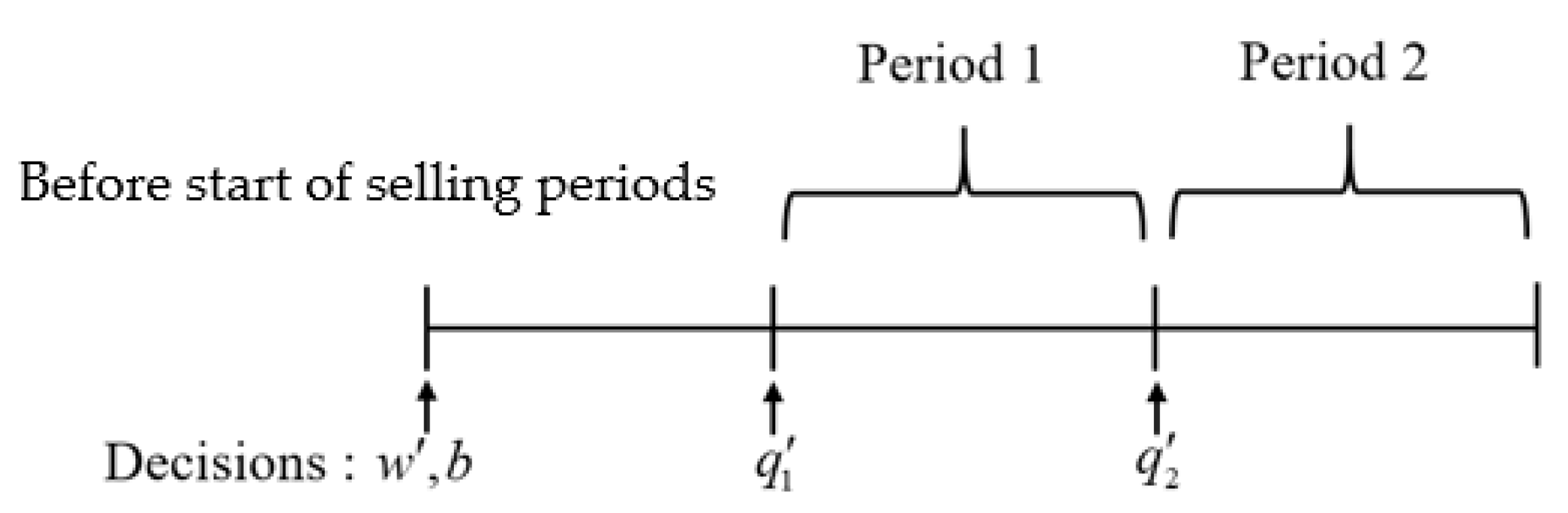
2.2. Model 1: Advance Order Only
For Model 1, the retailer submits only the order quantities in advance long before the beginning of the selling periods. The timeline of decision making is shown in Figure 1. The expected total profits of the supply chain are provided under the decentralized and the centralized systems, respectively.
2.2.1. Decentralized System
In Model 1, the expected total profits of the retailer and the supplier under the decentralized system are given as in Lemmas 1 and 2.
Lemma 1.
For a two-period buyback contract with advance order only, the retailer’s expected total profitunder the decentralized system is given by
Proof:
The retailer’s profit can be divided into six cases.
Case 1: There is no shortage in periods 1 and 2 and the supplier buys back all inventory. The profit is
Case 2: There is no shortage in periods 1 and 2 and the supplier buys back up to the total of order quantities. The profit is
Case 3: There is a lost sale in period 2. The profit is
Case 4: There is a shortage in period 1 and the supplier buys back all inventory. The profit is
Case 5: There is a shortage in period 1 and the supplier buys back up to the total of order quantities. The profit is
Case 6: There is a shortage in period 1 and a lost sale in period 2.
The expected total profit is given by
which can be simplified as shown in Equation (1). □
Lemma 2.
For a two-period buyback contract with advance order only, the supplier’s expected total profitunder the decentralized system is given by
Proof:
The proof is similar to the proof shown in Lemma 1. □
From Lemmas 1 and 2, the expected total profit of the supply chain can be given as
2.2.2. Centralized System
In Model 1, the expected total profit of the supply chain under the centralized system can be found by considering the profits of the retailer and the supplier together. This is provided by Lemma 3.
Lemma 3.
For a two-period buyback contract with advance order only, the supply chain’s expected total profitunder the centralized system is given by
Proof:
The proof is similar to the proof shown in Lemma 1. □
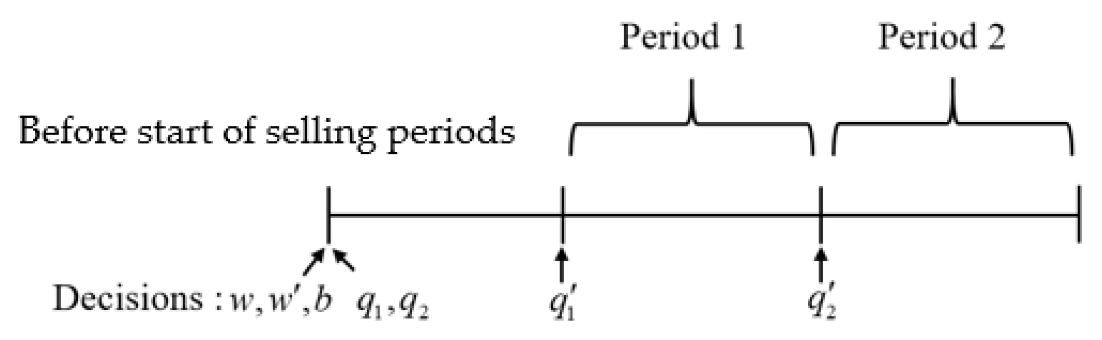
2.3. Model 2: Additional Order Only
For Model 2, the retailer places the additional order, which is the order quantity just before the beginning of each selling period. Making a decision on the additional order depends on the state of the inventory level at the beginning of the period. Dynamic programming is used to find the additional ordering policy. The timeline of decision making is shown in Figure 2. The expected total profits of the supply chain for both decentralized and centralized systems are presented in what follows.
2.3.1. Decentralized System
In Model 2, the retailer makes the decisions on additional order at the beginning of each period after the demand of previous periods are realized. In this case, the dynamic programming approach is used to determine the optimal inventory level for each period.
The expected total profits of the retailer and the supplier can be formulated as shown in Lemmas 4 and 5.
Lemma 4.
For a two-period buyback contract with additional order only, the retailer’s expected total profitunder the decentralized system is given by
Proof:
The additional order in period depends on the inventory level at the beginning of period before ordering , the states of period are composed of the on-hand inventory and the unsatisfied demand , . Since and cannot occur at the same time, then the state of each period is either or . That is, represents a state in which there is on-hand inventory at the beginning of period , , and is the state where there exists the backlog units from the previous period, .
The backward approach is considered to solve the problem. That is, the expected profit of each state in period 2 is obtained first, and then period 1 is considered, respectively. The optimal inventory level for period 1 is and the optimal inventory level for period 2 is . Using these results, the expected total profit for the retailer can be obtained as shown in Equation (5). □
Using the results obtained the proof in Lemma 4. The supplier’s expected total profit can be obtained as shown in the following lemma.
Lemma 5.
For a two-period buyback contract with additional order only, the supplier’s expected total profitunder the decentralized system is given by
Lemma 6.
For a two-period buyback contract with additional order only, the supply chain’s expected total profitunder the decentralized system is given by
Proof:
The proof is similar to the proof shown in Lemma 4. □
2.3.2. Centralized System
In Model 2, the expected total profit of the supply chain under the centralized system is derived from the backward dynamic programming. The states of each period are considered in the similar manner as the decentralized system. Using the additional ordering policy under the centralized system, the expected total profit of the supply chain is derivable under conditions that involve the optimal inventory level at the beginning of period 1, period 2, and
Now, we let . The expected total profit of the supply chain can be formulated as shown in Lemma 7.
Lemma 7.
For a two-period buyback contract with additional order only, the supply chain’s expected total profitunder the centralized system is given by
2.4. Model 3: Advance-Additional Orders
For Model 3, the retailer makes decisions on the advance order when demand information is highly uncertain. Then, once the demand in each period is realized, the retailer is allowed to place the additional order for the next period with the higher wholesale price at the beginning of each selling period. The timeline of decision making is shown in Figure 3.
The problem can be formulated using a stochastic programming. We solve for the optimal solution backward. First, dynamic programming is used to obtain the additional ordering policy. The additional order is taken into account to derive the expected total profit, and then, the advance ordering policy is obtained.
2.4.1. Decentralized System
In Model 3, the advance orders are submitted before the retailer makes a decision on the additional order. Therefore, the state of period is or where is the on hand inventory at the beginning of period after receiving but before ordering ;
Similarly, the back-order state
Since the submitted advance order is optimal under the unknown demand , let be considered. The expected total profits of the retailer and the supplier are provided by the following.
Lemma 8.
For a two-period buyback contract with advance and additional orders, the retailer’s expected total profitunder the decentralized system is given by
Proof:
Since the retailer must make decisions on both advance and additional orders, the optimal inventory level in period 2 is determined using a similar approach as shown in Lemma 4. Then, the similar approach to the proof shown in Lemma 1 is used to determine the retailer’s expected profit. □
Lemma 9.
For a two-period buyback contract with advance and additional orders, the supplier’s expected total profitunder the decentralized system is given by
Proof:
Use the results obtained in Lemma 8 and apply the similar approach as shown in Lemma 1. □
In Model 3, the expected total profit of the supply chain under the decentralized system can be given by Equation (11),
2.4.2. Centralized System
In Model 3, the ordering policy under the centralized system is derived in the similar way as the decentralized system. The additional ordering policy is obtained by dynamic programming and is taken into account in the expected total profit of the supply chain. Then, the advance ordering policy is obtained. The expected total profit of the supply chain is given by the following.
Lemma 10.
For a two-period buyback contract with advance and additional orders, the supply chain’s expected total profit under the centralized system is given by
Proof:
The proof is similar to the proof shown in Lemma 1 and Lemma 8. □
3. Results
In this section, the optimal ordering policies are obtained and presented for each model based on the expected total profits of the retailer, the supplier, and the supply chain.
3.1. Optimal Advance Ordering Policy in Model 1
In the advance order only model, the retailer submits the orders in advance under the uncertain demand. There are two advance ordering policies, which are obtained from maximizing the expected total profits of the retailer and the supply chain. Although quantities cannot be written explicitly in the closed form for the advance order only, we provide the optimal order conditions as shown in Theorems 1 and 2, which are concerned with the advance ordering policies under the decentralized and the centralized systems, respectively.
Theorem 1.
Letbe the optimal advance order quantity in any periodunder the decentralized system, which maximizes the expected total profit of the retailer and the initial inventory. Under the buyback contract with advance order only, the ordering policyis given bywheremust satisfy the following conditions:
Proof:
From the expected total profit of the retailer in Lemma 1, differentiating both sides of Equation (1) with respect to and , we have
Let for and .
We have the system of equations
From simplifying the above system of equations and the order quantities being necessarily non-negative, the advance orders that maximize the expected total profit of the retailer are , and satisfies Equations (15) and (16):
□
Theorem 2.
Letbe the optimal advance order quantity in any periodunder the centralized system, which maximizes the expected total profit of the supply chain and the initial inventory. Under the buyback contract with advance order only, the ordering policyis given by, wheremust satisfy the following system:
Proof:
The proof is similar to the proof shown in Theorem 1 by considering Lemma 3. □
From Theorems 1 and 2, we obtain the optimal advance order in period 1 and substitute it into another equation in the system. Then, the optimal advance orders for two periods are obtained.
3.2. Optimal Additional Ordering Policy in Model 2
In Model 2, the retailer places the additional orders just before the beginning of each selling period. Dynamic programming is used to provide the additional ordering policy under the decentralized and the centralized systems, which are defined in Propositions 1 and 2.
Proposition 1.
Letbe the optimal additional order in periodunder the decentralized system. Given the inventory at the beginning of period,, or, under a buyback contract with additional order only, the additional ordering policy is as follows:
a. For period 1:
b. For period 2:
Proposition 2.
Letbe the optimal additional order in periodunder the centralized system. Given the inventory at the beginning of period,, or, under a buyback contract with additional order only, the additional ordering policy is as follows:
a. For period 1:
b. For period 2:
From Propositions 1 and 2, the optimal inventory level at the beginning of period , , is provided first, and then the additional order in each period is obtained from the ordering policy.
3.3. Optimal Additional and Advance Ordering Policies in Model 3
In Model 3, the additional orders are determined given that the advance orders are known. Dynamic programming is used to derive the optimal additional orders. Therefore, the state of period is or , where
Similarly, the backorder state
Proposition 3.
Letbe the optimal additional order under the decentralized system in period. Given the inventory at the beginning of period,or, under the buyback contract with advance and additional orders, the additional ordering policy for the retailer is as follows:
a. For period 1:
b. For period 2:
Theorem 3.
The optimal conditions for the advance orders that maximizes the expected total profit of the retailer under the decentralized system,and, follow Equations (19) and (20).
where.
Proof:
Using the result in Proposition 3 to obtain the expected profit, then we can apply the proof which is similar to the proof shown in Theorem 1 by considering Lemma 8. □
Proposition 4.
Letbe the optimal additional order under the centralized system in period. Given the inventory at the beginning of period,, or, under the buyback contract with advance and additional orders, the additional ordering policy for the retailer is as follows:
a. For period 1:
b. For period 2:
Theorem 4
The optimal conditions for the advance orders that maximize the expected total profit of the retailer under the centralized system,and, follow Equations (21) and (22).
where.
Proof:
Using the result in Proposition 4 to obtain the expected profit, then we can apply the proof that is similar to the proof shown in Theorem 1 by considering Lemma 10. □
4. Numerical Study
Due to the complexity of the problem, the optimal order quantities cannot be obtained explicitly. To investigate our further results, a numerical study should be performed. In this section, the numerical study is considered to investigate the effect of the advance and the additional ordering policies on the supply chain’s expected total profit under the two-period buyback contract. Moreover, the initial inventory before starting the horizontal planning is considered to see the changes in decisions and in the supply chain’s expected total profit. The expected total profits are studied in both the decentralized and centralized systems in order to discern the coordination of contracts.
The Weibull distribution is considered as demand distribution in this work. The shape of this Weibull distribution can be varied by adjusting the shape parameter, since the Weibull distribution is a probability density function of continuous random variables that have both symmetric and asymmetric shapes. The probability density function of Weibull distribution is
where is the shape parameter and is the scale parameter of the distribution. When the shape parameter value changes, the Weibull distribution is related to a number of other probability distribution. For example, when , the Weibull distribution becomes exponential distribution, and when , the Weibull distribution becomes the normal distribution.
In this work, we let , , and the buyback price is varied from 0 to 5. In this study, the wholesale price for the additional quantities, , is higher than the wholesale price for the advance quantities, w, that is . The demand subject to Weibull distribution with shape parameter , and the means in period 1 and period 2 are and , respectively.
This section may be divided by subheadings. It should provide a concise and precise description of the experimental results, their interpretation, as well as the experimental conclusions that can be drawn.
4.1. Effect of the Ordering Policies
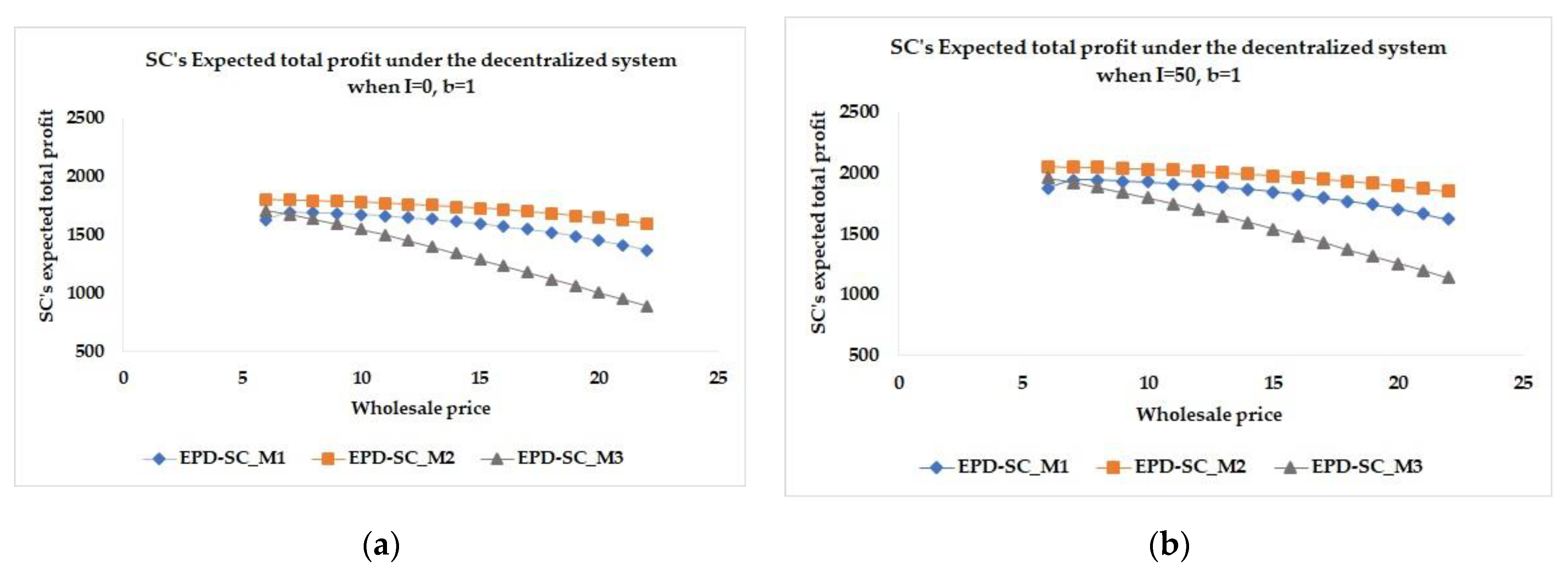
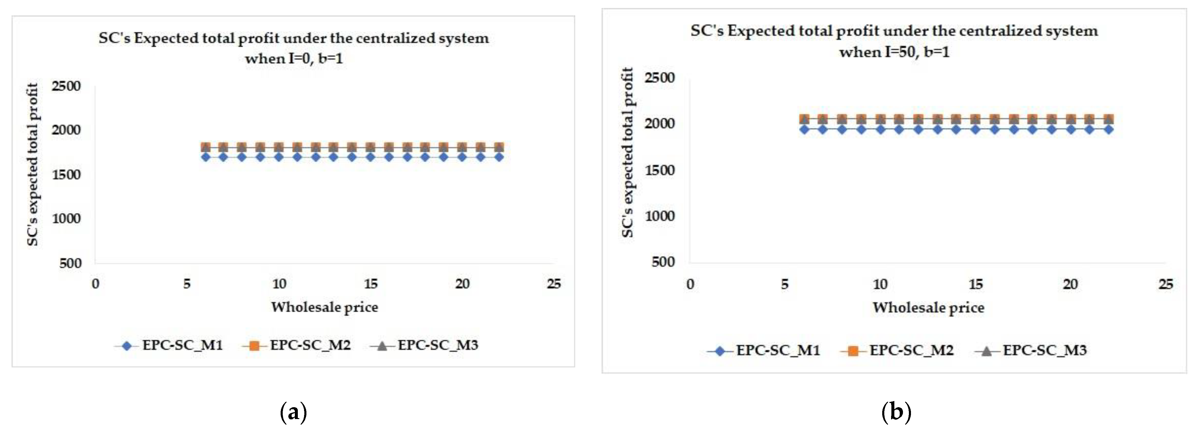
Under the decentralized system, when the buyback price , the supply chain’s expected total profit from an additional order only policy is the greatest, the profit from an advance order only policy is greater than the profit from an advance-additional orders policy for both the initial inventory and , as shown in Figure 4. Furthermore, the results in the cases where are similar to the case when . Under the centralized system, the supply chain’s expected total profits from an additional order only policy and the profit from an advance-additional orders policy are not different. In addition, they are greater than the profit from an advance order only policy, as can be seen in Figure 5.
The results show that the ordering policies with additional orders, that is, the additional order only policy, and the advance-additional orders policy, yield a higher supply chain’s expected total profit than the advance order only policy under the centralized system. In addition, under the decentralized system, the supply chain’s expected total profit from the additional order only policy is the highest.
4.2. Effect of Coordination
The supply chain’s expected total profit under the decentralized system is obtained from the summation of the expected total profit from the perspective of the retailer and the supplier, whereas the expected total profit of the supply chain under the centralized system is obtained from the perspective of the supply chain. The results show that in each model, the supply chain’s expected total profits under the centralized system are greater than or equal to the profits under the decentralized system. In addition, the supply chain’s expected total profit in the case where is less than in the case where , as shown in Table 1. The results in the other case of are similar to the case of . The results in case of are similar to the case of . Therefore, it can be concluded that the coordination under the centralized system and the coordination through the buyback contract affects the expected total profit of the supply chain.
4.3. Sensitivity Analysis
Under the centralized system, the wholesale price and the buyback price are transferred between the supplier and the retailer, so the expected total profit of the supply chain is insensitive with the wholesale price. In the following, the sensitivity analysis is considered in the case of decentralized system.
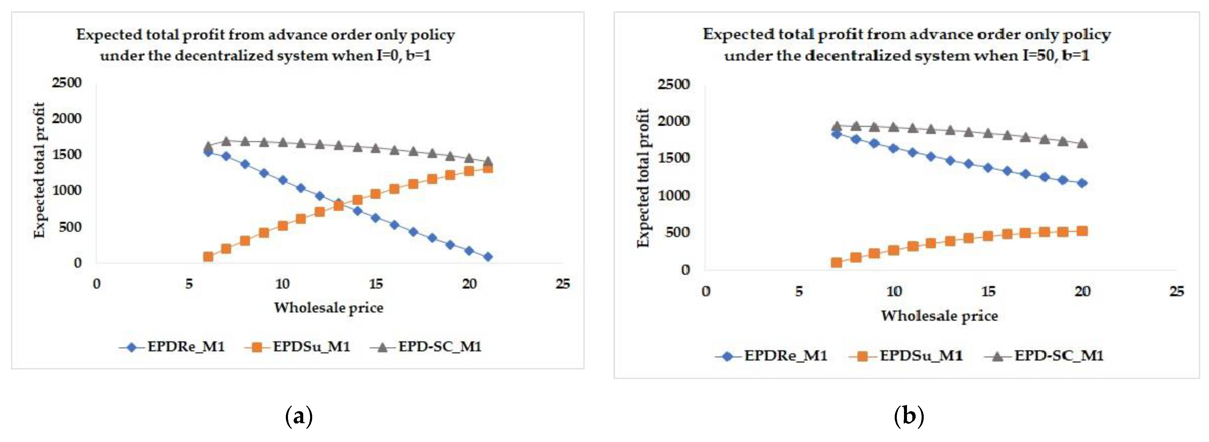
The expected total profits from advance order only, additional order only, and advance-additional orders policies in the case where as shown in Figure 6, Figure 7 and Figure 8, respectively, indicate that as the wholesale price increases, the expected total profit of the retailer decreases but the expected total profit of the supplier increases, whereas the expected total profit of the supply chain decreases. The increase in the wholesale price leads to the increase in the expected total profit of the supplier because is a part of the income of the supplier. On the other hand, is a part of the cost of the retailer, so the expected total profit of the retailer decreases when increases. The results in the case where are similar to the case where . The results in the case where are similar to the case where .
Moreover, the initial inventory affects the expected total profits. The retailer’s expected total profit in the case where is higher than in the case where . Due to the possibility that the retailer may not order the products in some periods, the supplier receives smaller order quantities. The supplier’s expected total profit in the case that is less than in the case that .
5. Conclusions
In this work, a multi-period buyback contract between one supplier and one retailer has been considered under uncertain demand. Mathematical models have been formulated with the expected total profit of the supply chain. In order to investigate the effect of additional orders, the models are formulated under three ordering policies, which are (1) advance order only policy, (2) additional order only policy, and (3) advance-additional orders policy. The expected total profits of the retailer, the supplier, and the supply chain in each model have been obtained under both the decentralized and the centralized systems. Moreover, the optimal ordering policies under the decentralized and the centralized systems in each model have been determined.
The results from the numerical study show that the additional order only policy and the advance-additional orders policy yield a higher supply chain’s expected total profit than the advance order only policy under the centralized system. In addition, under the decentralized system, the supply chain’s expected total profit from the additional order only policy is the highest. Thus, although the retailer needs to pay a higher wholesale price for the additional order quantities, the retailer will gain more profit. Therefore, if the retailer places only one order, then the retailer should place an additional order. In the coordination viewpoint, it can be concluded from the results that coordination do affect the supply chain. That is, the supply chain’s expected total profits in the centralized system are greater than or equal to the profits in the decentralized system, whereas the expected total profit of the supply chain under the buyback contract is greater than in the case of no contract.
In addition, the results indicate that the wholesale price and the buyback price affect the expected total profit of the supply chain under the decentralized system. When buyback prices increase, the expected total profit of the retailer increases. On the other hand, the expected total profit of the supplier decreases when the buyback price increases. Effects of the wholesale price are the opposite; that is, the expected total profit of the supplier increases but the expected total profit of the retailer decreases with the wholesale price. Moreover, the expected total profit of the supply chain under additional order quantities is higher.
There are some limitations on this work. First, our results are based on two periods only. One can investigate more periods. All demands are assumed to be independent, which may not be true in real life. Demand from the previous period can be used to forecast the demand for the next period. Thus, the update forecast can be considered for further research. This work only considers one supplier and one retailer. The work can be extended by considering multiple retailers and/or multiple suppliers. In addition, other types of contracts should be studied.
In this work, the optimal conditions for the ordering policy under the multi-period buyback contract are provided, and the results show that the expected total profits of the supply chain under additional order only and advance-additional orders policies are close to each other under the centralized system. Further work could involve obtaining the optimal advance order quantity and comparing it to the results of additional order only model in order to make a more comprehensive conclusion on the values of additional orders for multiple periods in this supply chain. In addition, studying the model with multiple retailers or multiple suppliers would be the extension to the current results.
Author Contributions
Conceptualization, R.S. and S.C.; methodology, R.S. and S.C.; formal analysis, R.S. and S.C.; resources, S.C. and R.S.; investigation, S.C. and R.S.; writing—original draft preparation, S.C.; writing—review and editing, R.S.; visualization, S.C.; supervision, R.S. All authors have read and agreed to the published version of the manuscript.
Funding
This research received no external funding.
Informed Consent Statement
Not applicable.
Data Availability Statement
All data generated or analysed during this study are included in this published article.
Acknowledgments
This research is (partially) supported by the Centre of Excellence in Mathematics, The Commission on Higher Education, Thailand.
Conflicts of Interest
The authors declare no conflict of interest.
References
- Chiu, C.H.; Choi, T.M.; Tang, C.S. Price, rebate, and returns supply contracts for coordinating supply chains with price-dependent demands. Prod. Oper. Manag. 2011, 20, 81–91. [Google Scholar] [CrossRef]
- Xiong, H.; Chen, B.; Xie, J. A composite contract based on buy back and quantity flexibility contracts. Eur. J. Oper. Res. 2011, 210, 559–567. [Google Scholar] [CrossRef]
- Sana, S.S. Optimal contract strategies for two stage supply chain. Econ. Model. 2013, 30, 253–260. [Google Scholar] [CrossRef]
- Chiu, C.H.; Choi, T.M.; Hao, G.; Li, X. Innovative menu of contracts for coordinating a supply chain with multiple mean-variance retailers. Eur. J. Oper. Res. 2015, 246, 815–825. [Google Scholar] [CrossRef]
- Doganoglu, T.; Inceoglu, F. Buyback contracts to solve upstream opportunism. Eur. J. Oper. Res. 2020, 287, 875–884. [Google Scholar] [CrossRef]
- Cachon, G.P. The allocation of inventory risk in a supply chain: Push, pull, and advance-purchase discount contracts. Manag. Sci. 2004, 50, 222–238. [Google Scholar] [CrossRef] [Green Version]
- He, Y.; Zhao, X. Contracts and coordination: Supply chains with uncertain demand and supply. Nav. Res. Logist. 2016, 63, 305–319. [Google Scholar] [CrossRef]
- Zhang, Q.; Zhang, D.; Tsao, Y.C.; Luo, J. Optimal ordering policy in a two-stage supply chain with advance payment for stable supply capacity. Int. J. Prod. Econ. 2016, 177, 34–43. [Google Scholar] [CrossRef] [Green Version]
- Xu, N. Multi-period dynamic supply contracts with cancellation. Comput. Oper. Res. 2005, 32, 3129–3142. [Google Scholar] [CrossRef]
- Zuo, X.; Pokharel, S.; Piplani, R. A two-period supply contract model for a decentralized assembly system. Eur. J. Oper. Res. 2008, 187, 257–274. [Google Scholar]
- Lian, Z.; Deshmukh, A. Analysis of supply contracts with quantity flexibility. Eur. J. Oper. Res. 2009, 196, 526–533. [Google Scholar] [CrossRef]
- Linh, C.T.; Hong, Y. Channel coordination through a revenue sharing contract in a two-period newsboy problem. Eur. J. Oper. Res. 2009, 198, 822–829. [Google Scholar] [CrossRef]
- Hematyar, S.; Chaharsooghi, K. Coordinating a supply chain with customer returns and two-period newsboy problem using insurance contract. Int. J. Mater. Mech. Manuf. 2014, 2, 202–209. [Google Scholar] [CrossRef] [Green Version]
- Park, S.I.; Kim, J.S. A mathematical model for a capacity reservation contract. Appl. Math. Modell. 2014, 38, 1866–1880. [Google Scholar] [CrossRef]
Figure 1.
Timeline of decision making in Model 1.

Figure 2.
Timeline of decision making in Model 2.

Figure 3.
Timeline of decision making in Model 3.

Figure 4.
The supply chain’s expected total profits of Model 1, Model 2, and Model 3 under the decentralized system with different values of , where and (a) ; (b) .
Figure 4.
The supply chain’s expected total profits of Model 1, Model 2, and Model 3 under the decentralized system with different values of , where and (a) ; (b) .

Figure 5.
The supply chain’s expected total profits of Model 1, Model 2, and Model 3 under the centralized system with different values of , where and (a) ; (b) .
Figure 5.
The supply chain’s expected total profits of Model 1, Model 2, and Model 3 under the centralized system with different values of , where and (a) ; (b) .

Figure 6.
The expected total profit of the retailer, the supplier, and the supply chain of advance order only policy under the decentralized system with different values of , where and (a) ; (b) .
Figure 6.
The expected total profit of the retailer, the supplier, and the supply chain of advance order only policy under the decentralized system with different values of , where and (a) ; (b) .

Figure 7.
The expected total profit of the retailer, the supplier, and the supply chain of additional order only policy under the decentralized system with different values of , where and (a) ; (b) .
Figure 7.
The expected total profit of the retailer, the supplier, and the supply chain of additional order only policy under the decentralized system with different values of , where and (a) ; (b) .

Figure 8.
The expected total profit of the retailer, the supplier, and the supply chain of advance-additional orders policy under the decentralized system with different values of , where and (a) ; (b) .
Figure 8.
The expected total profit of the retailer, the supplier, and the supply chain of advance-additional orders policy under the decentralized system with different values of , where and (a) ; (b) .


Table 1.
The supply chain’s expected total profits with different , , and .
| Model 1 | Model 2 | Model 3 | ||||||
|---|---|---|---|---|---|---|---|---|
| w | w’ | b | EPD_SC | EPC_SC | EPD_SC | EPC_SC | EPD_SC | EPC_SC |
| 13 | 15 | 0 | 1629.30 | 1702.79 | 1753.00 | 1812.43 | 1387.20 | 1812.43 |
| 13 | 15 | 1 | 1638.30 | 1702.79 | 1758.08 | 1812.43 | 1401.18 | 1812.43 |
| 13 | 15 | 2 | 1647.27 | 1702.79 | 1763.26 | 1812.43 | 1415.87 | 1812.43 |
| 13 | 15 | 3 | 1656.16 | 1702.79 | 1769.59 | 1812.43 | 1431.35 | 1812.43 |
| 13 | 15 | 4 | 1664.89 | 1702.79 | 1773.87 | 1812.43 | 1447.69 | 1812.43 |
| 13 | 15 | 5 | 1673.33 | 1702.79 | 1779.26 | 1812.43 | 1464.99 | 1812.43 |
| 13 | 16 | 0 | 1610.84 | 1702.79 | 1741.35 | 1812.43 | 1333.50 | 1812.43 |
| 13 | 16 | 1 | 1620.33 | 1702.79 | 1746.53 | 1812.43 | 1347.92 | 1812.43 |
| 13 | 16 | 2 | 1629.90 | 1702.79 | 1751.85 | 1812.43 | 1363.08 | 1812.43 |
| 13 | 16 | 3 | 1639.49 | 1702.79 | 1757.29 | 1812.43 | 1379.06 | 1812.43 |
| 13 | 16 | 4 | 1649.06 | 1702.79 | 1762.86 | 1812.43 | 1395.93 | 1812.43 |
| 13 | 16 | 5 | 16.58.51 | 1702.79 | 1768.53 | 1812.43 | 1413.81 | 1812.43 |
Publisher’s Note: MDPI stays neutral with regard to jurisdictional claims in published maps and institutional affiliations. |
© 2021 by the authors. Licensee MDPI, Basel, Switzerland. This article is an open access article distributed under the terms and conditions of the Creative Commons Attribution (CC BY) license (http://creativecommons.org/licenses/by/4.0/).
Share and Cite
MDPI and ACS Style
Chueanun, S.; Suwandechochai, R. Effect of Additional Order in Two-Stage Supply Chain Contract under the Demand Uncertainty. Computation 2021, 9, 37. https://0-doi-org.brum.beds.ac.uk/10.3390/computation9030037
AMA Style
Chueanun S, Suwandechochai R. Effect of Additional Order in Two-Stage Supply Chain Contract under the Demand Uncertainty. Computation. 2021; 9(3):37. https://0-doi-org.brum.beds.ac.uk/10.3390/computation9030037
Chicago/Turabian StyleChueanun, Suphannee, and Rawee Suwandechochai. 2021. "Effect of Additional Order in Two-Stage Supply Chain Contract under the Demand Uncertainty" Computation 9, no. 3: 37. https://0-doi-org.brum.beds.ac.uk/10.3390/computation9030037
Note that from the first issue of 2016, this journal uses article numbers instead of page numbers. See further details here.