Improved Equilibrium Optimization Algorithm Using Elite Opposition-Based Learning and New Local Search Strategy for Feature Selection in Medical Datasets

Abstract

The rapid growth in biomedical datasets has generated high dimensionality features that negatively impact machine learning classifiers. In machine learning, feature selection (FS) is an essential process for selecting the most significant features and reducing redundant and irrelevant features. In this study, an equilibrium optimization algorithm (EOA) is used to minimize the selected features from high-dimensional medical datasets. EOA is a novel metaheuristic physics-based algorithm and newly proposed to deal with unimodal, multi-modal, and engineering problems. EOA is considered as one of the most powerful, fast, and best performing population-based optimization algorithms. However, EOA suffers from local optima and population diversity when dealing with high dimensionality features, such as in biomedical datasets. In order to overcome these limitations and adapt EOA to solve feature selection problems, a novel metaheuristic optimizer, the so-called improved equilibrium optimization algorithm (IEOA), is proposed. Two main improvements are included in the IEOA: The first improvement is applying elite opposite-based learning (EOBL) to improve population diversity. The second improvement is integrating three novel local search strategies to prevent it from becoming stuck in local optima. The local search strategies applied to enhance local search capabilities depend on three approaches: mutation search, mutation–neighborhood search, and a backup strategy. The IEOA has enhanced the population diversity, classification accuracy, and selected features, and increased the convergence speed rate. To evaluate the performance of IEOA, we conducted experiments on 21 biomedical benchmark datasets gathered from the UCI repository. Four standard metrics were used to test and evaluate IEOA’s performance: the number of selected features, classification accuracy, fitness value, and p-value statistical test. Moreover, the proposed IEOA was compared with the original EOA and other well-known optimization algorithms. Based on the experimental results, IEOA confirmed its better performance in comparison to the original EOA and the other optimization algorithms, for the majority of the used datasets.

1. Introduction

The classification process of biomedical datasets is a critical procedure for disease detection and diagnoses. Classifying such datasets could allow the control and prevention of certain non-treatable diseases, such as tumor, cancer, etc. Most biomedical datasets use several features to diagnose the disease symptoms and histories. Some features could be redundant, ineffective, or have a similar classification impact as other features. These dimensionality features need a large amount of computational storage and time, and could negatively affect the classifier’s accuracy. Moreover, these stated challenges can affect the classification accuracy, pattern recognition, and data analysis since they mainly depend on the machine learning (ML) classifier. To accurately classify these features, feature selection (FS) techniques need to be considered [1].

FS techniques have a significant role in ML, as a pre-processing step to reduce irrelevant and redundant features [2]. This works by excluding the features that may negatively affect the classifier’s performance, such as irrelevant, redundant, and less informative features. FS refers to selecting the minimum features out of the exclusive features that are employed or related to the problem [3]. Therefore, FS techniques improve the performance of the classifier in the majority of the cases [4]. FS techniques are categorized into two primary types: filter based techniques (FBT) and wrapper based techniques (WBT).

The FBT employs linear functions to select and classify the feature subsets before applying the classifier. The FBT, such as information gain (IG), Pearson correlation, and chi-square, has no explicit connection to the classifier and the fitness function before utilizing the classifier [5]. Alternatively, WBT techniques have an explicit connection to the applied classifier [6]. Several experiments have employed WBT in optimization algorithms for FS, such as in [7,8]. Computationally, WBT is more expensive than FBT but it can achieve better scores [9]. Usually, in an optimization algorithm, WBT is applied in FS problems because of its ability to cooperate with the classifier. Moreover, WBT is used to minimize the search space, which improves the classification performance and minimizes the selected features, such as in [10,11].

In WBT, the fitness function is used to guide the search process in a FS problem, taking into consideration the classification accuracy. Several studies have conducted optimization algorithm-based wrapper methods, such as in [7,12,13,14,15], in order to increase the classification accuracy in the FS problem. However, applying optimization algorithms in FS determines the optimum feature sets or the sets near to the optimum within a logical time. Alternatively, the standard complete-search that searches all possible combinations of features is considered a time-consuming search and a type of NP-hard problem [16]. However, depending on the problem types to be solved, some optimization algorithms suffer from local optima and population diversity problems, specifically when they are applied to datasets with high dimensionality, such as biomedical datasets.

EOA is a novel meta-heuristic algorithm proposed by [17]. EOA is inspired by the control mass balance function for estimating both dynamic and static states. EOA has been classified as one of the most powerful, fast, and best performing population-based optimization algorithms in many studies, such as [18,19,20]. In EOA, each solution with its position represents a search agent. The search agents randomly update their positions regarding the best-so-far solutions, specified as equilibrium candidates, to reach the optimal result (equilibrium state). According to the authors of EOA, the algorithm outperforms several well-known meta-heuristic algorithms, such as the grey wolf optimizer (GWO), gravitational search algorithm (GSA), slap swarm algorithm (SSA), generic algorithm (GA), and particle swarm optimization (PSO). In addition, EOA was benchmarked with 58 unimodal, multi-modal, and mathematic functions and engineering problems. The study reported very promising results. However, like other optimization algorithms, EOA has limitations, and these include solution diversity and local optima problems. Furthermore, based on the stated no-free-lunch theorem (NFL) [21] there is no perfect optimization algorithm for all kind of problems. This means that an algorithm can outperform other algorithms in some types of problems, but not all types of problems. The above-mentioned limitations of EOA and the NFL motivated the research presented in this paper.

This research proposes a novel algorithm, named the improved equilibrium optimization algorithm (IEOA). IEOA aims at improving the classification performance of the FS problem in biomedical datasets. IEOA employs elite opposite-based learning (EOBL) to improve the diversity of solutions during the exploration phase in EOA. Employing EOBL adds various advantages to IEOA, and these include improving the search agents’ distribution in the search space, enhancing the computational performance, and accelerating the convergence speed. Furthermore, IEOA employs a local dynamic search mechanism during the exploitation phase to avoid becoming stuck in a local optimum. The dynamic search is conducted using three strategies, namely mutation search, mutation-neighborhood search, and a backup strategy. In the literature, different improvements were proposed to EOA in order to enhance the feature selection problem performance. However, as far as the authors are aware, this is the first time a hybrid EOA algorithm with EOBL method and new local search approaches for the feature selection problem has be utilized. IEOA will be used to improve the classification performance for the FS problem in biomedical datasets. The main contributions of this study are listed as follows:

• An improved version of the original EOA, named IEOA is proposed for FS problems in wrapper mode.
• Two main improvements were introduced to the original EOA to solve its limitations:
  • EOBL technique is applied at the initialization phase of EOA to improve its population diversity.
  • A novel local search mechanism is proposed and integrated with EOA to prevent trapping in local optima and to improve the EOA exploitation search.
• The performance of IEOA was evaluated using classification accuracy, selected features, fitness value, and p-value. In addition, IEOA results were compared with the results of other well-known and recent optimization algorithms, including particle swarm optimization (PSO), genetic algorithm (GA), whale optimization algorithm (WOA), grasshopper optimization algorithm (GOA), ant lion optimizer (ALO), slime mould algorithm (SMA), and butterfly optimization algorithm (BOA). In these experiments, 21 benchmark biomedical datasets from the UCI repository were used. The conducted experiments revealed the superior performance of IEOA in comparison to these baseline algorithms.

The rest of the paper is structured as follows: Section 2 reviews related works. Section 3 briefly describes the EOA, EOBL, and the local search strategies, and Section 4 shows the proposed IEOA. Section 5 details the used datasets and the conducted experiments, and Section 6 presents the experimental results and analysis. Finally, Section 7 concludes the paper.

2. Related Works

Recently, optimization algorithms have been used to solve high-dimensional feature selection problems in many fields. The optimization algorithms verified their efficiency for improving classification accuracy and reducing the selected features. Samples of these recent implementations are PSO [22], BOA [23], SSA [8], ALO [24], WOA [21,25], GOA [26], and GA [27]. Despite the unique construction of each optimization algorithm, there are some shared characteristics: initializing a random population (solutions) as the opening process, evaluating the solutions on each iteration based on the fitness function, updating the solution, and determining the best solution based on a termination term. The search behavior of optimization algorithms includes exploration and exploitation stages. During these stages, an optimization algorithm tries to search the promising regions of the search space. Additionally, the optimization algorithms’ stochastic search scans all promising areas of the feature space. However, some of these optimization algorithms suffer from population diversity and local optima limitations when they are applied to high-dimensional features, such as in [28,29]. Thus, many methods are applied to the optimization algorithm to improve the local search problem and the population diversity and make it suitable for these dimensional features.

Meta-heuristics are mainly divided into three main classes: evolutionary algorithms, swarm intelligence, and physics-based algorithms. The equilibrium optimization algorithm (EOA) is a physics-based algorithm. Physics-based algorithms are based on the principles of physical laws and are often used to characterize the interactions of search agents. One of the most widely used algorithms in this class is simulated annealing [30], which uses thermodynamics laws applied to the heating and then controlled cooling of a material to increase the size of its crystals. The gravitational search algorithm [31] employs Newton’s gravitational laws between masses and their interactions to update the position toward the optimum point. Henry gas solubility optimization (HGSO) mimics the behavior controlled by Henry’s law to solve challenging optimization problems. Henry’s law is an essential gas law, relating the amount of a given gas that is dissolved to a given type and volume of liquid at a fixed temperature. The equilibrium optimization algorithm (EOA) was recently developed by Faramarzi et al. [17], and has been used in many benchmark problems, such as in [18,20,32,33].

Based on the NFL theorem, there are still many alternative methods that can be used for the FS problem. Therefore, we were prompted to work to improve the EOA algorithm that will be used in FS. The EOA algorithm was applied to FS problems in several studies. For example, [32] applied S-shaped and V-shaped transfer functions for selecting the optimal feature set in classification problems. In [34], the authors implemented a general learning strategy in EOA, helping the search-agents to avoid the local optima and to improve the capability for discovering a promising area. Moreover, [35] integrated simulated annealing with the equilibrium algorithm to improve its local search. In our proposed algorithm, IEOA, EOBL is used at the initialization phase to improve the initial solutions created in the standard EOA. To the best of our knowledge, this is the first time that an improvement to the EOA with EOBL and the new local search strategies has been integrated and applied in FS problems.

EOBL is an enhanced version of the OBL technique, proposed by Tizhoosh in 2005 [36]. The primary purpose of EOBL is to produce more promising solutions by considering the opposite solutions of the best solutions [21]. The opposite solutions are possible to locate in the best position, in which the global optima are located [37]. The EOBL method has been integrated into many optimization algorithms to improve the population diversity of the algorithm. For example, [38] applied EOBL to improve the flower pollination algorithm (FBA). Reference [37] utilized EOBL to enhance the diversity of the population of Harris hawk optimization (HHO). EOBL was used in [39] to increase the grey wolf optimizer’s population diversity quality. While, in [21,40], the EOBL was applied at the initialization phase to improve the quality of initial solutions of WOA. Moreover, in [41] EOBL improved the cuckoo search algorithm’s population diversity (CSA). Additionally, EOBL was used to improve the convergence speed in particle swarm optimization [42].

In the literature, optimization algorithms have been hybridized with multiple types of local search approaches to improve their exploitation capabilities. As an example of this implementation, study [23] improved the BOA by applying a local search method based on a mutation (LSAM) operator to avoid the local optimum problem. Study [43] hybridized the PSO algorithm with a variable neighborhood search (VNS) technique to improve the local search. Study [6] also hybridized a POS algorithm with a novel local search strategy for FS problems. Study [44] enhanced the harmony search (HS) algorithm with stochastic local search (SLS) for the FS problem. Study [45] combined WOA with a local search strategy to escape from the local optimum problem. Study [46] combined simulated annealing with a binary coral reefs optimization (BCRO) algorithm as a local search strategy. Study [47] hybridized the algorithm of ACO ant with iterated local search (ILS) as a stochastic local search method. Study [8] included a novel local search algorithm with SSA to improve the exploitation capability of the algorithm. Study [48] hybridized WOA with simulated annealing as local search, to enhance the best solution discovered after each iteration. Study [49] improved WOA with a new local search algorithm (LSA) to solve the WOA local optima. Study [37] improved HHO using EOBL and a novel search mechanism to avoid the local optima problem. Thus, the mentioned studies, and more, motivated our research into hybridizing EOA with dynamic local search. This dynamic search is proposed based on a group of strategies: the mutation method, mutation neighborhood method, and backup method. The dynamic search is for improving the capabilities of both the exploration and exploitation searches of EOA.

3. Preliminaries

3.1. Equilibrium Optimization Algorithm (EOA)

This section explains the mathematical model and algorithm of the equilibrium optimizer algorithm (EOA). EOA is a novel physics-inspired population-based optimization algorithm introduced in 2020 by Faramarzi et al. [17]. EOA is based on the conservation of mass principle in physics. That is, a mass balance equation is used to describe the centralization of a non-reactive component. In this sense, the mass balance equation models the conservation of mass entering, leaving, and generated in a control volume. The first-order ordinary differential equation expresses the generic mass-balance equation, and it is formulated in (1). In this equation, the change in mass over time equals the amount of mass entering the system plus the amount being generated inside the system minus the amount leaving the system.

$$V\frac{dC}{dt}=Q{C}_{eq}-QC+G$$

(1)

where V is the control volume and V dc/dt is the mass change’s speed in the control volume. Q is the volume velocity into and out of the control volume. C is the concentration within the control volume and C_eq stands for the concentration at the equilibrium state, where there are no production waves inside the control volume. G is the mass production rate inside the control volume. When V dc/dt equals zero, a stable equilibrium state is achieved.

In EOA, there are three main aspects for updating a particles’ positions, and each particle updates its concentration via three individual aspects. The main aspect is the equilibrium concentration, known as the best solutions; so far randomly chosen from the equilibrium pool. The second aspect is related to the difference between particle concentration and the equilibrium state, which works as a direct search technique. This aspect helps particles explore the search space. The third aspect is related to the generation rate, which mainly performs the exploitation search. These aspects and how they affect the search pattern are described in the following.

3.1.1. Initialization Phase

In this phase, the initial particles with their centralization are constructed. Moreover, the initial population, the objective function and solution space are defined as in (2)

$$C_i^{initial}=C_{min}+ran{d}_i\left(C_{max}-C_{min}\right) i=1, 2, . . .,N$$

(2)

where $C_i^{initial}$ denotes the initial concentration vector of the ith particle. In addition, C_max and C_min symbolize the maximum and minimum values of dimensions. rand_i is a random vector over the interval [0, 1], and N is the number of particles in the population. The solutions (particles) are evaluated for their fitness function and stored to determine the equilibrium candidates.

The equilibrium position is the ultimate convergence state of the algorithm, which is searched for to be the global optimum. The optimization process starts with no information about the equilibrium position, and hence, the first equilibrium candidates are generated to support a search pattern for the particles. These candidates are the four best-so-far particles, selected during the entire optimization process, combined with the fifth particle, which is the concentration of the arithmetic mean of the above four particles, as in Equation (3). These candidates increase the EOA exploration capability, while the average value improves the exploitation. These five particles are chosen as equilibrium candidates, and they are used to create a vector, named the equilibrium pool as in Equation (4)

$$C_{ave}=\frac{C_{eq1}+C_{eq2}+C_{eq3}+C_{eq4}}{4}$$

(3)

$$C_{eq.pool}=\left\{C_{eq\left(1\right) },C_{eq\left(2\right) },C_{eq\left(3\right) }, C_{eq\left(4\right) },C_{eq\left(ave\right)}\right\}$$

(4)

Furthermore, the velocity term function (F) is used to balance exploration and exploitation. Here, λ has been used to model the turnover rate, which may vary over time in a real control pool. To this end, λ is used to generate a random vector in an interval of [0, 1], as formulated in (5)

$$F=e^{-\lambda \left(t-t_0\right)}$$

(5)

where t is the time represented by a function of iteration (Iter), and thus, it decreases with the number of iterations, as formulated in (6)

$$t={\left(1-\frac{Iter}{T}\right)}^{(a_2\frac{Iter}{T})}$$

(6)

where Iter and T define the number of current and maximum iterations, respectively. a₂ is a constant value that controls the exploitation capability. To secure the convergence carve by decreasing the search speed along with improving the global and local search ability of the algorithm, the algorithm considers formulation (7)

$$t_0=\frac{1}{\lambda } In\left(-a_1\sin \left(r-0.5\right) \left[1-e^{-\lambda t}\right]\right)+1$$

(7)

where a₁ is a constant value proposed to control the exploration ability. Furthermore, sin(r − 0.5) value impacts the direction of the global and local search. For all the experiments executed in this paper a₁, a₂ are equal to 2 and 1, respectively. r is a random vector in the interval of [0, 1]. A modified version of Equation (5) with the substitution of Equation (7) into Equation (5) is as follows in (8)

$$F=a_1\sin \left(r-0.5\right)\left[e^{-\lambda t}-1\right]$$

(8)

The generation rate, G is also one of the most important values for providing the typical solution by improving the local search. Therefore, the generation rate equations are presented as follows in (9)–(11)

$$G=G_0.F$$

(9)

where

$$G_0=GCP \left(C_{eq}-\lambda C\right)$$

(10)

$$GCP=\left\{\begin{array}{c} 0.5r_1 r_2\ge GP\\ 0 r_2<GP\end{array}\right.$$

(11)

where r₁ and r₂ are random numbers between [0, 1], and GCP is the generation rate control parameter that monitors the probability of generation rate. This probability determines the number of particles that employ the generation rate to update their concentration. In addition, this is determined by another parameter called generation probability, GP. The mechanism of this contribution is determined by Equations (10) and (11). Equation (11) is considered at the level of each particle. A good balance between exploration and exploitation is achieved when GP = 0.5. Finally, the updating rule of EOA is as in (12)

$$C=C_{eq}+\left(C-C_{eq}\right) . F+\frac{G}{\lambda V} \left(1-F\right)$$

(12)

where C is an equilibrium concentration, F is calculated as in Equation (8), and V is the control unit, as in Equation (1). However, both the second and third terms correspond to the differences in concentration. Figure 1 shows a theoretical drawing of the cooperation of all equilibrium candidates and how they update the concentration one by one in the algorithm.

3.1.2. Exploration Phase

There are four parameters and techniques in EOA that can direct the exploration process, and summarized as follows. First, a₁ value; this value controls the exploration by estimating the extent of the new position to the equilibrium candidate. The higher the value of a₁, the higher the exploration power. However, if the a₁ value is larger than three, then the exploration performance will reduce considerably. Second, sin(r − 0.5) value; controls the exploration direction. Since r is a random vector in an interval of [0, 1] with equal distribution, there is an equal possibility of signs being either negative or positive.

Third, GP value controls the probability of a candidate’s concentration. When GP = 1 there will be no generation rate involved in the optimization process. This condition confirms a high-level of exploration capability, and it often leads to inaccurate results. When GP = 0, then the generation rate is considered in the optimization process, and hence, it increases the probability of stagnation in the local optimum. Based on the experimental analysis, GP = 0.5 provides a good balance between global and local search. Fourth, the equilibrium pool; this vector contains five particles. The selection of these candidates is based on experimental testing. In the initial iterations, the particles are far away from each other in the search space. Updating the concentration according to these candidates can improve the ability of the algorithm to search the global space. The average candidate also supports finding unknown search spaces at initial iterations when particles are far apart from each other.

3.1.3. Exploitation Phase

There are four parameters and techniques in EOA that can affect the exploitation process, and summarized as follows. First, a₂ value; this value works like a₂, but controls the local search by estimating the magnitude of exploitation via mining around the best solution. Second, sin(r − 0.5) value; also responsible for controlling the direction of local search. Third, is the memory saving parameter, this factor keeps the best-so-far particles and uses them to replace the poorer ones. This feature clearly improves the exploitation of the EOA algorithm. Fourth, is the equilibrium pool; as the iteration progresses, exploration gradually decreases, and exploitation gradually disappears. Therefore, in the last iteration, the candidate’s positions are close to each other, and the concentration update process will help to perform a local search near the candidate positions, leading to exploitation.

To compute the fitness value, the classification error and number of selected features need to be involved to the fitness function, which is mathematically formulated as in (13)

$$\downarrow fitness=\alpha \gamma \left(R\right)+\beta \left|F\right|/\left|N\right|$$

(13)

where γ(R) is the classifier error rate, |F| is the number of selected features, and |N| is the total number of features. In addition, α, β are two factors where α ∈ [0, 1] and β = (1 − α).

3.2. Elite Opposition Based-Learning (EOBL)

EOBL is an improved edition of the OBL technique, proposed by Tizhoosh in 2005 [36]. OBL is a machine intelligence approach designed to improve the performance of optimization algorithms. This technique considers discovering a more useful solution among the current individuals, usually initialized randomly by the optimization algorithm and its corresponding opposite solution. The evaluation function is applied in both solutions, and the best solution is selected for the next iteration. Mathematically, OBL can be formulated as follows: if x = (x₁, x₂, …, x_D) is a location of the current particles, where D is the problem dimension, and x ∈ [y_k, z_k], k = 1, 2, …, D. Thus, the opposition location $\widetilde{x_{ }}$ = ($\widetilde{x_1}$, $\widetilde{x_2}$, …, $\widetilde{x_D}$) is formulated as in (14)

$${\tilde{x}}_k=y_k+z_k-x_k$$

(14)

EOBL employs an elite individual to lead the population to the global optima solution. The elite individual is likely to have more helpful information than other individuals. Basically, EOBL uses the elite individual in the current population to generate corresponding opposites of the current particles located within the search dimension. Thus, the elite will guide the particles and finally reach a promising area, where the best solution could be found. Consequently, utilizing the EOBL method will improve the population diversity and enhance the exploration of the EOA algorithm. As stated, EOBL was previously applied in the literature to improve several optimization algorithms.

In this paper, the EOBL method was utilized to improve the exploration ability of EOA. The opposition position is framed as follows: for the individual X_k = (x_k1, x_k2, …, x_kD) in the current population X_i = (x_i1, x_i2, …, x_iD); therefore, the elite opposite position will be $\widetilde{X_k}$ = ($\widetilde{x_{k1}}$, $\widetilde{x_{k2}}$, …, $\widetilde{x_{kD}}$) formulated as (15):

$${\breve{x}}_{k,j}=F\times \left(d{y}_j+d{z}_j\right)-x_{k,j}$$

(15)

where F ∈ [0, 1] and F is a generalization factor. dy_j and dz_j are dynamic boundaries, and can be formulated as in (16)

$$d{y}_j=\min \left(x_{k,j}\right), d{z}_j=\max \left(x_{k,j}\right)$$

(16)

However, the consequent opposite can exceed the search boundaries [y_k, z_k]. To solve this problem, a random value is assigned to the transferred individual in [y_k, z_k], as in (17)

$${\breve{x}}_{k,j}=rand\left(y_j+z_j\right), if {\breve{x}}_{k,j}<y_j\parallel {\breve{x}}_{k,j}{z}_j$$

(17)

However, EOBL improves population diversity by generating a different population from opposite solutions. Consequently, the exploration ability of the EOA is improved.

3.3. The Mutation Search Strategies (MSS)

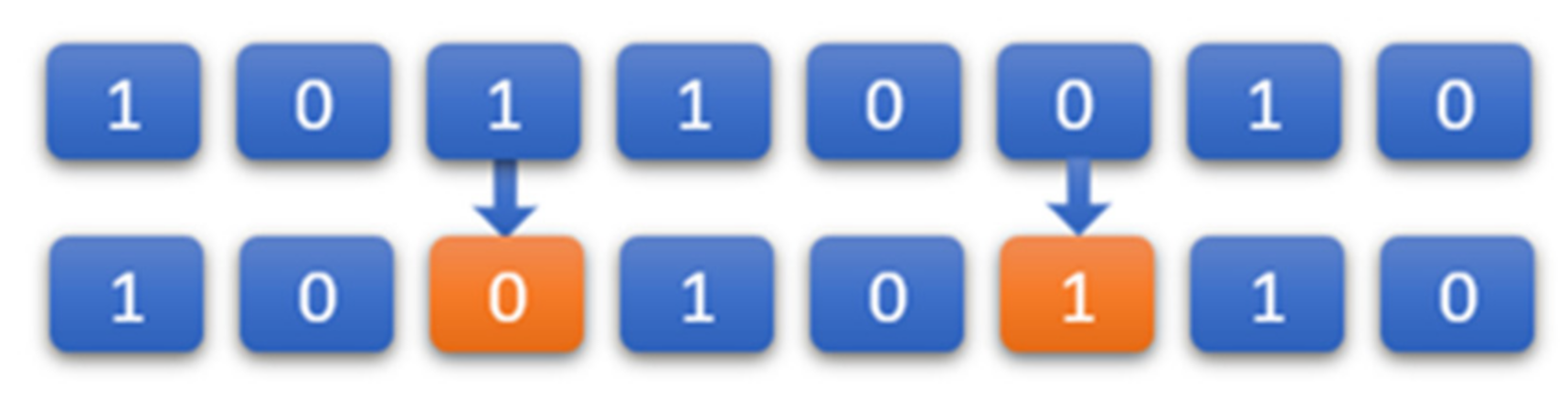
The EOA employs various search mechanisms including both exploratory and exploitative ones to randomly change the solutions. The search agents represent the particles with their concentrations, and the optimal results represent the equilibrium state. The concentrations are randomly updated, considering the best-so-far solutions, called equilibrium candidates. This random updating, along with an accurate generation rate value, enhances EOA’s exploratory behavior in the initial iterations and the exploitative search in the final iterations, avoiding the search being trapped in local optima. In addition, balancing exploration and exploitation provides an adaptive value for the control parameter, and thus will reduce the magnitude of the motions of the particles. EOA depends on G to move from exploration to exploitation and to select the current exploitation method. Additionally, G is used to avoid the particles becoming trapped in local optima. However, G might quickly change its convergence speed towards the optimal solution, which may cause the particles to fall to a local optimum problem. [21]. In this subsection, we explain the proposed three MSS that enhance both the global and local search in the EOA algorithm, and help avoid being stuck in local optima, to some extent.

3.3.1. Mutation

The mutation method is used in GA to improve the diversity of the chromosome population. The mutation factor is employed to avoid being trapped in local optima by creating a more innovative and evolutionary solution to the problem. There are many types of mutations that rely on the algorithm used and the designated problem. However, in this study we applied a bit chain mutation that functioned by twisting features at arbitrary positions. For example, assuming X = (x₁, x₂, …, x_D) is a location of the current particle’s, then the bit chain mutation can be mathematically formulated as in (18)

$$MU \left(i\right)=\left|1-X\left(i\right)\right|$$

(18)

where MU is the particle (solution) after utilizing bit chain mutation, I = 1, 2, …, D is an array of randomly selected positions that twisted in solution X. Figure 1 shows an example of solution X, where the third and sixth positions are twisted. Due to various empirical observations and error tests, the mutation rate is randomly selected between 10% and 25% in the exploration phase, and between 1% and 9% in the exploitation phase. EOA relies on the generation rate G to switch from exploration to exploitation search. The ratio of G controls the selection of the global search when it is greater than 0.5, and the exploitation phase when it is less than 0.5. Based on Equations (10) and (11), the value of G is based on G₀ and F, as in Equation (9). Therefore, in the first fifty percent of iterations, the G value is varied between [0, 2], and in the second fifty percent it is fluctuated between [0, 1]. Consequently, EOA can perform exploration and exploitation in the first part of the iterations. However, in the second part, it can only perform exploitation.

In IEOA, we included the G value to select the number of features to be twisted. Generally, in the global search, more features of the current best solution need to be twisted to improve the power of the exploration. However, in the local search, the particles are supposed to be closer to the equilibrium state (optimal solution). Therefore, fewer features are twisted to improve the exploitation. Thus, the mutation rate is mathematically formulated as in (19)

$$Mutatio{n}_{rate}=\left\{\begin{array}{ll}No of Featuers\ast \frac{10\ast rand\left[1,5\right]}{100}& if G\ge 1\\ No of Featuers\ast \frac{rand\left[1,9\right]}{100}& if G<1\end{array}\right.$$

(19)

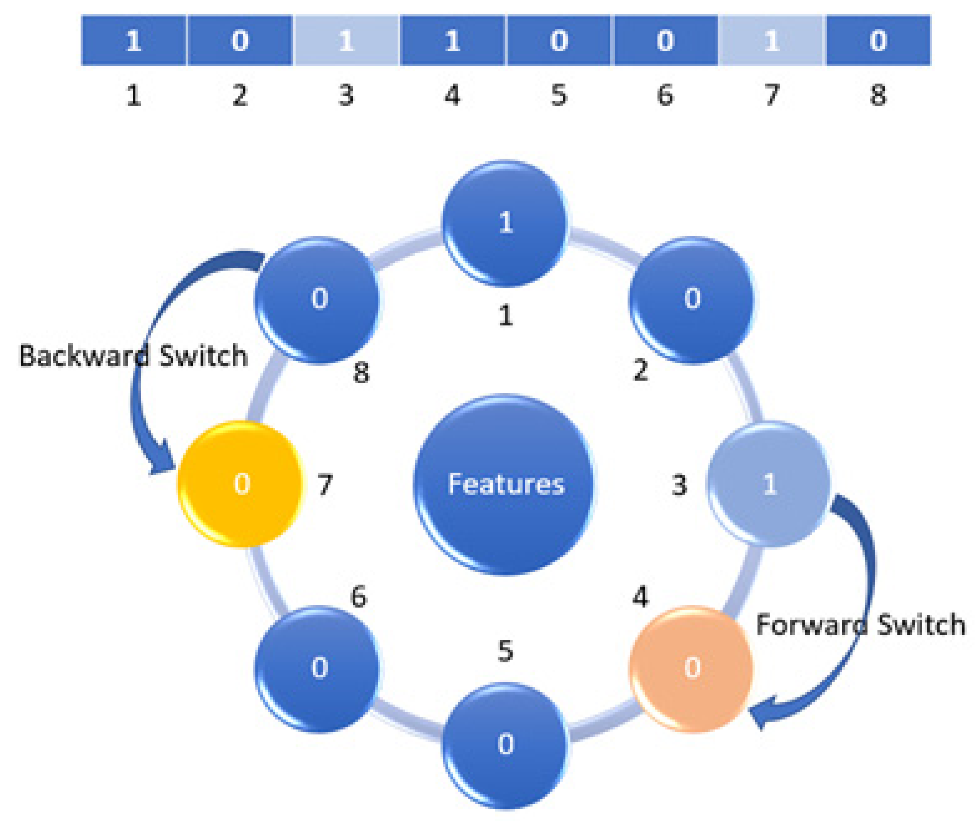
3.3.2. Mutation Neighborhood Method (MNM)

MNM was applied by Das et al. in 2009 [50] in order to balance between global and local search in differential evolution. The idea of the neighborhood search is to use the mutation operator to search a small region around the current best solution instead of searching the whole population. In this proposed work, we applied MNM. MNM search is monitored by the current best solution found by the mutation method. In other words, whenever a mutation causes a change in the position of the current best solution (equilibrium state), MNM will be applied. However, after the current best position is mutated, the fitness value will be calculated again in every iteration. If the fitness value of the new-found location is better than the current location, the current best solution is replaced with the new mutated solution, and thus the MNM search is performed.

Essentially, the MNM considers two contiguous techniques of the switched feature. First, in the forward switched technique, the right feature is mutated, and then fitness values for the two solutions (the best solution with the current switched solution) are evaluated. Second, in the backward switched technique, the same technique is applied but the left feature is mutated. Consequently, two solutions are created, and the best value is ranked as the best solution. Furthermore, the MNM circle is used, as the last feature is connected to the first feature to have two contiguous neighbors on both sides. Figure 2 explains the technique of the MNM circle.

3.3.3. Backup Method (BM)

Mutation is a powerful strategy that can effectively improve the exploration and exploitation process. However, it might change the direction of the optimization algorithm and lead to a local optimum. Generally, local optima are one of the common challenges for optimization algorithms. Therefore, BM is included in the proposed IEOA. BM is a straightforward and functional method. In BM, if the new mutated solution has a better fitness value than the current solution, it will not be immediately considered as the current best solution. It will be tentatively saved as a possible solution for the next iteration. If the EOA results at the next iteration achieved a better solution, the current best solution is also modified. Then, the possible solution (BM solution) is compared with the current best solution, and at this round the higher solution value is considered to be the best current best solution. However, MSS accepts the new location resulting from mutation or MSM if it maintains the best fitness value for two consecutive iterations.

4. Improved Equilibrium Optimization Algorithm (IEOA)

This section introduces IEOA, which is an improved version of EOA. The IEOA utilizes the powers of EOA and tunes it for the FS problem. Particularly, two main improvements for EOA were introduced. The first improvement involves employing the EOBL method at the initialization phase. This improvement enhances the diversity of the population. The second improvement involves employing enhanced MSS. This improvement strengthens the search abilities of the algorithm in both local and global search. In IEOA, the feature subset in the FS problem is considered a binary value consisting of “1” and “0”. The value of “1” indicates the corresponding feature is selected, while “0” indicates that the corresponding feature is not selected, as in Equation (13). The framework of the proposed IEOA using EOBL and MMS strategies is illustrated in Figure 3. The steps of the proposed IEOA algorithm are illustrated as follows:

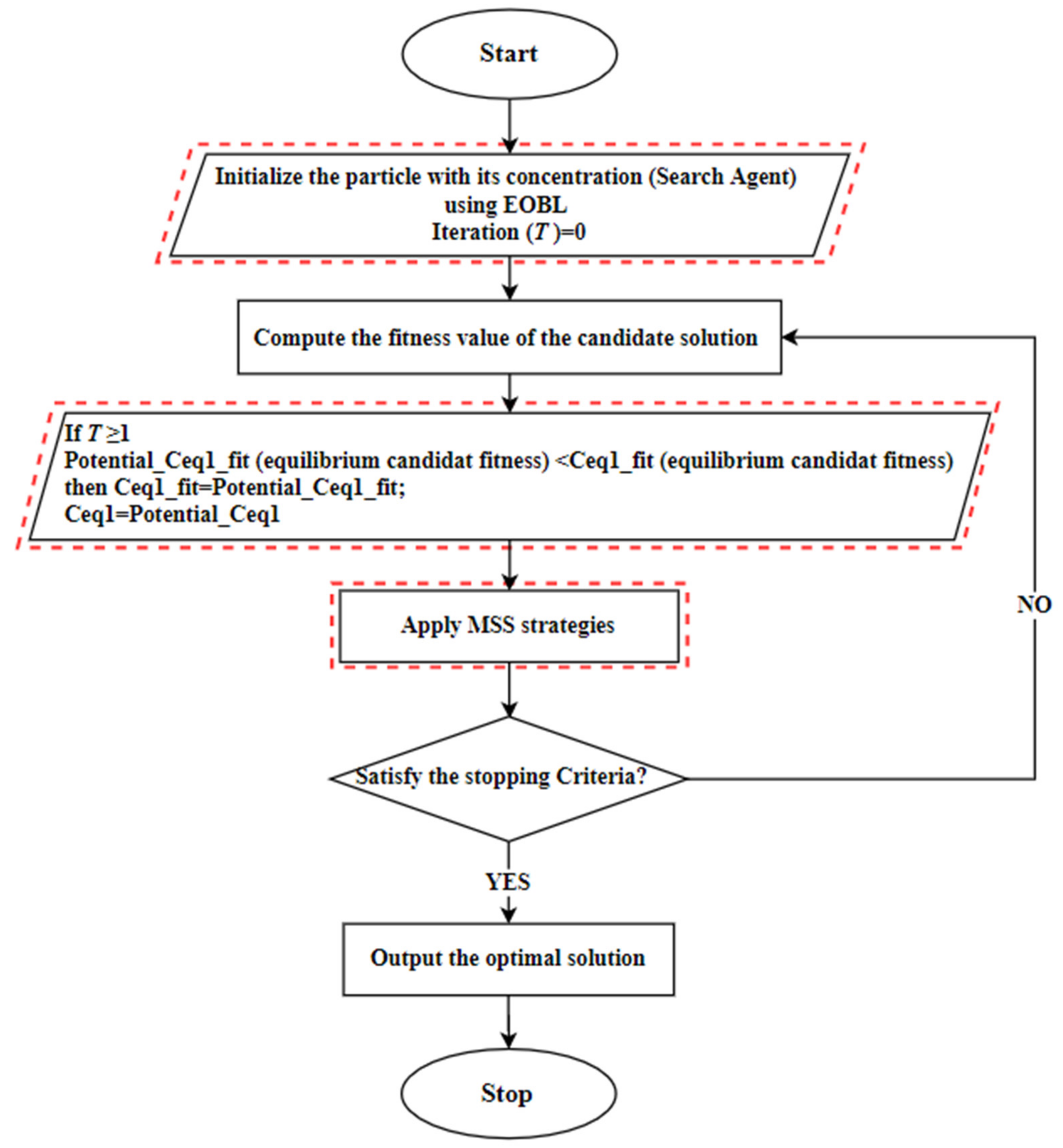
• In the first step: the particle population C is initialized using the random generation function with the size N, as defined in Equation (2) and the equilibrium candidate’s fitness is assigned with a large number. In this step, each generated particle (search-agent) is regarded as a possible solution, which includes a random set of features from the complete set of features.
• In the second step: compute the fitness value of each solution and find the elite position from the initial population. After that, the EOBL method creates the opposite elite solutions, as defined in Equation (15), then selects the best N solution.
• In the third step: the EOA algorithm is executed to update the location of each particle in the population and to find the best current location based on the best fitness value, as defined in Equation (13). IEOA works based on KNN classification accuracy and the feature selection is based on the wrapper mode.
• In the fourth step: MSS strategies are employed to improve the current location. Here, a potential best solution is considered; if the fitness value of a new location is better than the current one, then the MNM is executed for further improvement.
• The next iteration of EOA is executed and the current best solution compared with the potential solution in the fifth step. Here, the BM strategy is used if the current best solution is better than the potential location. Otherwise, the current best location is changed to be equal to the potential solution
• In the sixth step: The proposed solution proceeds with the iterations until the stopping criteria is met. The pseudocode of the proposed IEOA is illustrated in Algorithm 1.

Algorithm 1. Pseudo code of IEOA Algorithm.

Input: Initialize the particle’s population randomly$C_i \left(i=1,2,\dots ,N\right)$, T: the maximum number of iterations. Output: The equilibrium state and its fitness value. Apply EOBL method to find the best$N$opposite solutions, then select the fittest$N$solutions, according to Equations (14)–(16) Assign free parameters$a_1=2; a_2=1;GP=0.5;$ $\mathit{While} \left(Maximum iteration not reached \left(Iter<T\right)\right) \mathit{do}$ Calculate the fitness of the particle locations. $For i=1: number of particles \left(n\right)$  $If fit\left(C_i\right)<fit\left(C_{eq1}\right)$   $Replace C_{eq1} with C_i and fit \left(C_{eq1}\right) with fit \left(C_i\right)$  $Elseif fit\left(C_i\right)>fit\left(C_{eq1}\right) \& fit\left(C_i\right)<fit\left(C_{eq2}\right)$   $Replace C_{eq2} with C_i and fit \left(C_{eq2}\right) with fit\left(C_i\right)$  $Elseif fit\left(C_i\right)>fit\left(C_{eq1}\right) \& fit\left(C_i\right)>fit\left(C_{eq2}\right) \& fit\left(C_i\right)<fit\left(C_{eq3}\right)$   $Replace C_{eq3} with C_i and fit\left(C_{eq3}\right) with fit\left(C_i\right)$     $$\begin{gathered} Elseif fit\left(C_i\right)>fit\left(C_{eq1}\right) \& fit\left(C_i\right)>fit\left(C_{eq2}\right) \& fit\left(C_i\right)>fit\left(C_{eq3}\right) \& fit\left(C_i\right) \\ \hspace{1em}\hspace{1em}\hspace{1em}<fit\left(C_{eq4}\right) \end{gathered}$$   $Replace C_{eq4} with C_{i}and fit \left(C_{eq4}\right) with fit \left(C_i\right)$  $End\left(If\right)$ $End\left(For\right)$ $C_{ave}=\frac{C_{eq1}+C_{eq2}+C_{eq3}+C_{eq4}}{4} \hspace{1em}\hspace{1em}\hspace{1em}\hspace{1em}\hspace{1em}\hspace{1em}from Equation \left(3\right)$ $C_{eq.pool}=\left\{C_{eq\left(1\right) },C_{eq\left(2\right) },C_{eq\left(3\right) }, C_{eq\left(4\right) },C_{eq\left(ave\right)}\right\} \hspace{1em}\hspace{1em}\hspace{1em}from Equation \left(4\right)$ $Assign t={\left(1-\frac{Iter}{T}\right)}^{(a_2\frac{Iter}{T})} \hspace{1em}\hspace{1em}from Equation \left(6\right)$ $For i=1:number of particles \left(n\right)$ $Constract F=a_1\sin \left(r-0.5\right)\left[e^{-\lambda t}-1\right] \hspace{1em}\hspace{1em}from Equation \left(8\right)$ $Constract G=G_0.F \hspace{1em}from Equation \left(9\right)$ $Constract G_0=GCP \left(C_{eq}-\lambda C\right) \hspace{1em}from Equqtion \left(10\right)$ $Constract GCP=\left\{\begin{array}{c}{0.5}_{r1} r_2\ge GP \\ 0 r_2<GP \hspace{1em}\hspace{1em}\hspace{1em}\hspace{1em}\end{array}\right.from Equation \left(11\right)$ $C=C_{eq}+\left(C-C_{eq}\right) . F+\frac{G}{\lambda V} \left(1-F\right) \hspace{1em}from Equation \left(16\right)$ $End\left(For\right)$ $For \left(i=1 to 8\right) do$%MSS        $If (fitness C_{potential}<fitness C_{Best sloution \left(Iter+1\right)}$ $then=C_{Best solution}=C_{potential}$ $Else C_{Best solution}=C_{Best solution \left(iter+1\right)}$%BM Apply mutation strategy to current best location$C_{Best solution}$ using Equations (17) and (18)        $If current location \left(C_{mutation}<C_{Best solution} \right)$ $then Apply \mathit{MNM} search on C_{mutation}$ $Set C_{potential}=C_{mutation}$ Return the best location$\left(C_{Best solution}\right)$ $Iteration=Iter+1$ $End While$

5. Experiments

5.1. Platform

The performance of IEOA was evaluated and compared with the original EOA and some popular and new optimization algorithms, including the GOA, GA, PSO, ALO, WOA, BOA, and SMA algorithms. All the experiments were executed using MATLAB R2020b 9.9 (Natick, MA, USA), and operated on a PC running with an Intel Core i7-8550U, 1.80 GHz, 16 GB of RAM, and Windows 10 version 20H2 operating system.

The displayed Equations (20)–(23) are the computation methods of the average value classification accuracy, the average fitness value, and the average of the selected feature, respectively.

$$Avg\_acc=\frac{1}{30}{\displaystyle \sum }_{i=1}^{30}ac{c}_i$$

(20)

Avg_acc is the average classification accuracy scored by running the algorithm independently for 30 iterations, acc_i symbolizes the classification accuracy scored from each iteration. acc_i is computed as in (21)

$$ac{c}_i=\frac{1}{N}{\displaystyle \sum }_{c=1}^{N}match\left(C{L}_c , A{L}_c\right)$$

(21)

where N symbolizes the total number of test cases. CL_c is the class label of the expected class data, AL_c is the existing class in the labeled data. In addition, match(CL_c, AL_c) is a discrimination function. When CL_c and AL_c are equal, match(CL_c, AL_c) = 1, if not match(CL_c, AL_c) = 0.

$$Avg\_fitness=\frac{1}{30}{\displaystyle \sum }_{i=1}^{30}fitnes{s}_i$$

(22)

Avg_fitness is the average fitness value acquired by running the algorithm for 30 iterations, and fitness_i represents the best fitness value acquired from each run.

$$Avg\_feature=\frac{1}{30}{\displaystyle \sum }_{i=1}^{30}featur{e}_i$$

(23)

where Avg_feature is the average value of the selected feature acquired by running the algorithm for 30 iterations, and f_i is the value of the selected number of features acquired from each run.

5.2. Benchmark Datasets

To validate the efficiency of the proposed IEOA algorithm, the experiments were conducted on 21 benchmark medical datasets from the UCI repository. The selected datasets were utilized to determine the capabilities of the IEOA algorithm. In addition, to confirming the solidity of IEOA, two feature dimensionalities were used, including average and high dimensionality. The selected datasets have been used in many feature selection problems, such as [37,51,52].

Table 1. UCI Medical Datasets Details.

Dataset	Features	Sample	Dimensionality
Primry_Tumer	17	339	Average
Hepatitis	20	155	Average
Lymphography	19	148	Average
Breast_Cancer	10	699	Average
Echocardiogram	12	132	Average
Fertility	10	100	Average
Leaf	16	340	Average
Lung_Cancer	57	32	Average
Diabetic	20	1151	Average
ILPD	11	583	Average
Cortex_Nuclear	82	1080	High
Epileptic_Seizure	179	11,500	High
Promoter-gene	58	116	High
WDBC	31	569	High
Cervical cancer	36	858	High
Arrhythmia	279	452	High
Dermatology	35	366	High
Heart Disease	75	303	High
HCV	29	1385	High
Parkinson	29	1040	High
HCC	50	165	High

presents the details of the selected datasets.

5.3. Algorithms and Experiment Parameter Setting

In this work, the parameters were set after many experimental observations and similarly to [32]. Additionally, it has been noted that adjusting the control parameter can improve the performance of the algorithm. Therefore, the random parameter settings are very important and should be chosen carefully. In this experiment, the K-nearest-neighbors (KNN) classifier (wrapper mode) with 10-fold cross-validation was used to evaluate the performance of the algorithms. The validation of the dataset was divided into ten equal parts (fold). Nine-folds were used in the training phase, and the final fold was used for the testing.

Furthermore, in order to ensure the fairness of the comparison, the maximum number of iterations of each algorithm was set to 50 iterations. Moreover, the experiments were repeated 30 times and considering the settings used in [12,37]. Therefore, the results were obtained from an average of 30 runs. The parameter settings for the proposed IEOA are presented in

Table 2. IEOA Parameter Setting.

Parameter	Value
Population size	10
Number of iterations	50
Dimension	Number of Feature
Number of runs for each method	30
α	0.99
β	0.01

. In addition, the general parameter settings for the baseline algorithms are displayed in

Table 3. Parameter Settings of Optimization Algorithms.

Algorithm	Parameters	Reference
PSO	Inertia Weight value 0.9 Inertia Weight Damping Ratio 0.4 Accelerating-constant values are C1 = 2, C2 = 2	[53]
GA	Crossover Ratio 0.9 Mutation Rate 0.2	[54]
WOA	A [2, 0]	[21]
GOA	cMax = 1 cMin = 0.00004	[26]
ALO	K = 500	[55]
SMA	z = 0.03	[56]
BOA	Probability-switch 0.8 Power exponent = 0.1 Sensory modality = 0.01	[57]

.

5.4. Computational Complexity

The computational complexity of IEOA relies on the number of particles (N), the number of dimensions (D), the number of iterations (T), and the cost of function evaluation and MSS solution (C). This complexity is modelled by a function that relates the running time of the algorithm to the input size of the problem. Accordingly, Big –O-Notation is used here as a popular term, as in (24)

$$\begin{array}{c}O \left(EOA\right)=O\left(Problem definition\right)+O\left(Initilization\right)\hfill \\ \hspace{1em}\hspace{1em}\hspace{1em}\hspace{1em}\hspace{1em}\hspace{1em}\hspace{1em}\hspace{1em}\hspace{1em}\hspace{1em}\hspace{1em}\hspace{1em} +O\left(t\left(function evaluation\right) \right)+O\left(t\left(Memory saving\right)\right)\hfill \\ \hspace{1em}\hspace{1em}\hspace{1em}\hspace{1em}+O\left(t\left(Concentration update\right)\right)\hfill \end{array}$$

(24)

Moreover, the computational complexity of utilizing the MSS strategy can be computed as O(T*I*M), where I is the number of MSS iterations, and M is the MSS search strategies, together with mutation and MNM. Consequently, the computational complexity of IEOA is presented in (25)

$$O\left(IEOA\right)=O\left(1+ND+TCN+TN+TND+TIM\right)\cong O\left(TND+TCN\right)$$

(25)

6. Results and Analysis

This section demonstrates the effectiveness of the proposed IEOA by performing two main experiments. The first experiment included the comparison of the proposed IEOA with the standard EOA. The second experiment involved the comparison of IEOA with state-of-the-art algorithms, such as GOA, GA, PSO, ALO, WOA, BOA, and SMA. In all conducted experiments, each algorithm was utilized on all the datasets to verify the solidity of the algorithm within feature dimensionalities. Additionally, the reported results are based on computing the average of 30 runs for every experiment.

6.1. Comparison of EOA and IEOA

This section includes the proposed IEOA in comparison with the original EOA. The comparison is based on four metrics, which are the average classification accuracy, the average number of selected features, average fitness value, and p-value (Wilcoxon test) as a statistical test.

Table 4. The Experimental Results of the IEOA in Comparison to the Original EOA in Terms of Classification Accuracy, Number of Selected Features, and Fitness value and p-value, the best results are underlined.

Dataset	Classification Accuracy		Selected Feature		Fitness		EOA p-Value
	EOA	IEOA	EOA	IEOA	EOA	IEOA
Primry_Tumer	0.85556	0.88604	6.3667	6.8667	0.14675	0.11686	0.0398
Hepatitis	0.86319	0.89514	3.3	3.1	0.13717	0.10587	0.00203
Lymphography	0.74192	0.79155	6.8333	5.0333	0.25874	0.20972	0.0624
Breast_Cancer	0.98476	0.98714	3.3	3.1667	0.018308	0.016247	0.296
Echocardiogram	0.90586	0.9185	1.9	1.1	0.028925	0.016475	0.0474
Fertility	0.72333	0.74667	1.7667	2.1	0.077863	0.055133	0.0541
Leaf	0.78373	0.81634	5.1333	5.1333	0.21753	0.18558	0.0112
Lung_Cancer	0.53611	0.55833	1.4	1.1	0.0305	0.008446	0.0384
Diabetic	0.99697	0.99697	7.1	5.5333	0.004268	0.003988	0.146
ILPD	0.55061	0.55119	25	26.7333	0.4463	0.44605	0.912
Cortex_Nuclear	0.98152	1	6.8	6.4667	0.019493	0.001135	0.0189
Epileptic_Seizure	0.96895	0.97539	3.1333	3.0333	0.03178	0.025379	0.0966
Promoter-gene	0.97475	0.98096	2.9333	2.9333	0.022737	0.017753	0.27
WDBC	0.99635	1	8.4333	6.9667	0.006098	0.002966	0.00898
Cervical cancer	0.90494	0.91975	3.4667	3.5	0.096778	0.082137	0.357
Arrhythmia	0.34425	0.35914	4.4333	4.4	0.65086	0.63621	0.0211
Dermatology	1	1	1.0333	1	0.000369	0.000357	0.334
Heart Disease	0.76492	0.78154	54	54.9333	0.23467	0.21861	0.0252
HCV	0.7482	0.77193	5.1333	5.0333	0.25199	0.24217	0.00302
Parkinson	0.78403	0.80118	2.9333	3.1333	0.21674	0.19997	0.0684
HCC	0.8826	0.90882	5	3.8667	0.11725	0.091054	0.0771

demonstrates the experimental results of the IEOA in comparison with the original EOA, the best results are underlined. For the statistical tests, if the p-value was lower than 0.05, then the improvement was considered to be significant; otherwise, it was not significant. The p-value was utilized to determine if the classification accuracy of IEOA improved significantly.

According to the results, IEOA outperformed EOA for the majority of the datasets in terms of classification accuracy, while it provided similar accuracy to EOA in two datasets. Consequently, it is obvious that the use of EOBL and MSS improve the performance of IEOA. In terms of the number of selected features, IEOA outperformed the standard EOA by decreasing the number of selected features in 15 datasets, while it was comparable with EOA in two datasets, and EOA was better in six datasets. In terms of fitness value, IEOA outperformed EOA in all datasets. Statistically, the p-value shows that the IEOA significantly outperformed EOA in 15 datasets. Therefore, IEOA significantly improved the classification accuracy, feature selection, and fitness value across the different dataset’s dimensions.

In addition, it can be observed from the stated results in Table 4, that the use of EOBL, achieved using Equation (15), improved the choice of solutions, instead of using the random methods in the original EOA. The possible reason is that the EOBL chose the best obtainable solutions. Thus, compared with solutions produced by random methods, there are fewer opportunities to choose weak solutions. Furthermore, the use of the MSS method improves the algorithm’s capabilities in balancing exploration and exploitation. The algorithm uses the current best location to update the positions of the other search agents. Therefore, the use of the proposed MSS enhanced the algorithm’s exploration capability when looking for promising areas. Moreover, by using the mutation methods in Equations (18) and (19), the algorithm avoided dropping into a local solution. Furthermore, both the proposed mutation method and the MNM search increased the algorithm’s exploitation capability, searching for the best solution in a specified local area. Consequently, the superiority of IEOA was demonstrated in three main aspects: the number of selected features, the classification accuracy, and the fitness value.

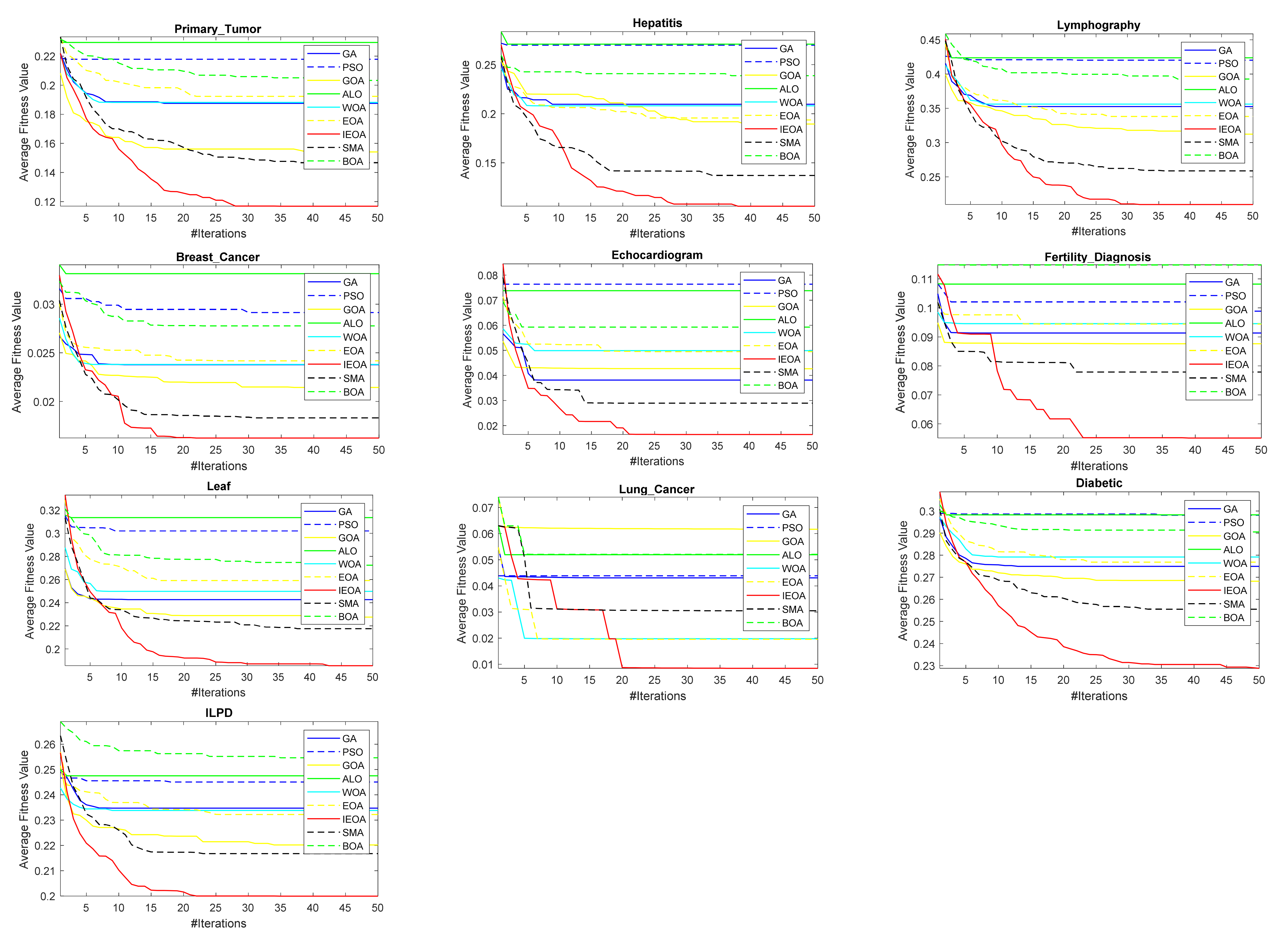
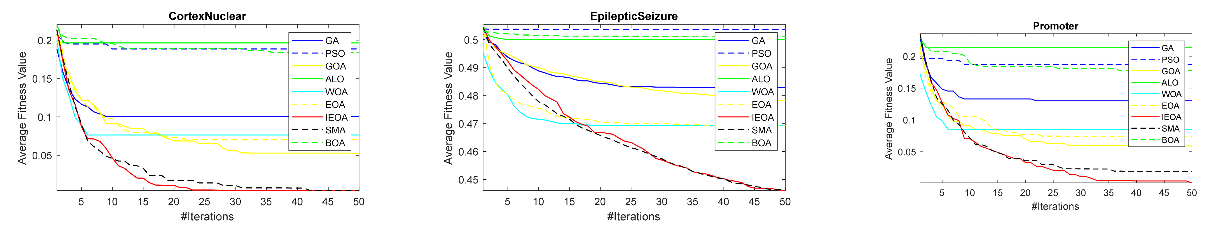
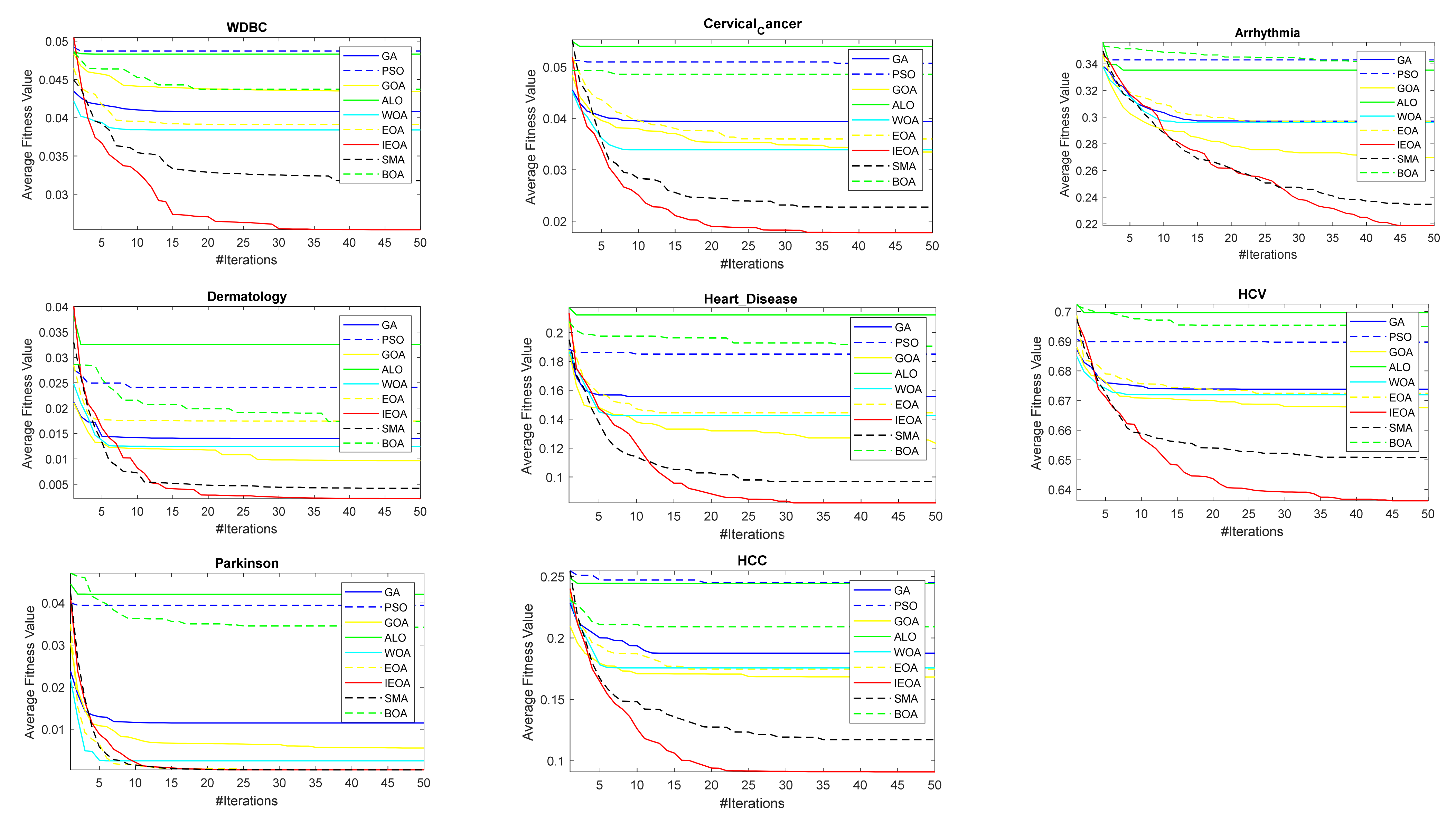
6.2. Comparison of IEOA Algorithm with Other Optimization Algorithms

The previous experiments proved the superiority of IEOA, especially in terms of classification accuracy and fitness value over the original EOA. This superiority is a result of improving the population diversity and achieving an appropriate balance between exploration and exploitation for preventing the local optima. Therefore, to validate the advantage of IEOA, an additional comparison was made between IEOA and highly citied and recent optimization algorithms like GOA, GA, PSO, ALO, WOA, BOA, and SMA. Here, we also used the four-evaluation indicators to evaluate the performance of IEOA compared with the other optimization algorithms. First, the classification accuracy was evaluated for the considered algorithms, as in

Table 5. The Classification Accuracy of IEOA and Other Optimization Algorithms.

Dataset	IEOA	GOA	GA	PSO	ALO	WOA	BOA	SMA
Primry_Tumer	0.88604	0.77302	0.8153	0.84878	0.81438	0.80945	0.78586	0.80059
Hepatitis	0.89514	0.73056	0.79181	0.81153	0.79222	0.80694	0.73264	0.76389
Lymphography	0.79155	0.57721	0.64861	0.68843	0.64447	0.66259	0.58146	0.60909
Breast_Cancer	0.98714	0.97143	0.98048	0.98238	0.98	0.98	0.97667	0.97667
Echocardiogram	0.9185	0.86282	0.89799	0.89267	0.88535	0.88516	0.86007	0.87766
Fertility	0.74667	0.69333	0.71	0.71333	0.70667	0.70667	0.70333	0.68667
Leaf	0.81634	0.68839	0.75952	0.7742	0.75276	0.7432	0.70144	0.7314
Lung_Cancer	0.55833	0.51667	0.525	0.50556	0.54722	0.54722	0.525	0.51667
Diabetic	0.99697	0.80606	0.90273	0.95	0.92485	0.93091	0.81515	0.81939
ILPD	0.55119	0.49977	0.51701	0.52188	0.52762	0.52696	0.49661	0.49919
Cortex_Nuclear	1	0.78848	0.87333	0.94364	0.91576	0.92667	0.81667	0.82606
Epileptic_Seizure	0.97539	0.95547	0.96192	0.95841	0.96426	0.9625	0.95605	0.95547
Promoter-gene	0.98096	0.9162	0.93019	0.93523	0.93406	0.93172	0.9201	0.92204
WDBC	1	0.96189	0.98448	0.99094	0.99089	0.98549	0.98181	0.98358
Cervical cancer	0.91975	0.79012	0.84691	0.87901	0.85926	0.85679	0.81852	0.81235
Arrhythmia	0.35914	0.29806	0.32258	0.32837	0.32376	0.32355	0.30884	0.30309
Dermatology	1	0.96218	0.99167	0.99647	0.9984	1	0.96538	0.97083
Heart Disease	0.78154	0.66622	0.70459	0.73192	0.70461	0.70283	0.65969	0.66047
HCV	0.77193	0.67662	0.71719	0.72008	0.70907	0.7053	0.68271	0.69169
Parkinson	0.80118	0.75471	0.76685	0.78117	0.7674	0.76858	0.75761	0.7479
HCC	0.90882	0.75784	0.81409	0.83284	0.82426	0.82488	0.75784	0.79387
Mean value (F-test)	0.840313	0.745098	0.783917	0.799373	0.788918	0.789877	0.752545	0.759456
Overall ranking	1	8	5	2	4	3	7	6

. According to the results obtained, IEOA outperformed the other algorithms for the selected datasets in terms of classification accuracy, the significant results are underlined, whereas it gave a similar accuracy to WOA in one dataset. The average accuracy of IEOA was 9.52% higher than GOA, 8.8% than BOA, 8.1% than SMA, 5.64% than GA, 5.14% than ALO, 5.04% than WOA, and 4.1% than PSO. The classification accuracy results for IEOA and all algorithms are displayed in Table 5. The Wilcoxon test was applied to verify the significance of classification accuracy, as displayed in

Table 6. p-Values for The Classification Accuracy Based on Wilcoxon Test.

Dataset	GOA	GA	PSO	ALO	WOA	BOA	SMA
Primry_Tumer	4.64 × 10−8	4.92 × 10−5	3.92 × 10−3	1.01 × 10−5	1.80 × 10−5	8.41 × 10−9	3.51 × 10−5
Hepatitis	8.84 × 10−10	9.49 × 10−7	2.58 × 10−5	1.98 × 10−6	3.35 × 10−5	3.80 × 10−10	1.30 × 10−6
Lymphography	5.99 × 10−8	2.06 × 10−5	1.76 × 10−3	9.50 × 10−6	1.17 × 10−4	9.24 × 10−9	2.84 × 10−5
Breast_Cancer	5.29 × 10−6	1.71 × 10−2	6.59 × 10−2	2.18 × 10−2	2.01 × 10−2	3.41 × 10−4	5.00 × 10−2
Echocardiogram	2.85 × 10−6	1.77 × 10−3	3.83 × 10−3	1.77 × 10−3	1.02 × 10−2	2.10 × 10−6	3.62 × 10−3
Fertility	5.51 × 10−2	1.42 × 10−1	4.34 × 10−1	2.19 × 10−1	2.21 × 10−1	4.89 × 10−2	8.41 × 10−2
Leaf	3.00 × 10−7	1.40 × 10−3	2.65 × 10−2	1.14 × 10−3	3.27 × 10−4	6.73 × 10−6	5.59 × 10−3
Lung_Cancer	4.30 × 10−2	4.30 × 10−2	4.14 × 10−2	4.51 × 10−1	8.58 × 10−1	4.30 × 10−2	8.77 × 10−2
Diabetic	3.18 × 10−11	5.79 × 10−11	3.47 × 10−10	1.80 × 10−5	2.36 × 10−5	3.52 × 10−11	6.36 × 10−10
ILPD	4.07 × 10−11	2.67 × 10−9	8.88 × 10−10	4.44 × 10−7	1.36 × 10−7	3.02 × 10−11	5.59 × 10−9
Cortex_Nuclear	2.88 × 10−11	2.88 × 10−11	4.28 × 10−11	1.62 × 10−6	9.40 × 10−7	2.89 × 10−11	5.30 × 10−11
Epileptic_Seizure	4.61 × 10−7	7.50 × 10−6	3.69 × 10−6	1.72 × 10−4	8.14 × 10−4	9.90 × 10−7	2.74 × 10−6
Promoter-gene	1.91 × 10−8	1.10 × 10−6	3.45 × 10−5	2.03 × 10−5	6.04 × 10−5	5.65 × 10−9	6.10 × 10−6
WDBC	5.95 × 10−11	2.00 × 10−10	8.41 × 10−9	1.90 × 10−9	7.90 × 10−10	1.08 × 10−10	2.74 × 10−10
Cervical cancer	1.09 × 10−10	2.47 × 10−7	1.16 × 10−3	4.21 × 10−5	1.05 × 10−5	1.21 × 10−8	7.34 × 10−7
Arrhythmia	8.95 × 10−11	2.77 × 10−7	2.68 × 10−5	2.02 × 10−7	2.28 × 10−7	2.19 × 10−7	7.96 × 10−7
Dermatology	1.21 × 10−12	1.19 × 10−12	4.36 × 10−12	3.06 × 10−4	2.15 × 10−2	1.21 × 10−12	5.35 × 10−11
Heart Disease	9.83 × 10−8	7.20 × 10−5	5.08 × 10−3	3.83 × 10−5	2.13 × 10−4	9.06 × 10−8	9.53 × 10−5
HCV	3.45 × 10−10	4.42 × 10−7	1.38 × 10−5	2.10 × 10−7	8.81 × 10−7	2.15 × 10−10	2.06 × 10−7
Parkinson	2.93 × 10−5	7.04 × 10−4	2.49 × 10−2	7.43E × 10−4	9.42 × 10−3	2.75 × 10−5	4.03 × 10−4
HCC	6.65 × 10−10	2.55 × 10−7	1.63 × 10−5	9.74 × 10−6	3.06 × 10−6	2.58 × 10−10	1.21 × 10−7

, the best results are underlined. Accordingly, the significant results were verified, with a p-value < 0.05, for all algorithms and datasets except GA, PSO, and ALO. There was no significance in only one dataset, which was Fertility. Therefore, these significant results proved the superiority of IEOA over all the other algorithms. The results signify the capability of IEOA to balance exploration and exploitation. Moreover, it has a better chance of avoiding the trap of local optima, which ultimately led to a significant improvement in the classification accuracy of IEOA.

The average number of the selected features is displayed in

Table 7. The Average Number of Selected Features for IEOA and Other Optimization Algorithms.

Dataset	IEOA	GOA	GA	PSO	ALO	WOA	BOA	SMA
Primry_Tumer	6.3667	7.9	7.9667	7.4667	7.5	6.2667	9.9333	10.0333
Hepatitis	3.3	7.9333	6.7333	5.6333	4.4	4.7333	9.7333	9.5
Lymphography	6.8333	9.1333	8.3333	6.8667	7.5333	7.4	10.4333	10.3667
Breast_Cancer	3.3	4.3667	4	3.6	3.6	3.9333	5.4333	4.2
Echocardiogram	1.9	4.3667	3.4667	2.6667	2.6	2	4.2667	4.6
Fertility	1.7667	2.3333	2.0333	1.6667	1.9667	1.8333	2.8667	2.3667
Leaf	5.1333	7.5333	6.8	5.9667	7.6333	7.3	9.7	9.8
Lung_Cancer	1.4	13.6	10.1	6.7333	3.1	1.7333	14.7333	14.3667
Diabetic	7.1	24.8333	23.8333	17.9667	10.9	10.7333	31.3	27.1667
ILPD	25	86.5667	84	86.7333	28.7	20.1	94.4	92.1333
Cortex_Nuclear	6.8	26.7333	25.4	19.1667	10.8	10.3	33.1	30.9333
Epileptic_Seizure	3.1333	12.7	9.2667	6.7	9.1	5.9667	15.6	14.5333
Promoter-gene	2.9333	14.1	11.4	8.0667	5.6667	4.9333	16.1333	15.3667
WDBC	8.4333	16.9667	15.0667	11.4667	15.5333	14.3333	21.2	18.8667
Cervical cancer	3.4667	5.7	5.2	4.4667	4.1	3.4	6.9333	6.1333
Arrhythmia	4.4333	13.3	9	7.5333	6.9333	7.8	15.3	14.2
Dermatology	1.0333	12.9667	9.1333	5.7333	2.5333	1.3667	14.5333	15.0333
Heart Disease	54	133.5333	128.5	116.0333	100.1667	76.7667	167.2	153.5
HCV	5.1333	9.5333	7.6333	6.9667	8.3	7	11.5	9.9667
Parkinson	2.9333	4.6667	3.9	3.5333	3.5333	3.1	5.0667	5.0333
HCC	5	22.7667	17.3	13.5333	8.1667	6.0333	27.0667	24.7667
Mean value (F-test)	7.590467	21.0254	19.00317	16.59524	12.0365	9.858724	25.06825	23.46984
Overall ranking	1	6	5	4	3	2	8	7

for all algorithms for 30 runs, the best results are underlined. It can be observed that IEOA outperformed all the algorithms in terms of selected features. Moreover, IEOA ranked first by selecting fewer features in 21 datasets, the average of IEOA’s selected features was 7.5, followed by WOA with 9.85, then ALO with 12.03, then PSO with 16.59, and then GA with 19.003. GOA, SMA, and BOA gave a lower performance for the selected features, respectively. These results validate EOBL and MSM’s effectiveness for decreasing the number of selected features and increasing the classification accuracy. In addition, IEOA concentrates on promising regions in the search space to select the critical features and prevent irrelevant features.

Table 8. The Average of Fitness Function for IEOA and Other Optimization Algorithms.

Dataset	IEOA	GOA	GA	PSO	ALO	WOA	BOA	SMA
Primry_Tumer	0.11686	0.22935	0.18754	0.1541	0.18818	0.19233	0.21784	0.20331
Hepatitis	0.10587	0.27093	0.20966	0.18955	0.20802	0.19362	0.26981	0.23875
Lymphography	0.20972	0.42363	0.35251	0.31227	0.35616	0.33815	0.42015	0.39276
Breast_Cancer	0.016247	0.033138	0.023773	0.021443	0.0238	0.02417	0.029137	0.027767
Echocardiogram	0.016475	0.073777	0.038146	0.042677	0.049869	0.049505	0.076406	0.059303
Fertility	0.055133	0.10819	0.091359	0.087652	0.094585	0.094437	0.098885	0.11483
Leaf	0.18558	0.31352	0.24261	0.22752	0.24986	0.2591	0.30204	0.27245
Lung_Cancer	0.008446	0.051929	0.043054	0.061702	0.019804	0.01956	0.043881	0.052065
Diabetic	0.003988	0.19643	0.10056	0.052708	0.076346	0.070317	0.18859	0.18365
ILPD	0.44605	0.50009	0.48287	0.47821	0.46927	0.46944	0.50366	0.50098
Cortex_Nuclear	0.001135	0.21409	0.12986	0.059163	0.085295	0.074407	0.18731	0.17763
Epileptic_Seizure	0.025379	0.048316	0.040793	0.043411	0.038411	0.039114	0.048714	0.043717
Promoter-gene	0.017753	0.053989	0.039372	0.033431	0.033897	0.036003	0.05071	0.048573
WDBC	0.002966	0.042722	0.019792	0.012341	0.013587	0.018585	0.024247	0.021801
Cervical cancer	0.082137	0.21216	0.15556	0.12321	0.14249	0.14439	0.185	0.1905
Arrhythmia	0.63621	0.69967	0.67386	0.66761	0.67196	0.67247	0.68971	0.69501
Dermatology	0.000357	0.042073	0.011512	0.005538	0.002491	0.000488	0.03946	0.034244
Heart Disease	0.21861	0.33523	0.29706	0.26956	0.29603	0.29695	0.3429	0.34164
HCV	0.24217	0.32516	0.284	0.28079	0.29239	0.29543	0.32017	0.31047
Parkinson	0.19997	0.2475	0.23472	0.22017	0.23381	0.23221	0.24504	0.25462
HCC	0.091054	0.24438	0.18758	0.16825	0.17564	0.1746	0.24526	0.20912
Mean value (F-test)	0.12772	0.222204	0.183152	0.167205	0.177233	0.175966	0.215663	0.208247
Overall ranking	1	8	5	2	4	3	7	6

illustrates a comparison between IEOA and all optimization algorithms in terms of the average fitness value. The results show the superiority of IEOA, as the IEOA outperformed all the other algorithms in all datasets. The superiority in fitness values shows the reliable capabilities of IEOA.

Furthermore, applying the MSS methods accelerates the searching of a promising region and the best solution. Moreover, as can be noticed from Table 5 and Table 6, the datasets have a plurality of local optima, which implies a challenge to all optimization algorithms. Therefore, the ability of an algorithm to balance exploration and development can be distinguished. For example, the classification accuracy of the “Cortex_Nuclear” dataset displayed different results among the algorithms. The best accuracy “underlined” was accomplished by IEOA with 99%, followed by PSO with a 95% accuracy value, WOA with 93%, ALO with 92%, then with GA 90%, SMA and BOA gave a similar accuracy with 81%, and lastly, GOA with an 80% accuracy value. The proposed IEOA is an adaptable algorithm that searches for new promising areas, which is achieved by using the mutations method in Equation (18). This method prevents the algorithm from dropping into a local optima state.

Furthermore, the MNM strategy improved the local search of the IEOA by mining the promising area and exploring for a superior solution. Figure 4 and Figure 5 display graphical representations of the convergence curves. The convergences curves also need to be considered to evaluate the convergence speed of IEOA and the other optimization algorithms. In cases where the optimization algorithm cannot balance the exploration and exploitation in all iterations, it likely to converge to the local optimum. It can be observed from the convergence-curve results that IEOA accomplished a superior speed to all other algorithms, which implies the superiority of IEOA in processing different dimension datasets. Moreover, the effectiveness of the proposed MSS search strategies was notable, switching from exploration to exploitation search in the midpoint of iterations (from iteration 25 to the maximum iteration 50), and increasing the convergence speed in all cases. A brief comparison of IEOA with the other algorithms by calculating the average classification accuracy, selected features, and fitness value for all experiments is shown in

Table 9. Brief comparison of IEOA with all algorithms based on the average accuracy, features, and fitness.

Algorithms	Accuracy	Features	Fitness
EOA	1.69%	0.203%	1.59%
GOA	9.52%	13.43%	9.45%
GA	5.64%	11.41%	5.54%
PSO	4.09%	9.003%	3.95%
ALO	5.14%	4.44%	4.95%
WOA	5.04%	2.26%	4.82%
BOA	8.78%	17.47%	8.79%
SMA	8.09%	15.87%	8.05%
Average	6.00%	9.26%	5.89%

.

6.3. Limitations of the Proposed IEOA

Our proposed algorithm, IEOA, can solve high-dimensional and complex optimization problems. It has an edge over the original EOA, and this includes improving the classification accuracy and fitness value, and reducing the number of selected features. However, similarly to other optimization algorithms, IEOA has some limitations. The main limitation is the comparatively high-time consumption in comparison with the other algorithms. Nonetheless, the high-time consumption originated from the original EOA, and the proposed improvements had a marginal impact on the computational complexity of IEOA. An additional limitation is associated with the number of iterations in the proposed MSS. As such, we believe that the time complexity of IEOA can be reduced by replacing ten iterations of MSS with a less complicated solution.

7. Conclusions and Future Work

The equilibrium optimization algorithm (EOA) is a novel population-based optimization algorithm. EOA was inspired by the physics-based equation of mass balance. This study introduces an improved version of EOA, named IEOA, which adds two main improvements to the original EOA: (1) applying the EOBL method, and (2) employing MMS search strategies, including the mutation method, mutation MNM search, and backup strategies. These improvements significantly enhance the exploration and exploitation searches of IEOA. In particular, the use of EOBL improves the population diversity, whereas MMS strategies prevent trapping in local optima. Furthermore, IEOA maintains a good balance when transferring between global and local search. We used 21 medical benchmark datasets from the UCI repository to evaluate the performance of IEOA. In particular, ten average-dimensional and eleven high-dimensional datasets were used. Furthermore, we compared IEOA with well-regarded and recent optimization algorithms, such as GOA, GA, PSO, ALO, WOA, BOA, and SMA. The comparison was conducted considering four evaluation metrics: classification accuracy, fitness value, number of selected features, and p-value. The experiment results confirmed the superiority of IEOA over all other algorithms by these metrics. Furthermore, the results showed the capabilities of IEOA to improve the computational accuracy and to speed up the convergence rate. Additionally, the results proved the ability of IEOA to minimize the number of features selected for the majority of the twenty-one datasets. These obtained results indicate that IEOA can be employed as a capable technique for real-world feature selection datasets having average and high-dimensional features. Additionally, IEOA has the ability to succeed in many other fields, such as engineering problems, data science, data mining, and many more implementations. For future work, there are several ways that the IEOA could be expanded to deal with different real-world datasets, for example, using IEOA along with the filter feature selection method. Additionally, the performance of IEOA could be developed by utilizing other classifiers such as support vector machine (SVM) or artificial neural networks (ANN). Additionally, improving the computational time can be considered in future work. The proposed IEOA performance could be tested on the CEC 2017 and CEC 2020 benchmark problems [58]. Finally, EOBL and the proposed MSS techniques could be applied to develop other optimization algorithms.

References

1. Devanathan, K.; Ganapathy, N.; Swaminathan, R. Binary Grey Wolf Optimizer based Feature Selection for Nucleolar and Centromere Staining Pattern Classification in Indirect Immunofluorescence Images. In Proceedings of the 2019 41st Annual International Conference of the IEEE Engineering in Medicine and Biology Society (EMBC), Berlin, Germany, 23–27 July 2019. [Google Scholar]
2. Lin, K.C.; Hung, J.C.; Wei, J. Feature selection with modified lion’s algorithms and support vector machine for high-dimensional data. Appl. Soft Comput. J. 2018, 68, 669–676. [Google Scholar] [CrossRef]
3. Rao, H.; Shi, X.; Rodrigue, A.K.; Feng, J.; Xia, Y.; Elhoseny, M.; Yuan, X.; Gu, L. Feature selection based on artificial bee colony and gradient boosting decision tree. Appl. Soft Comput. J. 2019, 74, 634–642. [Google Scholar] [CrossRef]
4. Al-Sharhan, S.; Bimba, A. Adaptive multi-parent crossover GA for feature optimization in epileptic seizure identification. Appl. Soft Comput. J. 2019, 75, 575–587. [Google Scholar] [CrossRef]
5. Elgamal, Z.M.; Yasin, N.B.M.; Tubishat, M.; Alswaitti, M.; Mirjalili, S. An Improved Harris Hawks Optimization Algorithm With Simulated Annealing for Feature Selection in the Medical Field. IEEE Access 2020, 8, 186638–186652. [Google Scholar] [CrossRef]
6. Moradi, P.; Gholampour, M. A hybrid particle swarm optimization for feature subset selection by integrating a novel local search strategy. Appl. Soft Comput. 2016, 43, 117–130. [Google Scholar] [CrossRef]
7. Faris, H.; Mafarja, M.M.; Heidari, A.A.; Aljarah, I.; Al-Zoubi, A.M.; Mirjalili, S.; Fujita, H. An efficient binary Salp Swarm Algorithm with crossover scheme for feature selection problems. Knowl. Based Syst. 2018, 154, 43–67. [Google Scholar] [CrossRef]
8. Tubishat, M.; Idris, N.; Shuib, L.; Abushariah, M.A.M.; Mirjalili, S. Improved Salp Swarm Algorithm based on opposition based learning and novel local search algorithm for feature selection. Expert Syst. Appl. 2020, 145, 113122. [Google Scholar] [CrossRef]
9. Mafarja, M.; Mirjalili, S. Whale optimization approaches for wrapper feature selection. Appl. Soft Comput. J. 2018, 62, 441–453. [Google Scholar] [CrossRef]
10. Too, J.; Abdullah, A.R.; Saad, N.M.; Ali, N.M.; Tee, W. A new competitive binary grey wolf optimizer to solve the feature selection problem in EMG signals classification. Computers 2018, 7, 58. [Google Scholar] [CrossRef] [Green Version]
11. Too, J.; Abdullah, A.R.; Mohd Saad, N. Hybrid binary particle swarm optimization differential evolution-based feature selection for EMG signals classification. Axioms 2019, 8, 79. [Google Scholar] [CrossRef] [Green Version]
12. Chantar, H.; Mafarja, M.; Alsawalqah, H.; Heidari, A.A.; Aljarah, I.; Faris, H. Feature selection using binary grey wolf optimizer with elite-based crossover for Arabic text classification. Neural Comput. Appl. 2019, 32, 12201–12220. [Google Scholar] [CrossRef]
13. Too, J.; Abdullah, A.R.; Saad, N.M.; Ali, N.M. Feature selection based on binary tree growth algorithm for the classification of myoelectric signals. Machines 2018, 6, 65. [Google Scholar] [CrossRef] [Green Version]
14. Too, J.; Abdullah, A.R.; Saad, N.M.; Tee, W. EMG feature selection and classification using a Pbest-guide binary particle swarm optimization. Computation 2019, 7, 12. [Google Scholar] [CrossRef] [Green Version]
15. Sun, L.; Kong, X.; Xu, J.; Xue, Z.; Zhai, R.; Zhang, S. A Hybrid Gene Selection Method Based on ReliefF and Ant Colony Optimization Algorithm for Tumor Classification. Sci. Rep. 2019, 9, 1–14. [Google Scholar] [CrossRef] [Green Version]
16. Taradeh, M.; Mafarja, M.; Heidari, A.A.; Faris, H.; Aljarah, I.; Mirjalili, S.; Fujita, H. An evolutionary gravitational search-based feature selection. Inf. Sci. 2019, 497, 219–239. [Google Scholar] [CrossRef]
17. Faramarzi, A.; Heidarinejad, M.; Stephens, B.; Mirjalili, S. Equilibrium optimizer: A novel optimization algorithm. Knowl. Based Syst. 2020, 191, 105190. [Google Scholar] [CrossRef]
18. Abdel-Basset, M.; Chang, V.; Mohamed, R. A Novel Equilibrium Optimization Algorithm for Multi-Thresholding Image Segmentation Problems; Springer: London, UK, 2020. [Google Scholar]
19. Elsheikh, A.H.; Shehabeldeen, T.A.; Zhou, J.; Showaib, E.; Abd Elaziz, M. Prediction of laser cutting parameters for polymethylmethacrylate sheets using random vector functional link network integrated with equilibrium optimizer. J. Intell. Manuf. 2020, 32, 1–12. [Google Scholar] [CrossRef]
20. Shaheen, A.M.; Elsayed, A.M.; El-Sehiemy, R.A.; Abdelaziz, A.Y. Equilibrium optimization algorithm for network reconfiguration and distributed generation allocation in power systems. Appl. Soft Comput. 2021, 98, 106867. [Google Scholar] [CrossRef]
21. Tubishat, M.; Abushariah, M.A.M.; Idris, N.; Aljarah, I. Improved whale optimization algorithm for feature selection in Arabic sentiment analysis. Appl. Intell. 2019, 49, 1688–1707. [Google Scholar] [CrossRef]
22. Gou, J.; Lei, Y.X.; Guo, W.P.; Wang, C.; Cai, Y.Q.; Luo, W. A novel improved particle swarm optimization algorithm based on individual difference evolution. Appl. Soft Comput. J. 2017, 57, 468–481. [Google Scholar] [CrossRef]
23. Arora, S.; Anand, P. Binary butterfly optimization approaches for feature selection. Expert Syst. Appl. 2019, 116, 147–160. [Google Scholar] [CrossRef]
24. Guo, M.W.; Wang, J.S.; Zhu, L.F.; Guo, S.S.; Xie, W. Improved Ant Lion Optimizer Based on Spiral Complex Path Searching Patterns. IEEE Access 2020, 8, 22094–22126. [Google Scholar] [CrossRef]
25. Zhang, C.; Wang, W.; Pan, Y. Enhancing electronic nose performance by feature selection using an improved grey wolf optimization based algorithm. Sensors 2020, 20, 4065. [Google Scholar] [CrossRef]
26. Ewees, A.A.; Abd Elaziz, M.; Houssein, E.H. Improved grasshopper optimization algorithm using opposition-based learning. Expert Syst. Appl. 2018, 112, 156–172. [Google Scholar] [CrossRef]
27. Park, J.; Park, M.W.; Kim, D.W.; Lee, J. Multi-population genetic algorithm for multilabel feature selection based on label complementary communication. Entropy 2020, 22, 876. [Google Scholar] [CrossRef] [PubMed]
28. Brezočnik, L.; Fister, I.; Podgorelec, V. Swarm intelligence algorithms for feature selection: A review. Appl. Sci. 2018, 8, 1521. [Google Scholar] [CrossRef] [Green Version]
29. Pichai, S.; Sunat, K.; Chiewchanwattana, S. An asymmetric chaotic competitive swarm optimization algorithm for feature selection in high-dimensional data. Symmetry 2020, 12, 1782. [Google Scholar] [CrossRef]
30. Kirkpatrick, S.; Gelatt, C.D.; Vecchi, M.P. Optimization by simulated annealing. Science 1983, 220, 671–680. [Google Scholar] [CrossRef]
31. Nagpal, S.; Arora, S.; Dey, S.; Shreya, S. Feature Selection using Gravitational Search Algorithm for Biomedical Data. Procedia Comput. Sci. 2017, 115, 258–265. [Google Scholar] [CrossRef]
32. Gao, Y.; Zhou, Y.; Luo, Q. An Efficient Binary Equilibrium Optimizer Algorithm for Feature Selection. IEEE Access 2020, 8, 140936–140963. [Google Scholar] [CrossRef]
33. Abdul-hamied, D.T.; Shaheen, A.M.; Salem, W.A.; Gabr, W.I.; El-sehiemy, R.A. Equilibrium optimizer based multi dimensions operation of hybrid AC/DC grids. Alexandria Eng. J. 2020, 59, 4787–4803. [Google Scholar] [CrossRef]
34. Too, J.; Mirjalili, S. General Learning Equilibrium Optimizer: A New Feature Selection Method for Biological Data Classification. Appl. Artif. Intell. 2020, 35, 1–17. [Google Scholar]
35. Ghosh, K.K.; Guha, R.; Bera, S.K.; Sarkar, R.; Mirjalili, S. BEO: Binary Equilibrium Optimizer Combined with Simulated Annealing for Feature Selection. ResearchSquare 2020. [Google Scholar] [CrossRef]
36. Tizhoosh, H.R. Opposition-Based Learning: A New Scheme for Machine Intelligence. In Proceedings of the International Conference on Computational Intelligence for Modelling, Control and Automation and International Conference on Intelligent Agents, Web Technologies and Internet Commerce (CIMCA-IAWTIC’06), Vienna, Austria, 28–30 November 2005; pp. 695–701. [Google Scholar]
37. Sihwail, R.; Omar, K.; Ariffin, K.A.Z.; Tubishat, M. Improved Harris Hawks Optimization Using Elite Opposition-Based Learning and Novel Search Mechanism for Feature Selection. IEEE Access 2020, 8, 121127–121145. [Google Scholar] [CrossRef]
38. Zhou, Y.; Wang, R.; Luo, Q. Elite opposition-based flower pollination algorithm. Neurocomputing 2016, 188, 294–310. [Google Scholar] [CrossRef]
39. Zhang, S.; Luo, Q.; Zhou, Y. Hybrid Grey Wolf Optimizer Using Elite Opposition-Based Learning Strategy and Simplex Method. Int. J. Comput. Intell. Appl. 2017, 16, 1–37. [Google Scholar] [CrossRef]
40. Mostafa Bozorgi, S.; Yazdani, S. IWOA: An improved whale optimization algorithm for optimization problems. J. Comput. Des. Eng. 2019, 6, 243–259. [Google Scholar] [CrossRef]
41. Huang, K.; Zhou, Y.; Wu, X.; Luo, Q. A cuckoo search algorithm with elite opposition-based strategy. J. Intell. Syst. 2015, 2015, 567–593. [Google Scholar] [CrossRef]
42. Wang, H.; Wu, Z.; Rahnamayan, S.; Liu, Y.; Ventresca, M. Enhancing particle swarm optimization using generalized opposition-based learning. Inf. Sci. 2011, 181, 4699–4714. [Google Scholar] [CrossRef]
43. Marinakis, Y.; Migdalas, A.; Sifaleras, A. A hybrid Particle Swarm Optimization–Variable Neighborhood Search algorithm for Constrained Shortest Path problems. Eur. J. Oper. Res. 2017, 261, 819–834. [Google Scholar] [CrossRef]
44. Nekkaa, M.; Boughaci, D. Hybrid Harmony Search Combined with Stochastic Local Search for Feature Selection. Neural Process. Lett. 2016, 44, 199–220. [Google Scholar] [CrossRef]
45. Abdel-Basset, M.; Manogaran, G.; El-Shahat, D.; Mirjalili, S. A hybrid whale optimization algorithm based on local search strategy for the permutation flow shop scheduling problem. Futur. Gener. Comput. Syst. 2018, 85, 129–145. [Google Scholar] [CrossRef] [Green Version]
46. Yan, C.; Ma, J.; Luo, H.; Patel, A. Hybrid binary Coral Reefs Optimization algorithm with Simulated Annealing for Feature Selection in high-dimensional biomedical datasets. Chemom. Intell. Lab. Syst. 2019, 184, 102–111. [Google Scholar] [CrossRef]
47. Toksari, M.D. A hybrid algorithm of Ant Colony Optimization (ACO) and Iterated Local Search (ILS) for estimating electricity domestic consumption: Case of Turkey. Int. J. Electr. Power Energy Syst. 2016, 78, 776–782. [Google Scholar] [CrossRef]
48. Mafarja, M.M.; Mirjalili, S. Hybrid Whale Optimization Algorithm with simulated annealing for feature selection. Neurocomputing 2017, 260, 302–312. [Google Scholar] [CrossRef]
49. Tubishat, M.; Idris, N.; Abushariah, M. Explicit aspects extraction in sentiment analysis using optimal rules combination. Futur. Gener. Comput. Syst. 2021, 114, 448–480. [Google Scholar] [CrossRef]
50. Das, S.; Abraham, A.; Chakraborty, U.K.; Konar, A. Differential evolution using a neighborhood-based mutation operator. IEEE Trans. Evol. Comput. 2009, 13, 526–553. [Google Scholar] [CrossRef] [Green Version]
51. Tubishat, M.; Ja’afar, S.; Alswaitti, M.; Mirjalili, S.; Idris, N.; Ismail, M.A.; Omar, M.S. Dynamic Salp swarm algorithm for feature selection. Expert Syst. Appl. 2021, 164, 113873. [Google Scholar] [CrossRef]
52. Sayed, G.I.; Khoriba, G.; Haggag, M.H. A novel chaotic salp swarm algorithm for global optimization and feature selection. Appl. Intell. 2018, 48, 3462–3481. [Google Scholar] [CrossRef]
53. Khan, T.A.; Zain-Ul-Abideen, K.; Ling, S.H. A Modified Particle Swarm Optimization Algorithm Used for Feature Selection of UCI Biomedical Data Sets. In Proceedings of the 60th International Scientific Conference on Information Technology and Management Science of Riga Technical University (ITMS), Riga, Latvia, 3–5 October 2019. [Google Scholar]
54. Ghosh, M.; Guha, R.; Alam, I.; Lohariwal, P.; Jalan, D.; Sarkar, R. Binary Genetic Swarm Optimization: A Combination of GA and PSO for Feature Selection. J. Intell. Syst. 2019, 29, 1598–1610. [Google Scholar] [CrossRef]
55. Emary, E.; Zawbaa, H.M.; Hassanien, A.E. Binary ant lion approaches for feature selection. Neurocomputing 2016, 213, 54–65. [Google Scholar] [CrossRef]
56. Li, S.; Chen, H.; Wang, M.; Heidari, A.A.; Mirjalili, S. Slime mould algorithm: A new method for stochastic optimization. Futur. Gener. Comput. Syst. 2020, 111, 300–323. [Google Scholar] [CrossRef]
57. Arora, S.; Singh, S. Butterfly optimization algorithm: A novel approach for global optimization. Soft Comput. 2019, 23, 715–734. [Google Scholar] [CrossRef]
58. Salgotra, R.; Singh, U.; Saha, S.; Gandomi, A.H. Improving Cuckoo Search: Incorporating Changes for CEC 2017 and CEC 2020 Benchmark Problems. In Proceedings of the 2020 IEEE Congress on Evolutionary Computation (CEC), Glasgow, UK, 19–24 July 2020; pp. 1–7. [Google Scholar]
Figure 1. Bit sequence mutation example, where the 3rd and 6th features are switched (mutated).
Computation 09 00068 g001
Figure 2. An example of muted neighborhood method (MNM) applied forward switch and backward switch.
Computation 09 00068 g002
Figure 3. The framework of the proposed IEOA using EOBL and MMS strategies.
Computation 09 00068 g003
Figure 4. Convergence curves for the improved IEOA in comparison with all baseline algorithms for 50 iterations.
Computation 09 00068 g004
Figure 5. Convergence curves for high dimensional feature datasets.
Computation 09 00068 g005aComputation 09 00068 g005b