Integrating Data Mining Techniques for Naïve Bayes Classification: Applications to Medical Datasets

Abstract

In this study, we designed a framework in which three techniques—classification tree, association rules analysis (ASA), and the naïve Bayes classifier—were combined to improve the performance of the latter. A classification tree was used to discretize quantitative predictors into categories and ASA was used to generate interactions in a fully realized way, as discretized variables and interactions are key to improving the classification accuracy of the naïve Bayes classifier. We applied our methodology to three medical datasets to demonstrate the efficacy of the proposed method. The results showed that our methodology outperformed the existing techniques for all the illustrated datasets. Although our focus here was on medical datasets, our proposed methodology is equally applicable to datasets in many other areas.

1. Introduction

As one of the most important data mining tasks in medical research, classification has the defining purpose of predicting the group or class to which a new record belongs based on its observed values for significant predictor variables. For example, classification techniques can be used to assign new patients to a high-risk or low-risk group based on observations of predictors related to disease patterns. Among the many classifiers applied to medical problems, the naïve Bayes classification algorithm is widely used due to its simplicity, efficiency, and efficacy [1,2,3,4].

Several extensions of the naïve Bayes classifier have been proposed, with the goal of improving its classification performance. Presenting an overview of naïve Bayes variants, Al-Aidaroos et al. [5] roughly categorized them into four groups depending on whether they (1) manipulated a set of attributes; (2) allowed interdependencies between attributes; (3) used the principle of local learning; or (4) adjusted the probability by numeric weight. However, some naïve Bayes adaptations integrate more than one approach—a fact that these categorizations do not take into account. For example, Melingi and Vijayalakshmi [6] utilized an effective meta-heuristic algorithm for selecting features and integrated naïve Bayes (NB) and sample weighted random forest (SWRF) classifiers into a single classification approach to achieve an efficient technique for sub-acute ischemic stroke lesion segmentation. After preprocessing, the extracted features were selected by using the multi-objective enhanced firefly algorithm to minimize errors and reduce dimensionality. In the procedure proposed by Melingi and Vijayalakshmi, the hybrid NB-SWRF classifier was used for image segmentation.

Under the assumption that all categorical predictors are independent for each class (i.e., the conditional independence assumption), the naïve Bayes classifier works very well at predicting the class of a new record based on the conditional probabilities using Bayes’ theorem. However, for most datasets in real-world applications, the conditional independence assumption is often violated. Furthermore, to alleviate the interdependence problem and improve classification, numerous researchers have proposed some adapted naïve Bayesian classifiers. Jiang et al. [7] reviewed several improved algorithms that deal with the interdependence issue, and divided them into four main approaches: feature selection, structure extension, local learning, and data expansion.

In addition, some naïve Bayes adaptations have been hybridized with other classification techniques. For example, Farid et al. [8] proposed a hybrid algorithm for a naïve Bayes classifier to improve classification accuracy in multi-class classification tasks. In the hybrid naïve Bayes classifier, a decision tree is used to find a subset of important attributes for classification, with the corresponding weights serving as exponential parameters for the calculating the conditional probability of the class. Abraham et al. [9] proposed a hybrid feature selection algorithm using the naïve Bayes classifier to reduce dimensionality by removing irrelevant data, increasing learning accuracy, and improving the comprehensibility of the results. Their proposed algorithm relied on naïve minimum description length (MDL) discretization to filter out the least relevant and irrelevant features via chi-square feature selection ranking and used a greedy algorithm, the wrapper subset selector, to identify the best feature set.

A new approach, associative classification with Bayes (AC-Bayes), has been used to resolve rule conflicts in the naïve Bayesian model [10]. In AC-Bayes, a small set of high-quality rules is generated by discovering both the frequent and mutually associated item sets, then the best n rules are selected to predict the class of new instances. When rule conflicts occur, the instances covered by the matched rules are collected to form a new training set, which is used to compute the posterior probabilities of each class, conditioned on the test instance.

By integrating association rule mining with classification tasks, associative classification (AC) algorithms improve classification accuracy and produce easy-to-understand rules. However, AC-based approaches often generate a large number of classification rules. Moreover, several attributes may be excluded from the AC model by various ranking and pruning methods. To cope with these shortcomings, Hadi et al. [11] proposed a new hybrid AC algorithm (HAC) in which the naïve Bayes algorithm was used to reduce the number of classification rules representing all the attribute values, thereby improving the classification accuracy.

In this study, we integrated both the classification tree and association rules analysis (ASA) with the naïve Bayes classifier into one framework. Our goal was to generate candidate variables and interactions via two data mining methods—classification tree and ASA—in order to improve the classification performance of the naïve Bayes classifier. The focal step in the method we propose is to find interactions through ASA, as the most thorough way of finding the combinations of variables that help to predict the class of the response. In terms of a discretization method, we developed and described a classification tree with a weighting as the most effective way to partition quantitative predictors into levels for ASA. The proposed framework was applied to three medical datasets, all of which initially consist of quantitative predictors only. Our proposed methodology was shown to be significantly superior to all the established classifiers in terms of classification accuracy.

This study is organized as follows. The techniques that comprise our framework are reviewed in Section 2, followed by a detailed description of the framework and the proposed method. Applications of our framework to real datasets are described in Section 3, and performance comparisons between our framework and some well-known data classifiers are provided in Section 4. In Section 5, the implications of our results are discussed and the concluding remarks are presented.

2. Materials and Methods

2.1. Basic Concepts

In the context of statistical classification, our goal is to assign a new record $x_p=\left(x_1,x_2,\dots ,x_p\right)$ to a particular class $C_k^{*}$ with a minimal probability of misclassification. It can be proved that, when the new record $x_p$ is assigned to class $C_k^{*}$, the posterior probability $P\left(C_k|x_p\right)$ is maximized [12,13]. Based on Bayes’ Theorem, we can calculate the posterior probability $P\left(C_k|x_p\right)$ for $k=1,2,\dots ,m$ as follows:

$$P\left(C_k|x_p\right)=\frac{P\left(x_p|C_k\right)P\left(C_k\right)}{P\left(x_p|C_1\right)P\left(C_1\right)+\dots +P\left(x_p|C_m\right)P\left(C_m\right)}$$

(1)

With the naïve Bayes classifier, based on the assumption that all the predictors $x_1,x_2,\dots ,x_p$ are conditionally independent of each other, given the class, we obtain:

$$P_{NB}\left(C_k|x_p\right)=\frac{{{\displaystyle \prod }}_{j=1}^{p}P\left(x_j|C_k\right)P\left(C_k\right) }{{{\displaystyle \prod }}_{j=1}^{p}P\left(x_j|C_1\right)P\left(C_1\right)+\dots +{{\displaystyle \prod }}_{j=1}^{p}P\left(x_j|C_m\right)P\left(C_m\right)}$$

(2)

Note that all the probabilities in Equation (2) can be estimated from pivot tables of the response and predictor values in the training set. For example, $P\left(x_1|C_1\right)$ can be estimated by referring to the proportion of the $x_1$ values of the records belonging to class $C_1$ in the training set and $P\left(C_1\right)$ can be estimated by referring to the proportion of the records belonging to class $C_1$ in the training set. We assign the class with the highest probability to each observation.

2.1.1. Classification Tree

Due to its transparent rules and visual presentation, a classification tree is one of the most frequently used data mining techniques for classification [14]; for this reason, we selected this as the discretization method in our framework. Based on testing multiple discretization methods with different criteria, we found that the most effective method for our framework was a classification tree using weight to calculate measures including the proportion of the data belonging to each class, the proportion of the data in the left and right child nodes, the Gini impurity index in each node, and the reduction in the impurity of the split. Note that we obtained the discretization results from the Salford Predictive Modeler software program (https://cdn2.hubspot.net/hub/160602/file-249977783-pdf/docs/JSM, accessed on 13 February 2021), which explains the classification tree using weight as explained above.

2.1.2. Association Rules Analysis (ASA)

ASA is used to explore relationships between items in the form of rules, each of which has two parts: the first part comprises left-hand-side item($\mathrm{s}$), or condition, and the second is a right-hand-side item, or result. All the rules are represented in the following format: if condition, then result [15,16,17]. Two measurements are attached to each rule. The first measurement, support ($s$), is computed by $s=P\left(condition\hspace{0.17em}and\hspace{0.17em}result\right)$. The second measurement, confidence (c), is computed by $c=\frac{P\left(condition\hspace{0.17em}and\hspace{0.17em}result\right)}{P\left(condition\right)}$. ASA finds all the rules that meet two key thresholds: minimum support and minimum confidence [18].

This set of rules can be used for other purposes, including classification. A technique called classification rule mining (CRM), a subset of ASA, was developed to find a set of rules in a database in order to produce an accurate classifier [19,20]. In this technique, an item is used to represent a pair consisting of a main effect and its corresponding integer value. More specific than ASA, CRM has only one target, and this must be specified in advance. In general, the target of CRM is the response, which means the result of the rule (the right-hand-side item) can only be the response and its class. Therefore, the left-hand-side item (the condition) consists of the explanatory variable and its level. For example, assume that there are k categorical variables, X₁, X₂, …, X_k, and a categorical response, Y. Many rules can be generated by CRM. As an example, a rule could be “If X₁ = 1, X₂ = 3, then Y = 1” with s = P(X₁ = 1, X₂ = 3, and Y = 1) and c = P(X₁ = 1, X₂ = 3, and Y = 1) / P(X₁ = 1 and X₂ = 3).

We used CRM to find the combinations of levels of variables that appear frequently and strongly for each of the classes of the response through selected rules, which will be converted into new variables, called interactions (explained in detail in the next section). These interactions have the potential to improve classification accuracy when they are included in the models, as we will demonstrate with the focal datasets.

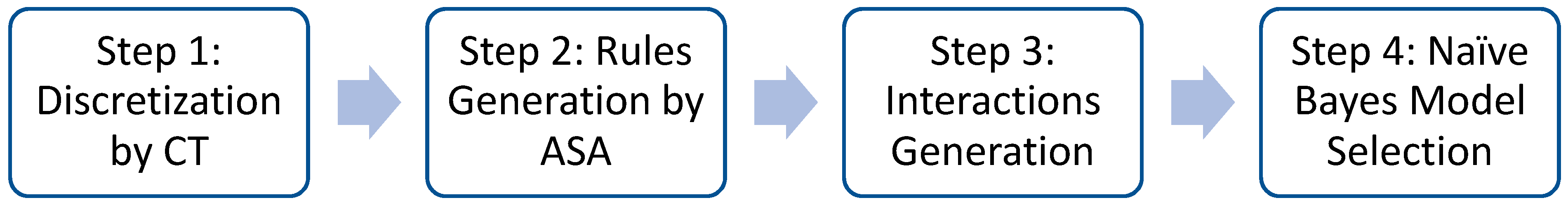
2.2. Proposed Method: Naïve Bayes Classifier Framework

The proposed framework for building a naïve Bayes classifier consists of four key steps (Figure 1).

The four steps in our framework are:

Step 1 (Discretization by CT): Utilize a classification tree to discretize each quantitative explanatory variable and convert each of them into a categorical variable.

Step 2 (Rules generation by ASA): Utilize CRM, a subset of ASA, to generate classifier rules from all the categorical variables, i.e., the new categorical variables generated in Step 1 and the original categorical variables.

Step 3 (Interactions generation): Generate the interactions for all the classifier rules in Step 2.

Step 4 (Naïve Bayes model selection): Select the optimal model for the naïve Bayes classifier—i.e., the one that provides the best value for our selection method—from all the original categorical variables, all the generated categorical variables in Step 1, and all the interactions generated in Step 3.

Step 1: Discretization by CT

As noted, we recommended a classification tree with weighting as the discretization method for our framework. In this step, we fitted the classification tree with each predictor as the sole predictor to find the splitting values. In turn, these values were used to partition the quantitative variable into levels as a basis for converting each quantitative variable into a categorical variable as needed.

Step 2: Rule Generation by ASA

In Step 2, we used CRM to create rules from the datasets. The candidate variables for generating the rules are (i) all the original categorical variables; and (ii) all the newly generated categorical variables from Step 1. This step is expected to result in rules in the form of “If X_i’s = x_i’s, then Y = y,” where x_i is the level of variable X_i and where y is the level of response Y. To perform the CRM, we used the classification based on associations (CBA) program developed by the Department of Information Systems and Computer Sciences at the National University of Singapore [19]. By simplifying the process, we used the classifier rules obtained from CBA, as shown in the following section. All classifier rules became the input for Step 3.

Step 3: Interactions Generation

In Step 3, we generated the interactions for the naïve Bayes classifier from the classifier rules generated in Step 2. We generated interactions between the items on the left-hand side with the same settings as those that appear in the rule. We assumed that the selected rule had three predictors in the form of “If X_i = x_i, X_j = x_j, and X_k = x_k, then Y = y,” where x_i is the level of variable X_i, x_j is the level of variable X_j, x_k is the level of variable X_k, and y is the level of response Y. We generated the interactions among X_i, X_j, and X_k by labeling each interaction as 1 if X_i = x_i, X_j = x_j, and X_k = x_k, and as 0 otherwise. This interaction is denoted X_i(x_i)X_j(x_j)X_k(x_k). For example, for the rule “If X₁ = 2, X₂ = 2, and X₃ = 1, then Y = 1,” we created an interaction among X₁, X₂, and X₃, denoted X₁(2)X₂(2)X₃(1). We have X₁(2)X₂(2)X₃(1) = 1 if X₁ = 2, X₂ = 2, and X₃ = 1, and 0 otherwise. The level of Y does not play any role in generating the variables. These interactions will be the candidate variables in Step 4.

Step 4: Naïve Bayes Model Selection

In Step 4, we selected the model for the naïve Bayes classifier by finding the set of predictors that give the best accuracy measure, which is the leave-one-out cross-validation method (LOOCV) or k-fold cross-validation with k = number of observations. The candidate variables are (i) the original categorical variables; (ii) the categorical variables generated in Step 1; and (iii) the interactions generated in Step 3.

3. Illustrated Examples

We demonstrated our methodology using three datasets: the thyroid dataset, the diabetes dataset, and the appendicitis dataset. Note that each of these three datasets initially comprised only quantitative predictors.

3.1. Thyroid Dataset

Retrieved from the University of California Irvine (UCI) machine learning site (https://archive.ics.uci.edu/ml/datasets/thyroid+disease, accessed on 11 February 2021), the dataset provided information on the thyroid function of 215 patients: 150 (69.77%) with normal function, 35 (16.28%) with hyperfunction, and 30 (13.95%) with hypofunction. There were five predictors in the dataset, all of which were quantitative variables (

Table 1. Predictors for the thyroid dataset.

Variable	N	Mean	Standard Deviation	Minimum	Median	Maximum
T3 RESIN	215	109.60	13.15	65.00	110.00	144.00
THYROXIN	215	9.81	4.70	0.50	9.20	25.30
THYRONINE	215	2.05	1.42	0.20	1.70	10.00
THYROID	215	2.88	6.12	0.10	1.30	56.40
TSH_VALUE	215	4.20	8.07	-0.70	2.00	56.30

). The objective of this analysis was to classify the patients as normal (Class 1), hyperfunction (Class 2), or hypofunction (Class 3).

We applied our approach to the thyroid dataset via the following steps.

Step 1 (Discretization by CT): We discretized the five quantitative variables into categories using a classification tree. We fitted the model to predict the response, using one variable at a time, and thus obtaining the splitting values for each quantitative variable.

The classification model in which T3 resin was used as a predictor to classify the response yielded two splitting values: 99.5 and 117.5. Therefore, we generated the categorical variable by discretizing T3 resin (X1), which has three levels (

Table 2. Discretized variables generated using the classification tree method: thyroid dataset.

Original Variable	Discretized Variable	Detail
T3 resin	X1	X1 = 1 if T3 resin < 99.5
		X1 = 2 if 99.5 ≤ T3 resin < 117.5
		X1 = 3 if T3 resin ≥ 117.5
Thyroxine	X2	X2 = 1 if thyroxine < 5.65
		X2 = 2 if 5.65 ≤ thyroxine < 12.65
		X2 = 3 if thyroxine ≥ 12.65
Thyronine	X3	X3 = 1 if thyronine < 1.15
		X3 = 2 if 1.15 ≤ thyronine < 2.65
		X3 = 3 if thyronine ≥ 2.65
Thyroid	X4	X4 = 1 if thyroid < 0.75
		X4 = 2 if 0.75 ≤ thyroid < 1.05
		X4 = 3 if 1.05 ≤ thyroid < 1.15
		X4 = 4 if 1.15 ≤ thyroid < 1.45
		X4 = 5 if 1.45 ≤ thyroid < 1.65
		X4 = 6 if 1.65 ≤ thyroid < 1.75
		X4 = 7 if 1.75 ≤ thyroid < 1.85
		X4 = 8 if 1.85 ≤ thyroid < 4
		X4 = 9 if thyroid ≥ 4
TSH-value	X5	X5 = 1 if TSH-value < 0.65
		X5 = 2 if 0.65 ≤ TSH-value < 4.45
		X5 = 3 if TSH-value ≥ 4.45

).

The classification model in which thyroxine was used as a predictor to classify the response yielded two splitting values: 5.65 and 12.65. Therefore, we generated the categorical variable by discretizing thyroxin (X2), which has three levels (Table 2).

The classification model in which thyronine was used as a predictor to classify the response yielded two splitting values: 1.15 and 2.65. Therefore, we generated the categorical variable by discretizing thyronine (X3), which has three levels (Table 2).

The classification model in which thyroid was used as a predictor to classify the response yielded eight splitting values: 0.75, 1.05, 1.15, 1.45, 1.65, 1.75, 1.85, and 4.0. Therefore, we generated the categorical variable by discretizing thyroid (X4), which has nine levels (Table 2).

The classification model in which the TSH-value was used as a predictor to classify the response yielded two splitting values: 0.65 and 4.45. Therefore, we generated the categorical variable by discretizing the TSH-value (X5), which has three levels (Table 2).

Step 2 (Rules generation by ASA): We used CBA to obtain the classifier rules. In this step, the variables inputted into the process were the original categorical predictors (X1–X5). In total, 21 classifier rules were generated in this step (

Table 3. Classifier rules generated by CBA: thyroid dataset.

No.	Rules	Generated Interactions
1	If X5 = 2 and X2 = 2, then Y = 1	X5(2)X2(2) = 1 if X5 = 2 and X2 = 2
		X5(2)X2(2) = 0, otherwise
2	If X5 = 2 and X3 = 2, then Y = 1	X5(2)X3(2) = 1 if X5 = 2 and X3 = 2
		X5(2)X3(2) = 0, otherwise
3	If X4 = 2 and X2 = 2, then Y = 1	X4(2)X2(2) = 1 if X4 = 2 and X2 = 2
		X4(2)X2(2) = 0, otherwise
4	If X5 = 2 and X4 = 2, then Y = 1	X5(2)X4(2) = 1 if X5 = 2 and X4 = 2
		X5(2)X4(2) = 0, otherwise
5	If X4 = 4 and X2 = 2, then Y = 1	X4(4)X2(2) = 1 if X4 = 4 and X2 = 2
		X4(4)X2(2) = 0, otherwise
6	If X3 = 3 and X2 = 3, then Y = 2	X3(3)X2(3) = 1 if X3 = 3 and X2 = 3
		X3(3)X2(3) = 0, otherwise
7	If X4 = 9, then Y = 3	X4(9) = 1 if X4 = 9
		X4(9) = 0, otherwise
8	If X5 = 3 and X2 = 1, then Y = 3	X5(3)X2(1) = 1 if X5 = 3 and X2 = 1
		X5(3)X2(1) = 0, otherwise
9	If X2 = 3 and X1 = 1, then Y = 2	X2(3)X1(1) = 1 if X2 = 3 and X1 = 1
		X2(3)X1(1) = 0, otherwise
10	If X4 = 5 and X3 = 2, then Y = 1	X4(5)X3(2) = 1 if X4 = 5 and X3 = 2
		X4(5)X3(2) = 0, otherwise
11	If X3 = 3 and X1 = 1, then Y = 2	X3(3)X1(1) = 1 if X3 = 3 and X1 = 1
		X3(3)X1(1) = 0, otherwise
12	If X4 = 8 and X3 = 2, then Y = 1	X4(8)X3(2) = 1 if X4 = 8 and X3 = 2
		X4(8)X3(2) = 0, otherwise
13	If X3 = 1 and X2 = 1, then Y = 3	X3(1)X2(1) = 1 if X3 = 1 and X2 = 1
		X3(1)X2(1) = 0, otherwise
14	If X4 = 8 and X1 = 2, then Y = 1	X4(8)X1(2) = 1 if X4 = 8 and X1 = 2
		X4(8)X1(2) = 0, otherwise
15	If X4 = 1 and X2 = 3, then Y = 2	X4(1)X2(3) = 1 if X4 = 1 and X2 = 3
		X4(1)X2(3) = 0, otherwise
16	If X4 = 1 and X1 = 1, then Y = 2	X4(1)X1(1) = 1 if X4 = 1 and X1 = 1
		X4(1)X1(1) = 0, otherwise
17	If X4 = 3 and X3 = 3, then Y = 2	X4(3)X3(3) = 1 if X4 = 3 and X3 = 3
		X4(3)X3(3) = 0, otherwise
18	If X3 = 2, X2 = 2, and X1 = 2, then Y = 1	X3(2)X2(2)X1(2) = 1 if X3 = 2, X2 = 2, and X1 = 2
		X3(2)X2(2)X1(2) = 0, otherwise
19	If X5 = 2 and X1 = 2, then Y = 1	X5(2)X1(2) = 1 if X5 = 2 and X1 = 2
		X5(2)X1(2) = 0, otherwise
20	If X2 = 2 and X1 = 2, then Y = 1	X2(2)X1(2) = 1 if X2 = 2 and X1 = 2
		X2(2)X1(2) = 0, otherwise
21	If X5 = 1 and X2 = 3, then Y = 2	X5(1)X2(3) = 1 if X5 = 1 and X2 = 3
		X5(1)X2(3) = 0, otherwise

).

Step 3 (Interactions generation): We converted the 21 classifier rules into interactions. In total, 21 interactions were generated from the 21 classifier rules (Table 3).

Note that the first rule has support (s) = 0.4884 and confidence (c) = 1, which means that P(X5 = 2, X2 = 2, and Y = 1) = 0.4884 and P(X5 = 2, X2 = 2, and Y = 1)/P(X5 = 2 and X2 = 2) = 1.

Step 4 (Naïve Bayes model selection): We combined the 21 interactions with the other discretized variables (X1–X5) to generate 26 candidate predictors for naïve Bayes. We searched for the model that gave the best LOOCV accuracy. We selected the model with all the discretized variables X1–X5 and the first 19 interactions shown in Table 3. The LOOCV value generated by this model was 99.53%.

3.2. Diabetes Dataset

Originally from the National Institute of Diabetes and Digestive and Kidney Diseases, the diabetes dataset was retrieved from Kaggle (https://www.kaggle.com/uciml/pima-indians-diabetes-database, accessed on 17 February 2021). In this dataset, eight quantitative variables were used to classify patients as either healthy or diabetic [21]. With 768 observations, there were 500 healthy patients (Class 0) and 268 patients with diabetes (Class 1). In this data, 65.1% of the observations belonged to Class 0 and 34.9% belonged to Class 1. There were eight predictors in the dataset, all of which were quantitative variables (

Table 4. Predictors for the diabetes dataset.

Variable	N	Mean	Standard Deviation	Minimum	Median	Maximum
Pregnancies	768	3.85	3.37	0.00	3.00	17.00
Glucose	768	120.89	31.97	0.00	117.00	199.00
Blood pressure	768	69.11	19.36	0.00	72.00	122.00
Skin thickness	768	20.54	15.95	0.00	23.00	99.00
Insulin	768	79.80	115.24	0.00	30.50	846.00
BMI	768	31.99	7.88	0.00	32.00	67.10
Diabetes pedigree function	768	0.47	0.33	0.08	0.37	2.42
Age	768	33.24	11.76	21.00	29.00	81.00

). The objective of this analysis was to classify the patients as healthy (Class 0) or diabetic (Class 1).

We applied our approach to the diabetes dataset via the follow steps.

Step 1 (Discretization by CT): We discretized the eight quantitative variables into categories using a classification tree. The discretized variables are shown in

Table 5. Discretized variables generated by the classification tree: diabetes dataset.

Original Variable	Discretized Variable	Detail
Pregnancies	X1	X1 = 1 if pregnancies < 6.5
		X1 = 2 if pregnancies ≥ 6.5
Glucose	X2	X2 = 1 if glucose < 99.5
		X2 = 2 if 99.5 ≤ glucose < 111.5
		X2 = 3 if 111.5 ≤ glucose < 114.5
		X2 = 4 if 114.5 ≤ glucose < 115.5
		X2 = 5 if 115.5 ≤ glucose < 123.5
		X2 = 6 if 123.5 ≤ glucose < 125.5
		X2 = 7 if 125.5 ≤ glucose < 126.5
		X2 = 8 if 126.5 ≤ glucose < 127.5
		X2 = 9 if 127.5 ≤ glucose < 152.5
		X2 = 10 if 152.5 ≤ glucose < 154.5
		X2 = 11 if glucose ≥ 154.5
Blood pressure	X3	X3 = 1 if blood pressure < 42
		X3 = 2 if 42 ≤ blood pressure < 69
		X3 = 3 if 69 ≤ blood pressure < 71
		X3 = 4 if 71 ≤ blood pressure < 73
		X3 = 5 if 73 ≤ blood pressure < 74.5
		X3 = 6 if 74.5 ≤ blood pressure < 75.5
		X3 = 7 if 75.5 ≤ blood pressure < 79
		X3 = 8 if 79 ≤ blood pressure < 81
		X3 = 9 if blood pressure ≥ 81
Skin thickness	X4	X4 = 1 if skin thickness < 7.5
		X4 = 2 if 7.5 ≤ skin thickness < 31.5
		X4 = 3 if skin thickness ≥ 31.5
Insulin	X5	X5 = 1 if insulin < 14.5
		X5 = 2 if 14.5 ≤ insulin < 87.5
		X5 = 3 if 87.5 ≤ insulin < 91.5
		X5 = 4 if 91.5 ≤ insulin < 95.5
		X5 = 5 if 95.5 ≤ insulin < 99.5
		X5 = 6 if 99.5 ≤ insulin < 121
		X5 = 7 if insulin ≥ 121
BMI	X6	X6 = 1 if BMI < 27.85
		X6 = 2 if 27.85 ≤ BMI < 29.85
		X6 = 3 if 29.85 ≤ BMI < 40.05
		X6 = 4 if 40.05 ≤ BMI < 40.85
		X6 = 5 if BMI ≥ 40.85
Diabetes pedigree function	X7	X7 = 1 if diabetes pedigree function < 0.21
		X7 = 2 if 0.21 ≤ diabetes pedigree function < 0.28
		X7 = 3 if 0.28 ≤ diabetes pedigree function < 0.32
		X7 = 4 if 0.32 ≤ diabetes pedigree function < 0.38
		X7 = 5 if 0.38 ≤ diabetes pedigree function < 0.52
		X7 = 6 if 0.52 ≤ diabetes pedigree function < 0.53
		X7 = 7 if diabetes pedigree function ≥ 0.53
Age	X8	X8 = 1 if age < 28.5
		X8 = 2 if 28.5 ≤ age < 62.5
		X8 = 3 if age ≥ 62.5

.

Step 2 (Rules generation by ASA): We used CBA to obtain the classifier rules. In this step, the variables inputted into the process were the original categorical predictors (X1–X8). In total, 77 classifier rules were generated in this step.

Step 3 (Interactions generation): We converted the 77 classifier rules into interactions. In total, 77 interactions were generated from the 77 classifier rules.

Given the high number of rules and interactions generated, we presented only the first 10 rules and the interactions they generated in

Table 6. First 10 classifier rules generated by CBA: diabetes dataset.

No.	Rules	Generated Interactions
1	If X6 = 1, X2 = 1, and X1 = 1, then Y = 0	X6(1)X2(1)X1(1) = 1 if X6 = 1, X2 = 1, and X1 = 1
		X6(1)X2(1)X1(1) = 0, otherwise
2	If X4 = 2, X3 = 2, and X2 = 1, then Y = 0	X4(2)X3(2)X2(1) = 1 if X4 = 2, X3 = 2, and X2 = 1
		X4(2)X3(2)X2(1) = 0, otherwise
3	If X6 = 1, X4 = 2, and X2 = 1, then Y = 0	X6(1)X4(2)X2(1) = 1 if X6 = 1, X4 = 2, and X2 = 1
		X6(1)X4(2)X2(1) = 0, otherwise
4	If X5 = 2, X3 = 2, and X2 = 1, then Y = 0	X5(2)X3(2)X2(1) = 1 if X5 = 2, X3 = 2, and X2 = 1
		X5(2)X3(2)X2(1) = 0, otherwise
5	If X8 = 1, X7 = 1, and X6 = 1, then Y = 0	X8(1)X7(1)X6(1) = 1 if X8 = 1, X7 = 1, and X6 = 1
		X8(1)X7(1)X6(1) = 0, otherwise
6	If X8 = 1, X5 = 1, and X2 = 2, then Y = 0	X8(1)X5(1)X2(2) = 1 if X8 = 1, X5 = 1, and X2 = 2
		X8(1)X5(1)X2(2) = 0, otherwise
7	If X8 = 2, X7 = 7, X2 = 11, and X1 = 2, then Y = 1	X8(2)X7(7)X2(11)X1(2) = 1 if X8 = 2, X7 = 7, X2 = 11, and X1 = 2
		X8(2)X7(7)X2(11)X1(2) = 0, otherwise
8	If X5 = 7, X2 = 11, and X1 = 2, then Y = 1	X5(7)X2(11)X1(2) = 1 if X5 = 7, X2 = 11, and X1 = 2
		X5(7)X2(11)X1(2) = 0, otherwise
9	If X6 = 3, X5 = 1, X2 = 11, and X1 = 1, then Y = 1	X6(3)X5(1)X2(11)X1(1) = 1 if X6 = 3, X5 = 1, X2 = 11, and X1 = 1
		X6(3)X5(1)X2(11)X1(1) = 0, otherwise
10	If X6 = 1 and X2 = 1, then Y = 0	X6(1)X2(1) = 1 if X6 = 1 and X2 = 1
		X6(1)X2(1) = 0, otherwise

.

Step 4 (Naïve Bayes model selection): We combined the 77 interactions with the other discretized variables (X1–X8) to generate 85 candidate predictors for naïve Bayes. We searched for the model that gave the best LOOCV value. We selected the model with X1, X2, X5, X6, X7, and X8 and the interaction generated from Rule 2, which is X4(2)X3(2)X2(1). The LOOCV value from this model was 81.25%.

3.3. Appendicitis Dataset

Retrieved from the KEEL website (https://sci2s.ugr.es/keel/dataset.php?cod=183, accessed on 21 April 2021), the appendicitis dataset comprised seven medical measures to classify patients according to whether or not they had appendicitis. In 106 observations, there were 85 healthy patients (Class 0) and 21 patients who had appendicitis (Class 1). In the data, 80.19% of the observations belonged to Class 0 and 19.81% belonged to Class 1. There were seven predictors in the dataset, all of which were quantitative variables (

Table 7. Predictors for the appendicitis dataset.

Variable	N	Mean	Standard Deviation	Minimum	Median	Maximum
WBC1	106	0.40	0.19	0.00	0.41	1.00
MNEP	106	0.68	0.21	0.00	0.75	1.00
MNEA	106	0.42	0.21	0.00	0.44	1.00
MBAP	106	0.21	0.20	0.00	0.15	1.00
MBAA	106	0.17	0.18	0.00	0.11	1.00
HNEP	106	0.68	0.22	0.00	0.74	1.00
HNEA	106	0.38	0.20	0.00	0.40	1.00

). The objective of this analysis was to classify the patients as healthy (Class 0) or as having appendicitis (Class 1).

We applied our approach to the appendicitis dataset via the following steps:

Step 1 (Discretization by CT): We discretized the seven quantitative variables into categories using a classification tree. The discretized variables are shown in

Table 8. Discretized variables generated by the classification tree: appendicitis dataset.

Original Variable	Discretized Variable	Detail
WBC1	X1	X1 = 1 if WBC1 < 0.2155
		X1 = 2 if 0.2155 ≤ WBC1 < 0.362
		X1 = 3 if 0.362 ≤ WBC1 < 0.3845
		X1 = 4 if 0.3845 ≤ WBC1 < 0.942
		X1 = 5 if WBC1 ≥ 0.942
MNEP	X2	X2 = 1 if MNEP < 0.42
		X2 = 2 if 0.42 ≤ MNEP < 0.509
		X2 = 3 if 0.509 ≤ MNEP < 0.5625
		X2 = 4 if 0.5625 ≤ MNEP < 0.598
		X2 = 5 if 0.598 ≤ MNEP < 0.616
		X2 = 6 if 0.616 ≤ MNEP < 0.652
		X2 = 7 if 0.652 ≤ MNEP < 0.741
		X2 = 8 if 0.741 ≤ MNEP < 0.8125
		X2 = 9 if MNEP ≥ 0.8125
MNEA	X3	X3 = 1 if MNEA < 0.2315
		X3 = 2 if MNEA ≥ 0.2315
MBAP	X4	X4 = 1 if MBAP < 0.007
		X4 = 2 if 0.007 ≤ MBAP < 0.021
		X4 = 3 if 0.021 ≤ MBAP < 0.035
		X4 = 4 if 0.035 ≤ MBAP < 0.049
		X4 = 5 if 0.049 ≤ MBAP < 0.0625
		X4 = 6 if 0.0625 ≤ MBAP < 0.104
		X4 = 7 if 0.104 ≤ MBAP < 0.132
		X4 = 8 if 0.132 ≤ MBAP < 0.16
		X4 = 9 if 0.16 ≤ MBAP < 0.3125
		X4 = 10 if 0.3125 ≤ MBAP < 0.34
		X4 = 11 if 0.34 ≤ MBAP < 0.5695
		X4 = 12 if 0.5695 ≤ MBAP < 0.59
		X4 = 13 if MBAP ≥ 0.59
MBAA	X5	X5 = 1 if MBAA < 0.0535
		X5 = 2 if MBAA ≥ 0.0535
HNEP	X6	X6 = 1 if HNEP < 0.509
		X6 = 2 if 0.509 ≤ HNEP < 0.6685
		X6 = 3 if 0.6685 ≤ HNEP < 0.757
		X6 = 4 if HNEP ≥ 0.757
HNEA	X7	X7 = 1 if HNEA < 0.1475
		X7 = 2 if 0.1475 ≤ HNEA < 0.215
		X7 = 3 if 0.215 ≤ HNEA < 0.2435
		X7 = 4 if 0.2435 ≤ HNEA < 0.343
		X7 = 5 if 0.343 ≤ HNEA < 0.365
		X7 = 6 if 0.365 ≤ HNEA < 0.432
		X7 = 7 if 0.432 ≤ HNEA < 0.4365
		X7 = 8 if 0.4365 ≤ HNEA < 0.9185
		X7 = 9 if HNEA ≥ 0.9185

.

Step 2 (Rules generation by ASA): We used CBA to obtain the classifier rules. In this step, the variables inputted into the process were the original categorical predictors (X1–X7). In total, 10 classifier rules were generated in this step.

Step 3 (Interactions generation): We converted the 10 classifier rules into interactions. In total, 10 interactions were generated from the 10 classifier rules, as shown in

Table 9. Classifier rules generated by CBA: appendicitis dataset.

No.	Rules	Generated Interactions
1	If X6 = 4 and X5 = 2, then Y = 0	X6(4)X5(2) = 1 if X6 = 4 and X5 = 2
		X6(4)X5(2) = 0, otherwise
2	If X6 = 2 and X3 = 2, then Y = 0	X6(2)X3(2) = 1 if X6 = 2 and X3 = 2
		X6(2)X3(2) = 0, otherwise
3	If X4 = 5 and X1 = 1, then Y = 1	X4(5)X1(1) = 1 if X4 = 5 and X1 = 1
		X4(5)X1(1) = 0, otherwise
4	If X7 = 3 and X5 = 2, then Y = 1	X7(3)X5(2) = 1 if X7 = 3 and X5 = 2
		X7(3)X5(2) = 0, otherwise
5	If X7 = 3 and X6 = 3, then Y = 1	X7(3)X6(3) = 1 if X7 = 3 and X6 = 3
		X7(3)X6(3) = 0, otherwise
6	If X7 = 7 and X2 = 7, then Y = 1	X7(7)X2(7) = 1 if X7 = 7 and X2 = 7
		X7(7)X2(7) = 0, otherwise
7	If X4 = 3 and X2 = 8, then Y = 1	X4(3)X2(8) = 1 if X4 = 3 and X2 = 8
		X4(3)X2(8) = 0, otherwise
8	If X5 = 1 and X1 = 1, then Y = 1	X5(1)X1(1) = 1 if X5 = 1 and X1 = 1
		X5(1)X1(1) = 0, otherwise
9	If X6 = 1 and X1 = 1, then Y = 1	X6(1)X1(1) = 1 if X6 = 1 and X1 = 1
		X6(1)X1(1) = 0, otherwise
10	If X7 = 1 and X1 = 1, then Y = 1	X7(1)X1(1) = 1 if X7 = 1 and X1 = 1
		X7(1)X1(1) = 0, otherwise

.

Step 4 (Naïve Bayes model selection): We combined 10 interactions with the other discretized variables (X1–X7) to generate 17 candidate predictors for naïve Bayes. We searched for the model that gave the best LOOCV value. We selected the model with X7 and all 10 interactions shown in Table 9. The LOOCV value from this model was 95.28%.

4. Performance Comparison via Medical Datasets

In this section, we describe our application of the other well-known classification methods to the thyroid, diabetes, and appendicitis datasets in order to compare their performance with our methodology.

A comparison of the performance of the five methods is shown in

Table 10. LOOCV accuracy (%) for the five methods tested.

Medical Dataset	Random Forest		SVM		kNN	Classification Tree	CT+ASA+NB
	Ntree	Accuracy	Kernel	Accuracy	Accuracy	Accuracy	Accuracy
Thyroid	100	96.74	sigmoid	93.95	96.28	93.95	99.53
	200	97.21	linear	96.27
	500	96.28	poly	91.16
	1000	96.28	radial	95.81
Diabetes	100	76.30	sigmoid	69.66	74.87	78.12	81.25
	200	77.08	linear	77.08
	500	76.95	poly	74.74
	1000	76.69	radial	75.78
Appendicitis	100	87.74	sigmoid	78.30	87.74	84.91	95.28
	200	87.74	linear	87.74
	500	86.79	poly	86.79
	1000	86.79	radial	86.79

. The five methods tested are as follows: (1) random forest (RF); (2) support vector machine (SVM); (3) k-nearest neighbors (kNN); (4) classification tree (CT); and (5) naïve Bayes (NB) with classification tree (CT) and ASA, which is our approach (NB + CT + ASA). The comparison is shown through the LOOCV accuracy.

For random forest, we set the number of trees (ntree) according to four levels: 100, 200, 500, and 1000. Then, for each number of trees, we searched for the best LOOCV value among all the numbers of variables considered at each split, as indicated in Table 10.

For SVM, the LOOCV value, as shown in Table 10, was found for each of the four kernel types: the sigmoid kernel, the linear kernel, the polynomial kernel, and the radial basis kernel.

For kNN, the indicated LOOCV accuracy value shown in Table 10 is the highest for all the odd numbers of neighbors (k) from 1 to 19.

For the classification tree, the LOOCV accuracy value shown in Table 10 was obtained from the number of splits that gave the best LOOCV value among all possible numbers.

As shown in Table 10, our approach provided the highest LOOCV value of all the methods for all three medical datasets, with the most impressive performance shown for the appendicitis dataset.

5. Discussion and Conclusions

Our naïve Bayes model selection framework provides a classifier that significantly outperformed the other well-known data mining techniques tested, i.e., classification tree, random forest, kNN, and SVM. Our approach has an advantage over the other methods in that it can be used to generate interactions through ASA—an unconventional way of generating interactions by finding the combinations of the levels of the variables that are important for predicting the class for the categorical responses. In particular, ASA is effective at finding the combinations of the levels of variables that appear frequently and strongly for each of the classes of the response through selected rules. The model’s effectiveness in this regard is very helpful for working with unbalanced datasets such as the thyroid and appendicitis datasets. Moreover, our experiments with the different discretization methods showed the classification tree to be the most effective for our approach.

We demonstrated that the integration of three techniques—classification tree, ASA, and the naïve Bayes classifier—constituted a superior and practical classifier. Based on our application examples, it is evident that these newly generated variables and interactions made a significant contribution to improving the naïve Bayes classifier.

References

1. Al-Aidaroos, K.M.; Bakar, A.A.; Othman, Z. Medical data classification with Naïve Bayes approach. Inf. Technol. J. 2012, 11, 1166–1174. [Google Scholar] [CrossRef] [Green Version]
2. Golpour, P.; Ghayour-Mobarhan, M.; Saki, A.; Esmaily, H.; Taghipour, A.; Tajfard, M.; Ghazizadeh, H.; Moohebati, M.; Ferns, G.A. Comparison of support vector machine, Naïve Bayes and logistic regression for assessing the necessity for coronary angiography. Int. J. Environ. Res. Public Health 2020, 17, 6449. [Google Scholar] [CrossRef] [PubMed]
3. Langarizadeh, M.; Moghbeli, F. Applying Naïve Bayesian networks to disease prediction: A systematic review. Acta Inform. Med. 2016, 24, 364–369. [Google Scholar] [CrossRef] [PubMed]
4. Miasnikof, P.; Giannakeas, V.; Gomes, M.; Aleksandrowicz, L.; Shestopaloff, A.Y.; Alam, D.; Tollman, S.; Samarikhalaj, A.; Jha, P. Naïve Bayes classifiers for verbal autopsies: Comparison to physician-based classification for 21,000 child and adult deaths. BMC Med. 2015, 13, 286. [Google Scholar] [CrossRef] [PubMed] [Green Version]
5. Al-Aidaroos, K.M.; Bakar, A.A.; Othman, Z. Naïve Bayes Variants in Classification Learning. In Proceedings of the 2010 International Conference on Information Retrieval & Knowledge Management (CAMP), Shah Alam, Malaysia, 17–18 March 2010; Institute of Electrical and Electronics Engineers (IEEE): Shah Alam, Malaysia, 2010; pp. 276–281. [Google Scholar]
6. Melingi, S.; Vijayalakshmi, V. An effective approach for sub-acute ischemic stroke lesion segmentation by adopting meta-heuristics feature selection technique along with hybrid Naïve Bayes and sample-weighted random forest classification. Sens. Imaging 2019, 20, 7. [Google Scholar]
7. Jiang, L.; Wang, D.; Cai, Z.; Yan, X. Survey of improving Naive Bayes for classification. In Advanced Data Mining and Applications. ADMA 2007. Lecture Notes in Computer Science; Alhajj, R., Gao, H., Li, J., Li, X., Zaïane, O.R., Eds.; Springer: Berlin/Heidelberg, Germany, 2007; Volume 4632, pp. 134–145. [Google Scholar]
8. Farid, D.; Zhang, L.; Rahman, C.; Hossain, M.; Strachan, R. Hybrid decision tree and Naïve Bayes classifiers for multi-class classification tasks. Expert Syst. Appl. Int. J. 2014, 41, 1937–1946. [Google Scholar] [CrossRef]
9. Abraham, R.; Simha, J.; Iyengar, S. Effective discretization and hybrid feature selection using Naïve Bayesian classifier for medical datamining. Int. J. Comput. Intell. Res. 2008, 4, 974–1259. [Google Scholar] [CrossRef]
10. Huang, Z.; Zhou, Z.; He, T. Resolving rule conflicts based on Naïve Bayesian model for associative classification. J. Digit. Inform. Manag. 2014, 12, 36–43. [Google Scholar]
11. Hadi, W.; Al-Radaideh, Q.; Alhawari, S. Integrating associative rule-based classification with Naïve Bayes for text classification. Appl. Soft Comput. 2018, 69, 344–356. [Google Scholar] [CrossRef]
12. Bressan, M.; Vitrià, J. Improving Naïve Bayes using class-conditional ICA. In Advances in Artificial Intelligence, IBERAMIA 2002. Lecture Notes in Computer Science; Garijo, F.J., Riquelme, J.C., Toro, M., Eds.; Springer: Berlin/Heidelberg, Germany, 2002; Volume 3, pp. 1–10. [Google Scholar]
13. Domingos, P.; Pazzani, M. On the optimality of the simple Bayesian classifier under zero-one loss. Mach. Learn. 1997, 29, 103–130. [Google Scholar] [CrossRef]
14. Changpetch, P.; Reid, M. Data mining techniques: Which one is your favorite? J. Educ. Bus. 2021, 96, 143–148. [Google Scholar] [CrossRef]
15. Berry, M.J.A.; Linoff, G. Data Mining Techniques: For Marketing, Sales, and Customer Support, 3rd ed.; John Wiley & Sons: Indianapolis, IN, USA, 1997. [Google Scholar]
16. Changpetch, P.; Lin, D.K.J. Model selection for logistic regression via association rules analysis. J. Stat. Comput. Simul. 2013, 83, 1415–1428. [Google Scholar] [CrossRef]
17. Changpetch, P.; Lin, D.K.J. Selection for multinomial logit models via association rules analysis. WIREs Comput. Stat. 2013, 5, 68–77. [Google Scholar] [CrossRef]
18. Agrawal, R.; Srikant, S. Fast Algorithms for Mining Association Rules. In VLDB’94, Proceedings of the 20th International Conference on Very Large Data Bases, Santiago de Chile, Chile, 12–15 September 1994; Bocca, J.B., Jarke, M., Zaniolo, C., Eds.; Morgan Kaufmann: San Francisco, CA, USA, 1994; pp. 487–499. [Google Scholar]
19. Liu, B.; Hsu, W.; Ma, Y. Integrating Classification and Association Rule Mining. In KDD-98, Proceedings of the Fourth International Conference on Knowledge Discovery and Data Mining, New York, NY, USA, 27–31 August 1998; Agrawal, R., Stolorz, P.E., Piatetsky-Shapiro, G., Eds.; AAAI Press: Menlo Park, CA, USA, 1998; pp. 80–86. [Google Scholar]
20. Quinlan, J.R. C4.5: Programs for Machine Learning; Morgan Kaufmann: San Francisco, CA, USA, 1992. [Google Scholar]
21. Smith, J.W.; Everhart, J.E.; Dickson, W.C.; Knowler, W.C.; Johannes, R.S. Using the ADAP Learning Algorithm to Forecast the Onset of Diabetes Mellitus. In Proceedings of the Symposium on Computer Applications in Medical Care, Minneapolis, MN, USA, 8–10 June 1988; Greenes, R.A., Ed.; IEEE Computer Society Press: Los Alamitos, CA, USA, 1988; pp. 261–265. [Google Scholar]
Figure 1. Naïve Bayes classifier framework.
Computation 09 00099 g001