
Forecasting Multivariate Chaotic Processes with Precedent Analysis

1
Saint-Petersburg State Institute of Technology, Technical University, St. Petersburg Institute for Informatics and Automation of the Russian Academy of Sciences, 190013 St. Petersburg, Russia
2
Department of Computing Systems and Computer Science, Admiral Makarov State University of Maritime and Inland Shipping, 198035 St. Petersburg, Russia
3
Center for Econometrics and Business Analytics, Saint-Petersburg State University, 199034 St. Petersburg, Russia
*
Author to whom correspondence should be addressed.
Computation 2021, 9(10), 110; https://0-doi-org.brum.beds.ac.uk/10.3390/computation9100110
Submission received: 4 September 2021
/
Revised: 11 October 2021
/
Accepted: 13 October 2021
/
Published: 19 October 2021
(This article belongs to the Section Computational Engineering)
Abstract
:Predicting the state of a dynamic system influenced by a chaotic immersion environment is an extremely difficult task, in which the direct use of statistical extrapolation computational schemes is infeasible. This paper considers a version of precedent forecasting in which we use the aftereffects of retrospective observation segments that are similar to the current situation as a forecast. Furthermore, we employ the presence of relatively stable correlations between the parameters of the immersion environment as a regularizing factor. We pay special attention to the choice of similarity measures or distances used to find analog windows in arrays of retrospective multidimensional observations.
1. Introduction
In many practical problems, a complex oscillatory non-periodic process that contains local trends and jumps describes the change in the parameters of the observed system. The corresponding observation series usually implements chaotic processes [1,2,3,4,5]; examples include turbulent flows in unstable gas-dynamic and hydrodynamic environments [6,7,8], changes in asset prices at electronic capital markets [9,10,11], as well as many others.
In some cases, the dynamics of deterministic chaos can be described by a system of open non-linear differential equations, the solution of which is a non-periodic oscillatory process containing a large number of bifurcation points. The presence of such points leads to extremely insignificant fluctuations of external influences able to cause a significant and poorly predictable change in the integral curve. In practice, the ambiguity of the mathematical descriptions of such processes is intensified by the presence of a random component, which is due to many factors that are not taken into account in the mathematical model of the system component of the observed process.
The modern approach to dynamic system management is based on proactivity, characterized by a preemptive action directed onto the control object, which presupposes the presence of a predicted scenario of the situation. In this regard, the central place in solving a complex control problem is occupied by predicting the state of the observed object, which includes the prediction of changes in its immersion environment.
The above complexities of the mathematical description of chaotic dynamics of systems immersed in unstable interaction environments significantly complicate the qualitative solutions of the forecasting problem. In particular, the studies in [12,13,14] demonstrate the unsuitability of traditional methods of statistical extrapolation for predicting the state of low-inertia processes. The authors of [11,12,13,14,15] propose algorithms for forecasting chaotic processes based on precedent forecasting. They are based on a typical hypothesis of cognitive computing and machine learning: similar (referring to a similarity metric) situations are followed by similar aftereffects.
This article continues research into multidimensional immersion environments. The presence of relatively stable correlations between the parameters of the observed process is used as a regularizing factor. The similarity of the observation windows of a multidimensional process is estimated based on vector proximity measures (similarity metrics or pseudometrics).
The study of the issues of precedent forecast construction for multidimensional chaotic processes and a comparative analysis of the options for its implementation constitute the content of this work.
2. Materials and Methods
Let Y<m:1>(k), k = 1, …, N be an m-dimensional series of observations captured by a system that monitors the parameters of a real process occurring in an unstable immersion environment. As the observation model, we use a conventional additive relation of the form
where X<m:1>(k) is the so-called systemic component used to make management decisions and v<m:1>(k) is a random process that simulates observation noise. The systemic component X(k) is supposed to be the output of some non-linear system with determined coefficients and initial values. However, severe dependence of the output on initial conditions has caused the observer to be unable to predict the behavior of the system without any prior knowledge. Several approaches in this area including model-based and data-driven classifications, are regarded in [16,17,18,19,20]. Particularly, in [20], the authors regard methods of multidimensional sparse regression to identify relevant terms in the system component X(k) (SINDy).
Y(k) = X(k) + v(k), k = 1, …, N
Here, we examine a highly narrow problem statement and a number of other model classes are proposed, for example, in [1,2,3,4,5]. In terms of the geometry of observation space, we consider it to be approximately flat.
The main feature of this problem is that the system component Xi(k), i = 1, …, m is an implementation of multidimensional dynamic chaos. Moreover, each of its parameters is an oscillatory non-periodic process that contains pronounced local trends. Usually, the system component X(k), k = 1, …, N is isolated from the mix Y(k), k = 1,…, N by sequential filtration. However, it is very difficult to strictly separate deterministic and random components under these conditions. This requires the introduction of additional subjective constraints.
Random component v <m:1>(k) represents an m-dimensional noise process that is not taken into account in the decision-making process and is subject to filtering. Generally, it is close to the Wiener process, however, it significantly deviates from the stationarity condition due to the presence of heteroscedasticity and random variations of the autocorrelation function. The Gaussian condition is also satisfied very approximately due to a large number of abnormal observations and the failure to conform to the regularizing conditions of the central limit theorems [21,22].
Another feature of the problem is that the elements of vector Yi(k), i = 1, …, m significantly correlate. In this case, the proposed relative stability (that has to be investigated individually) of the values of the covariance matrix P(Y) = cov(Yi,Yj), i,j = 1, …, m makes it possible to use this property as a regularizing factor in precedent forecasting. This assumption must be checked by analyzing the dynamics of pairwise correlations on sliding windows. Stability, here, is connected with the correctness of the proposed approximate flatness and must be checked for the data of interest.
Let there be an array of training historical data , in which is an m-dimensional vector of observations and NS. is the size of the training sample. In the case of the continuous monitoring of the observed object, this array can be continuously replenished directly adjacent to the current moment in time.
On time interval , the values of the process parameters are sequentially forecasted for a time interval of counts. It is required to obtain the forecasted estimates with an accuracy level that is acceptable from the point of view of the higher-level management task. This accuracy can be estimated, for example, with a quadratic indicator.
The forecast effectiveness evaluation usually consists of obtaining the prediction accuracy of the forecasted parameter only. The remaining m − 1 parameters of the state vector are used only for generating similarity metrics and searching for analog windows.
The traditional approach to forecasting non-stationary processes involves constructing a sliding window of the current state of L counts in size, directly adjacent to the current moment of time
in which a predictive model that maps is constructed with statistical analysis methods.
This approach, which has many adaptive and robust versions, provides satisfactory results for small values of the prediction horizon for observation series (1) corresponding to a typical model with an unknown deterministic systemic component and stationary noise. However, in the considered problem, the systemic component of observations is an implementation of deterministic chaos. In such conditions, this approach, as shown in [12,13,14], does not produce acceptable accuracy levels. Even when using a simplified criterion of forecast effectiveness, which is an estimate of the frequency of correctly predicted linear trend directions, the frequency of correct decisions in the extrapolation forecast was at about 50%. In other words, the reliability of the forecast tends to its potential minimum.
In this regard, following [11,12,13,14,15], this paper considers the possibility of constructing a precedent forecast, but, in contrast to this work, the algorithm for predicting the selected parameter takes into account the multidimensionality of the observed chaotic process, the parameters of which are correlated with each other.
The forecasting algorithm proposed in the work can be described with the following sequential computational scheme:
1. Using a sliding scan window
at each k-th step of forecasting, the algorithm scans the array of retrospective data with an increment and calculates the values of similarity metrics
The size of the observation window in conventional statistical studies is estimated using the minimization of the mean square of the error, which includes both the standard deviation and the amount of displacement caused by dynamic errors. However, for chaotic environments, this approach is unacceptable due to the non-stationarity of the observation series. The size of the state window should be considered as an option to be refined in the process of adapting the model.
2. After the scan is complete, the algorithm searches for analog windows with numbers that correspond to the smallest values of the similarity measure. The scan window (4) with the minimum value of the similarity metric is considered a precedent.
3. As already noted, the aftereffect following the precedent window is used as a forecast
that is, following the scan window with the minimum value of the selected metric
To increase the stability of the result, the average value of the aftereffects following the found analog windows can be used as a forecast.
A natural choice of vector similarity metrics is the distance relations used in multivariate statistical analysis and machine learning problems. In more common cases, it may be reasonable to use special metrics developed for chaos, such as the largest Lyapunov exponents and Lyapunov spectrum, fractal dimension, Kolmogorov–Sinai entropy, etc. Therefore, it is not surprising that in statistical classification, the most widespread measures are vector analogs of the quadratic distance, such as the Euclidean distance
or, for correlated data, the Mahalanobis distance
in which are the estimates of the average values for the scan window (4) and the average over the entire training sample, and is a sample covariance matrix.
If the covariance matrix is an identity matrix, the Mahalanobis distance coincides with the Euclidean distance. If the covariance matrix is diagonal (but not necessarily unitary), the resulting distance measure is called the normalized Euclidean distance.
Quadratic metrics are closely related to the -Hotelling distribution and are widely used in statistical classification problems, in multidimensional statistical testing, in Fisher’s linear discriminant analysis, and in supervised machine learning.
It should be noted that in multivariate analysis, any hypothesis can have a large set of alternatives, thus there are no criteria that are uniformly optimal with respect to cardinality. Various numerical characteristics of matrices or , where are the sample covariance matrices of the samples under consideration on the observation windows (3) and (4), are used as analogues of Fischer’s F-statistic.
Let the eigenvalues of the matrix be and the eigenvalues of matrix be . In variance analysis, the following statistics are the most common [23]:
- (1)
- Hotelling (or Lawley–Hotelling) trace:
- (2)
- Hotelling’s statistic:
- (3)
- Pillai’s trace:
- (4)
- Roy’s characteristic roots:
- (5)
- Wilkes’ statistic:
The distributions of these statistics for various null hypotheses are quite complicated. In practice, these distributions are usually approximated by the F-distribution with a particular choice of the number of degrees of freedom. All the statistics given can be interpreted as distances in the corresponding pseudometrics. Historically, they are called information distances. Particular attention should be paid to the Kullback–Leibler distance that determines the degree of similarity of two probability distributions, namely and , in the common space of observations Y.
Let and , where is an arbitrary measure on Y. Then, the Kullback–Leibler divergence is defined as . In some cases, is interpreted as a relative entropy of with respect to . For two multivariate normal distributions, namely and , the Kullback–Leibler distance can be written as a combination of the previously described proximity measures in the form or in terms of statistics (11, 14),
Strictly speaking, the given metric is not a distance as it does not satisfy the triangle inequality and is not symmetrical.
At the same time, in the class of information metrics, the Kullback–Leibler distance has a number of important optimal properties.
3. Results
3.1. Multidimensional Data Polygon for Studying the Effectiveness of Forecasting Algorithms: Preliminary Studies
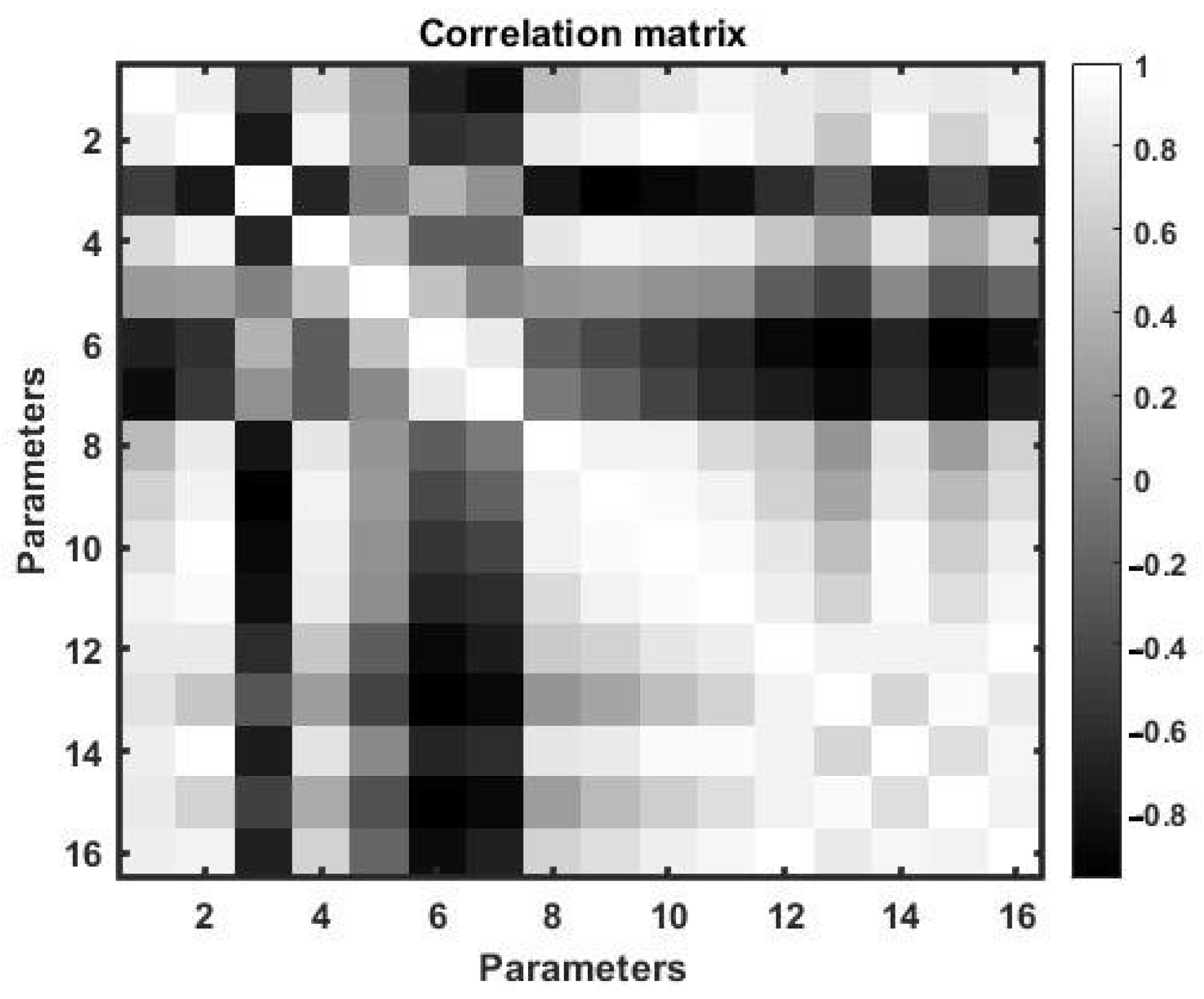
We used normalized observations of 16 parameters of the distributed undulating hydrodynamic flow as a polygon for multivariate correlated data. One of these parameters, for example, parameter 1, is subject to forecasting, and nP = 3 parameters, which are most correlated with the forecasted one, are selected from the remaining parameters using correlation analysis.
To select these parameters, we estimated the matrix of pairwise correlations over a large interval of training observations with a duration of 432,000 min counts.
Figure 1 shows a two-dimensional tonal matrix that displays the values of paired correlation coefficients. The figure shows that the parameters with the numbers are the most correlated with the first parameter.
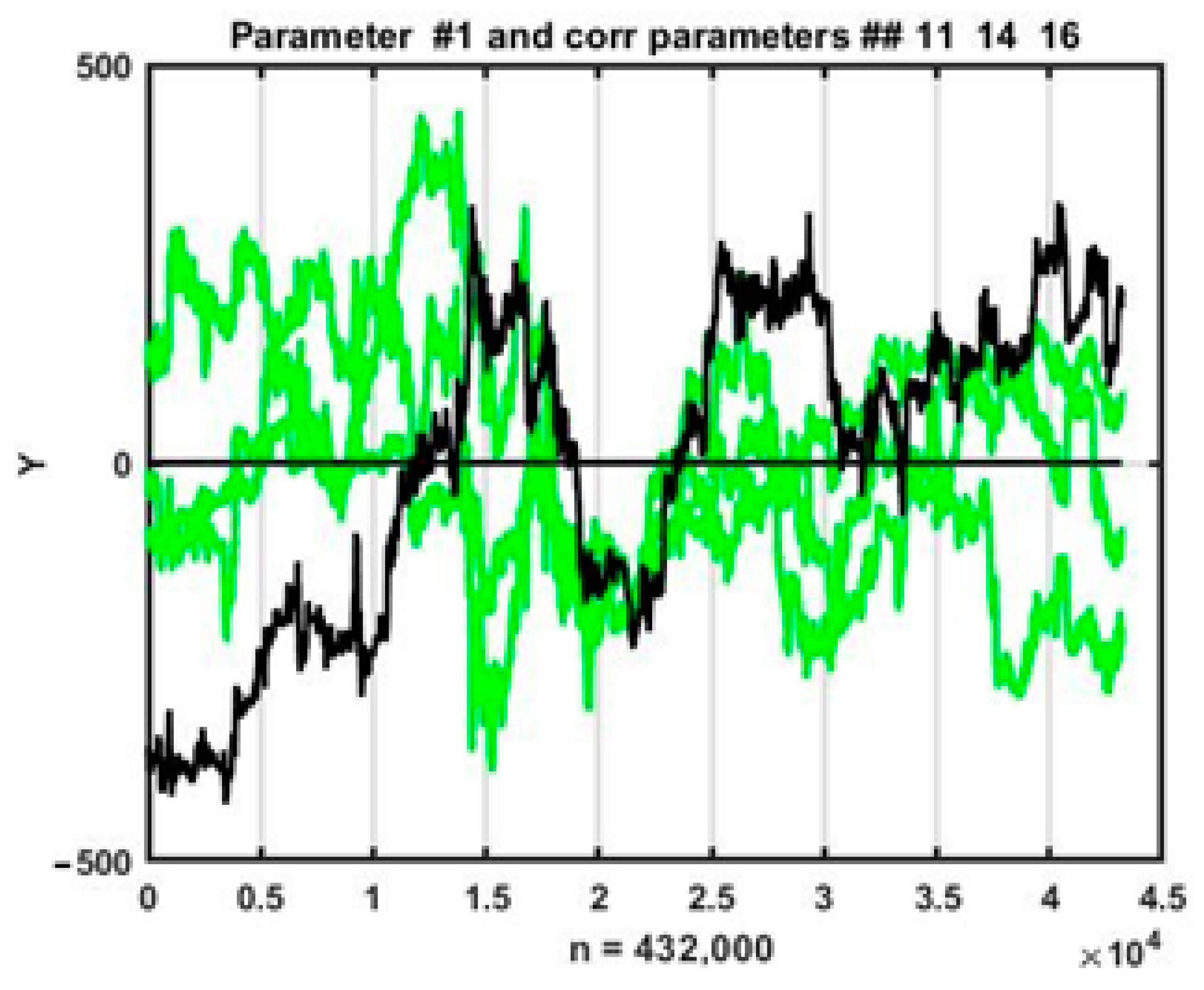
Figure 2 shows time plots of changes in all four parameters on a time interval of 432,000 counts that were used for training in the process of searching for analogs of the current situation. It can be seen from the plots above that the parameter behavior for a multidimensional chaotic process is highly fluctuating, which inevitably affects changes in the estimates of pairwise coefficients at local observation segments. Nevertheless, in general, parameter trend directions coincide in most cases.
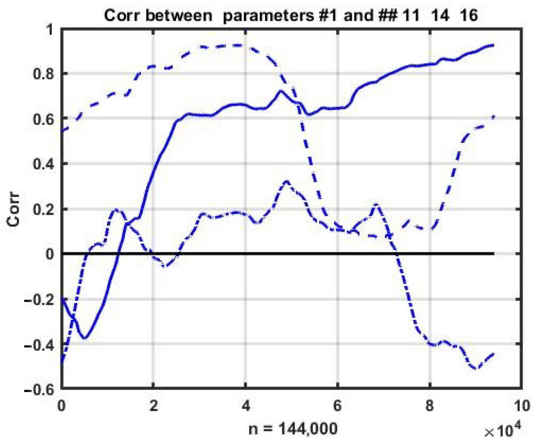
This observation requires numerical confirmation of the relative stability of correlations. In order to achieve this, we estimated the change dynamics of pairwise correlations within a sliding observation window. The corresponding plots of the correlations between the first parameter and the other three (11, 14, and 16) are shown in Figure 3.
It can be seen that the process is purely non-stationary and the correlations between the parameters change continuously and within a wide range. Nevertheless, the rate of change in correlations is significantly lower than the variability of the observed processes, which allows us to assume the possibility of using multidimensional relationships as a regularizing factor for constructing short-term forecasts.
3.2. Property Analysis of Similarity Measures in Chaotic Processes
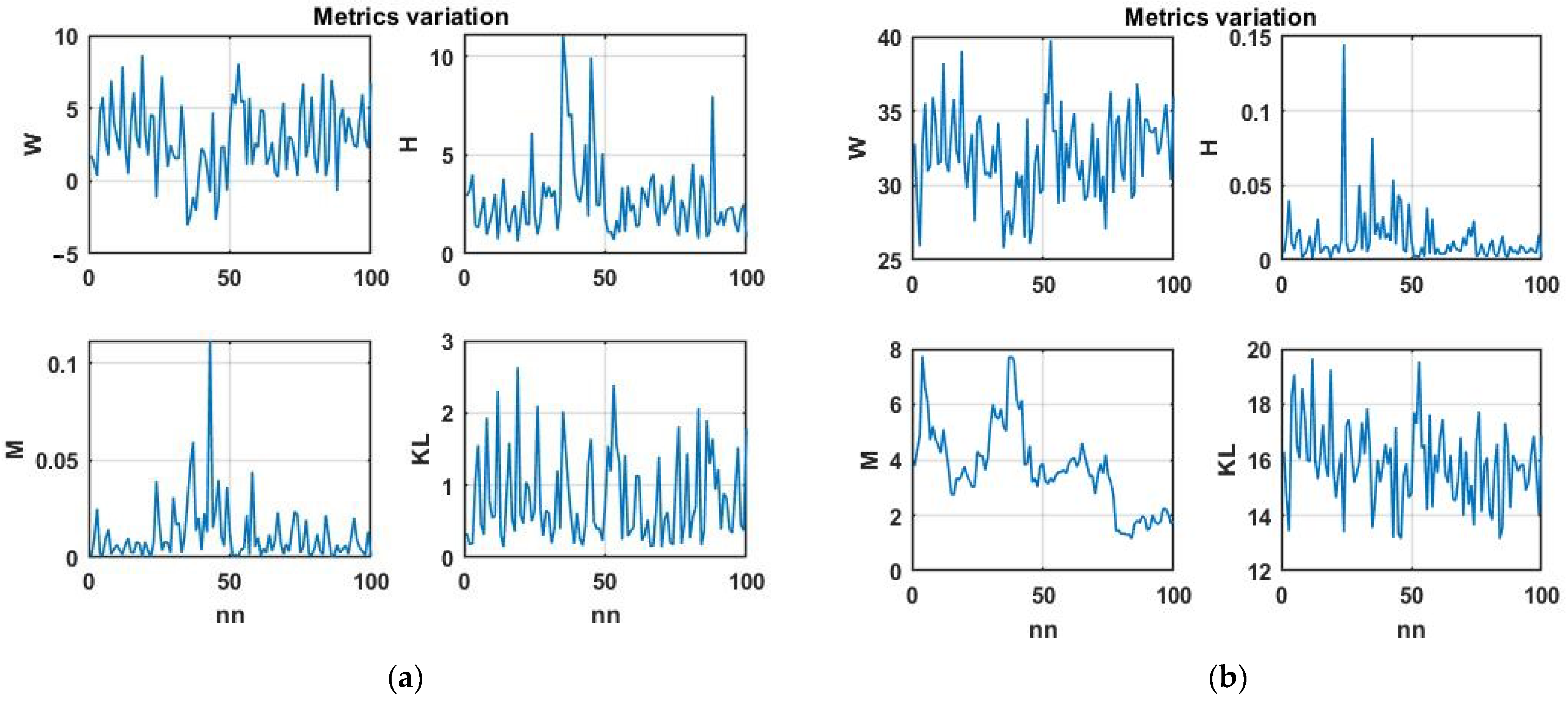
Initially, we considered the change dynamics of the Wilkes’ statistic (14), Hotelling distance (11), Kullback–Leibler distance (15), and modified Mahalanobis distance (9). We used the four-dimensional chaotic process shown in Figure 2 as the initial data. Figure 4a shows the corresponding plots of changes in similarity metrics for the first difference of a multidimensional chaotic process and Figure 4b does so for the process itself.
The plots show that the Wilkes and Kullback–Leibler statistics have a certain normalizing effect, bringing them closer to white noise. This effect is of interest from the point of view of theoretical statistics; however, it complicates their use for searching for analog situations.
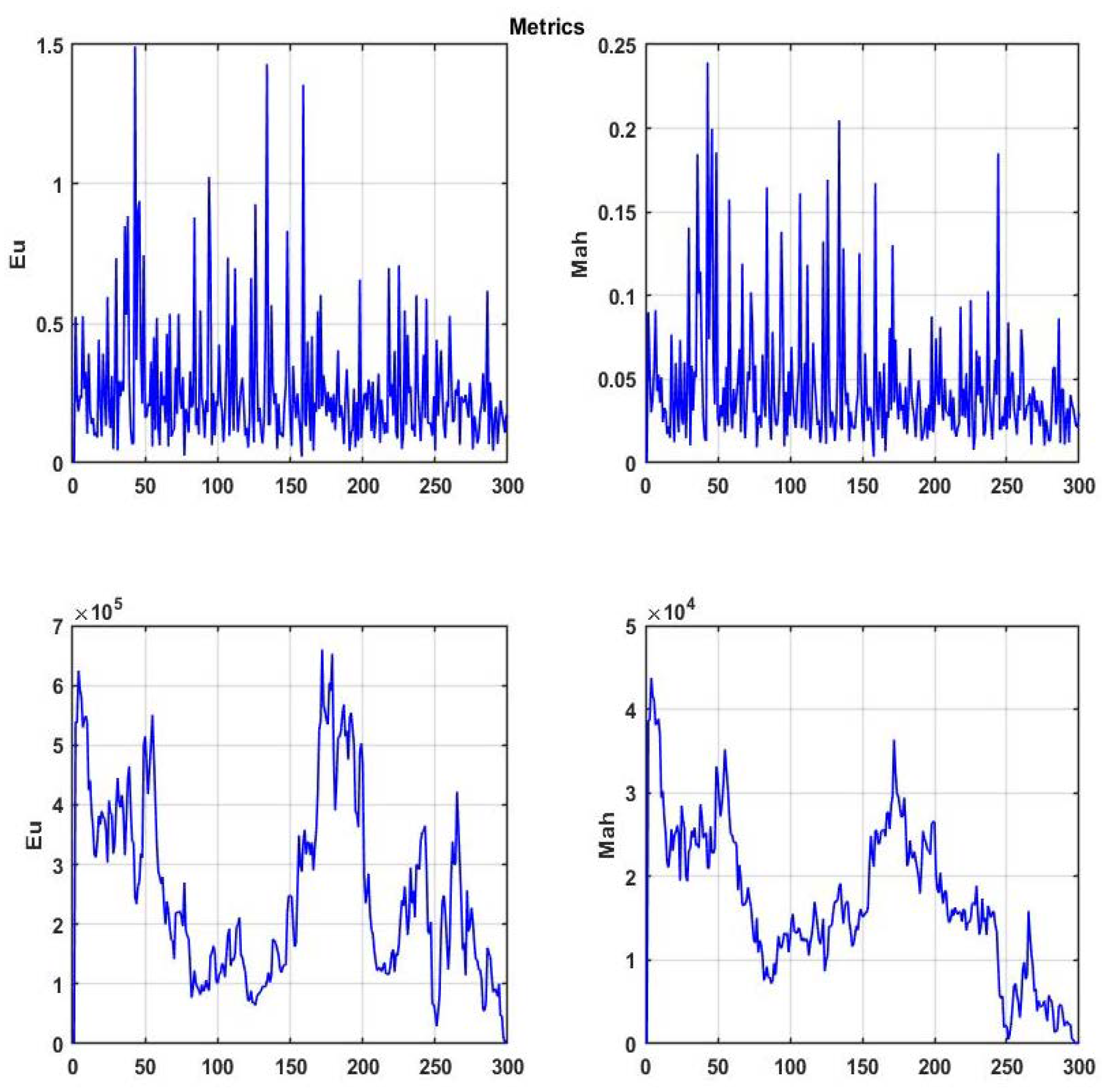
Taking into account correlations in identifying analog situations makes it possible to increase the decision effectiveness by using important additional information about the interdependence of the parameters at the current time. However, the stochastic nature of variations in the estimates of correlations over time (see Figure 3), which significantly increases with the decreasing scan window size, can introduce additional uncertainty into the problem. In this regard, we preliminarily considered the problem of assessing the significance of correlations by comparing the dynamics of changes in Euclidean (8) and Mahalanobis metrics (9), which differ only in terms of the presence of a correlation matrix.
Figure 5 shows plotted changes in these measures for a sliding observation window with a size of 200 counts at 300 scanning steps of a multidimensional chaotic process. The top plots show the result for the first differences and the bottom ones show the result for the chaotic process itself.
It is easy to see that the transition to the first differences brings the observed process closer to a stationary one and, for both metrics, decreases their capability of identifying areas with the greatest degree of similarity.
When using a chaotic process properly, both similarity measures tend to zero at the final stage of observation. This is because the average of the scan window approaches the average value of the current situation window. Hence, it follows that the specified segment should be excluded from the analog situation search area. In addition, it can be seen from the same plots that taking into account the correlations between the parameters changes the dynamics of the similarity measure. However, their significance for solving the problems of precedent forecasting can be assessed only via a comparative statistical study based on terminal estimates of the accuracy of the resulting forecast.
From the plotted dynamics of metrics changing over time as presented in Figure 4 and Figure 5, it can be seen that all of them have a high level of randomness, which will not only complicate the search for analog situations but can also lead to erroneous conclusions. Therefore, it is advisable to move from the original values of these metrics to their smoothed values.
To smooth the data, we used the simplest exponential filter
with transmission ratio that provides a compromise between the degree of smoothing and the magnitude of the resulting sequential estimate bias.
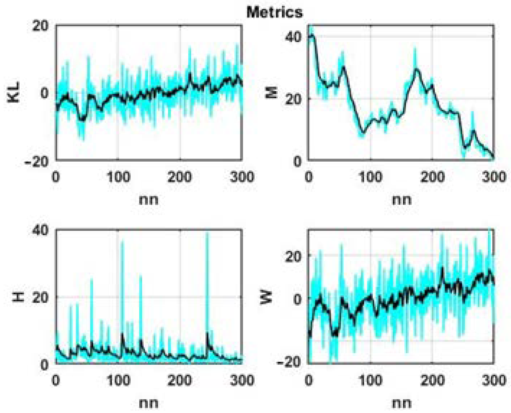
The smoothing results for the four considered statistics are shown in Figure 6.
Note that initially the range of variation of the presented measures differed by several orders of magnitude. As a result, the dynamics of the Kullback–Leibler statistic, calculated as the sum (15), were completely determined by the values of the Mahalanobis statistic (9). Due to this, we used normalizing coefficients to preserve the significance of all additive components in (15).
The plots presented in Figure 5 and Figure 6 allow us to draw the following intermediate conclusions. With significant fluctuations in the level of the observed process, the Euclidean and Mahalanobis distances will be completely determined by the difference between the mean values of the state window and scanning windows, and the values at the end of the scanning interval; when these windows approach each other, these distances will naturally decrease. This means that in the given formulation of the problem, these distances are not feasible for searching for analogs using the degree of statistical similarity between the current state and the data in scan windows.
Therefore, within the framework of our studies, we decided to focus on the problem of precedent analysis based on metrics that exclusively measure the similarity of the correlation properties of processes in observation windows.
3.3. Analog Search in Multidimensional Chaotic Processes
The detection of analogs for the current state of a stochastic system, i.e., similar vector situations in a time-ordered array of retrospective data, as well as the corresponding aftereffects used as prognostic estimates, was carried out in accordance with (2–7).
We will denote an analog situation corresponding to the smallest value of the distance in the selected similarity metric (6) as a precedent. Initially, we considered the problem of finding analogs with the Hotelling (11) and Wilkes (14) measures based on the similarity of correlations in the observation windows.
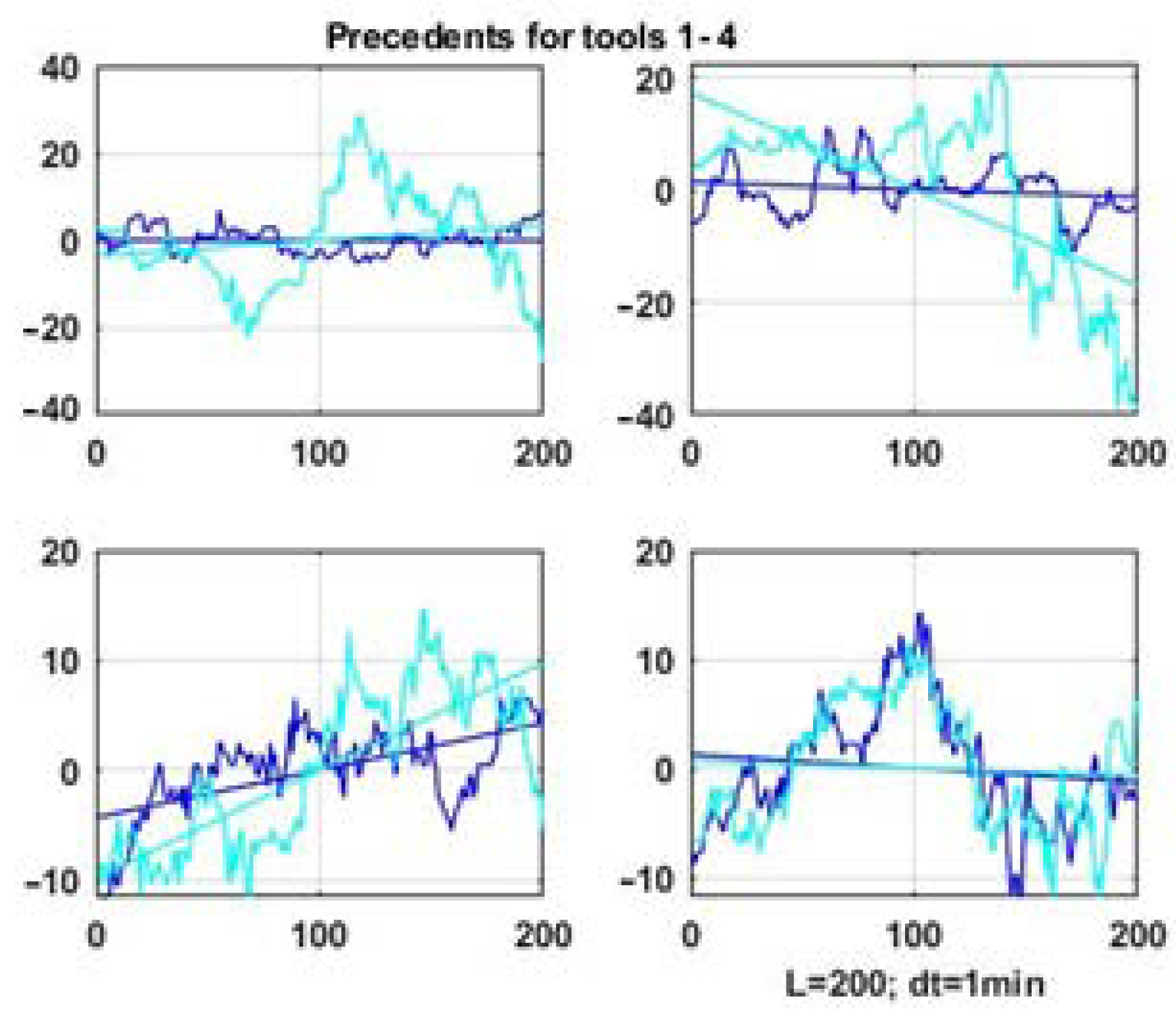
Let us consider, as an example, a precedent search result (i.e., an analog window with the highest level of vector similarity) for each of the four parameters of the chaotic process. The search was carried out in an array of retrospective data of counts. The correlation matrix was sequentially evaluated on a sliding scan window of counts and shift of the scanning window was counts.
Figure 7 shows precedent windows, i.e., the vector window with the highest degree of similarity by the Hotelling statistic, for four parameters of a multidimensional chaotic process. The data of the scan window is emphasized with a darker color compared to the data segment of their status window.
It is obvious that it is not possible to achieve geometric similarity as it was done for the one-dimensional problem in [6] considering the similarity criterion is based on the degree of proximity of correlation matrix functionals. At best, we can expect the similarity of linear trends, which are also presented in Figure 7 and Figure 8 as straight lines representing linear approximations of the processes observed in the windows.
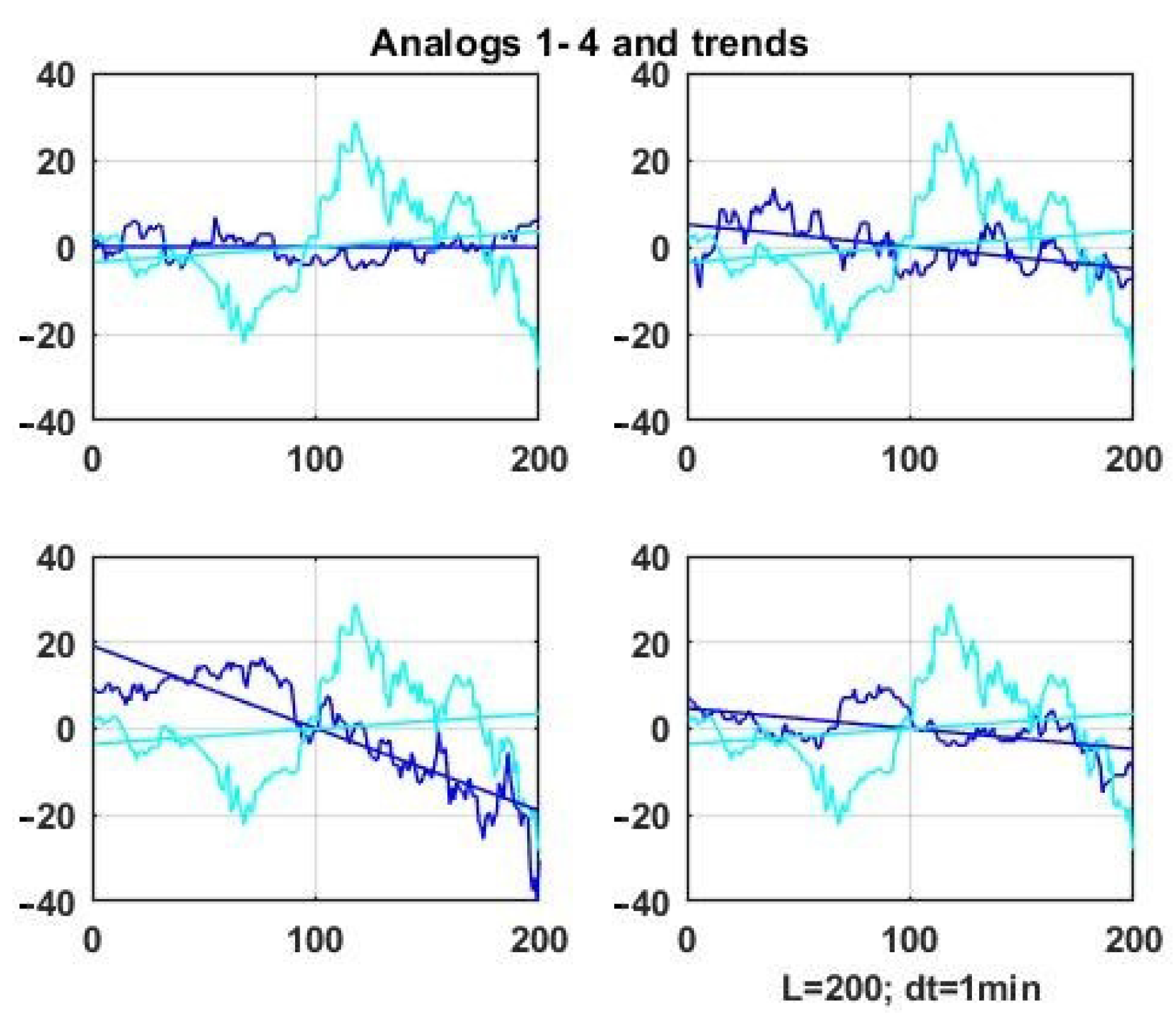
Figure 8 shows similar results for four analog windows for the first parameter of the vector chaotic process (darker lines) compared to the observation series in the current state window.
Analogous similarity plots can be obtained using expressions (10, 12, and 13) based on the correlation matrix as the similarity metric.
It can be seen that the similarity of the correlation structures does not guarantee the geometric similarity of the processes in the compared observation windows, as was the case in the examples in [11,12,13,14,15]. Moreover, even the similarity of linear trends is not guaranteed for multidimensional chaos. In the theory of machine observation, such computational schemes are placed in the category of weak classifiers [24,25,26,27].
Nevertheless, this does not allow us to conclude that it is inadmissible to use the considered method in precedent forecasting. The relevance of studying this issue is due to the lack of alternatives among the traditional methods of statistical extrapolation for predicting the state of multidimensional chaotic processes.
3.4. Precedent Forecasting in Multidimensional Chaotic Processes: Numerical Studies
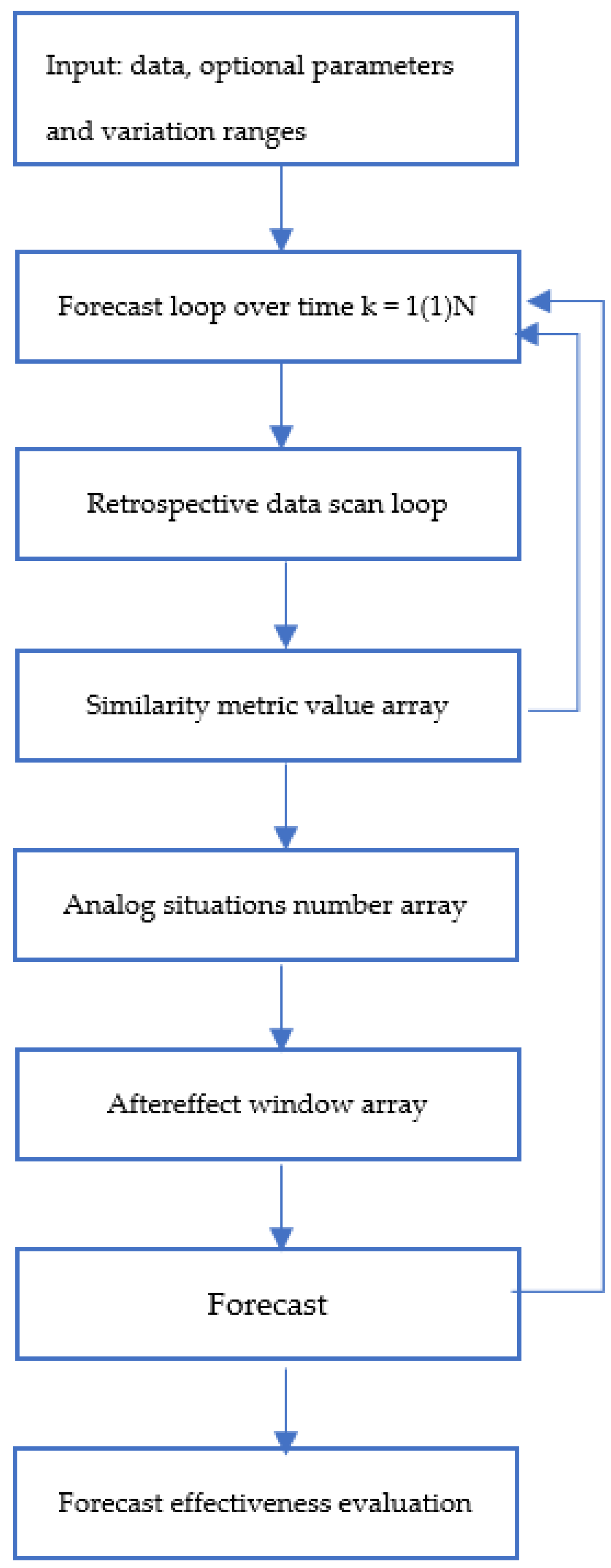
The block diagram of a precedent forecast implementation for a multidimensional chaotic process is shown in Figure 9.
The search for analog windows ends with identifying their scan numbers corresponding to the smallest values of the similarity measure in the training historical dataset. As already noted, the forecast uses the aftereffect (5) following the precedent window or the average value of the aftereffects following the found analog windows (7).
To study the effectiveness of precedent forecasting, following the results of sections 7 and 8, we used similarity metrics based on Hotelling (11) and Wilkes (14) statistics.
Two examples of implementing a multidimensional precedent forecast using these metrics are shown in Figure 10.
From the above plots, we can see a relatively low degree of geometric similarity between the posteriorly observed forecast and its forecasts. The reason for this is that the choice of precedents and consequently their aftereffects used as a forecast for both metrics do not take into account the degree of geometric similarity. This leads to a mismatch between the similarity criterion and the traditional assessment of the forecast quality (2). Nevertheless, these results may be useful as an element of the swarm intelligence approach [17,18,19,20,21]. This issue will be examined in more detail in the Discussion section.
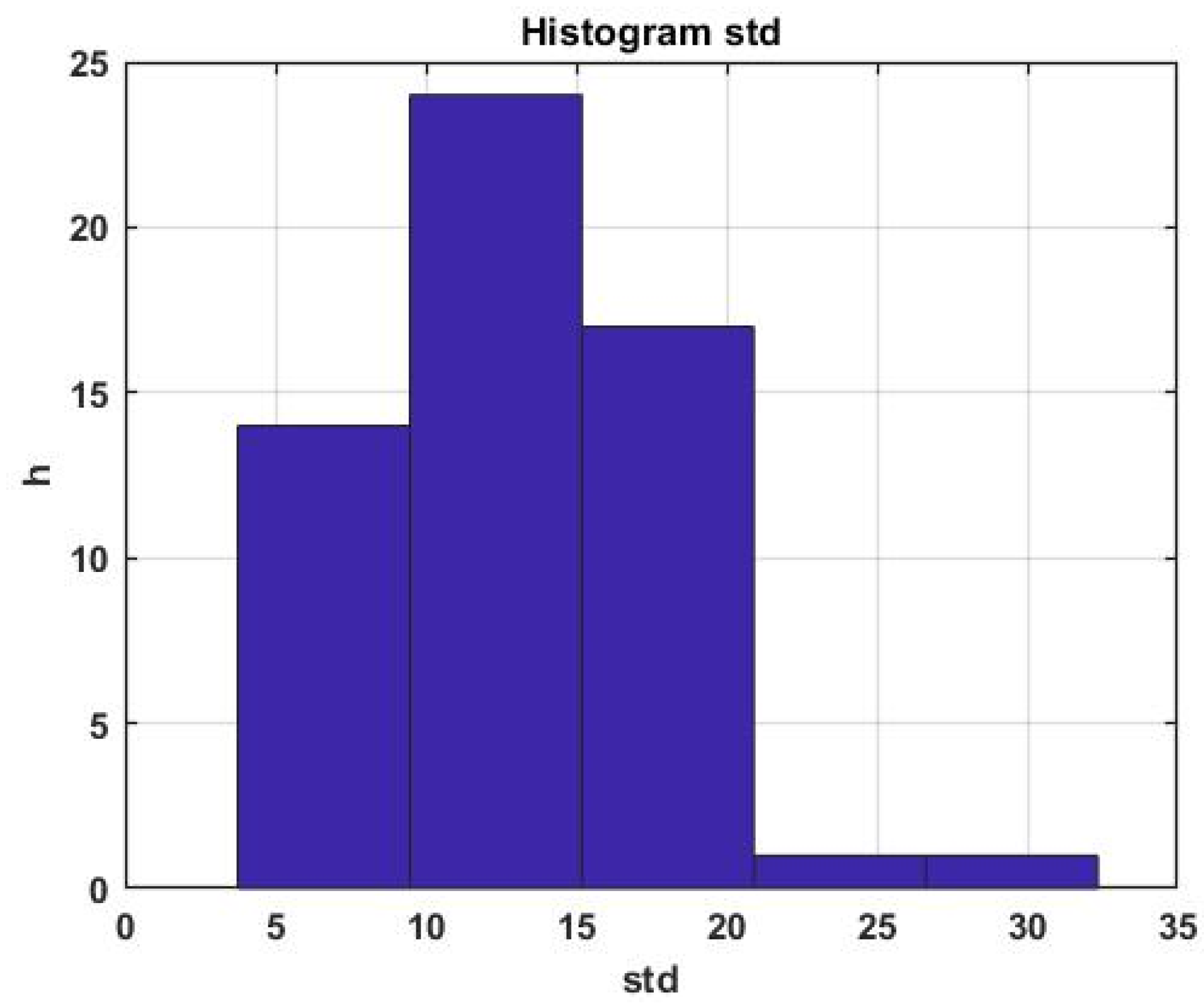
To quantify the prediction accuracy, we initially used the ratio (2) calculated at each prediction step with selected scan window size L and the window shift. The SD estimate is random, usually slowly converging to a normal distribution.
An example of a histogram of the SD distribution for the first parameter of a multidimensional process is shown in Figure 11.
It can be seen that the scatter of the estimate relative to the average is quite large, which is inevitable, taking into account the chaotic nature of the forecasted process. It is obvious that in order to assess the quality of forecasting over the entire interval of sequential forecast estimates, it is necessary to switch to the average value of the standard error of the forecast, specifically
where , is the number of prediction steps.
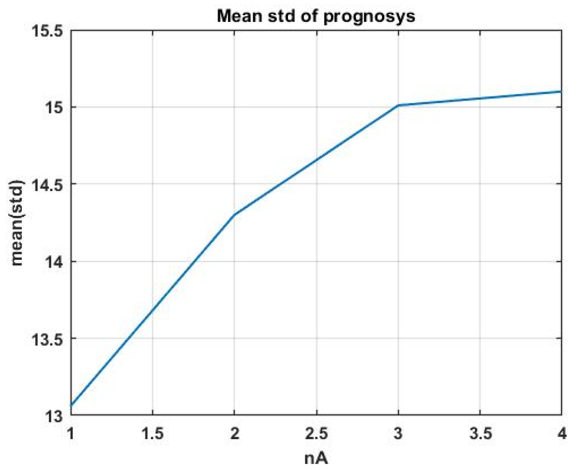
Using indicator (17), we considered the question of the fundamental suitability of precedent analysis for constructing a forecast in chaotic environments. For this purpose, let us consider the dependence of the average of SD on the number of the analog window. An increase in the number means a lower degree of similarity of the analog window and therefore a lower similarity of the aftereffect to the forecasted interval. Figure 12 shows the solution of this problem for four analog windows when using the Hotelling statistic as a similarity measure (11).
The resulting plot confirms the fundamental suitability of the considered forecasting technology. However, the final decision should be made based on the achieved forecast accuracy, complying with the requirements of the task in the interests of which this forecast is made.
It is obvious that the accuracy of the generated forecast depends on the parameters of the used algorithm. In this case, such parameters are the size of the scan window that matches the size of the current situation window, scan shift, forecast interval , and, if the search for analogs is performed on smoothed data, filtering coefficient . In addition, various similarity metrics can be used in the process of finding the best decision, which will require additional structuring of the forecasting program.
It should be noted that the forecasting interval is not always an option; in many applied problems, it is determined by the requirements of the metasystem that implements the obtained forecast.
The above results provide a significant increase in accuracy (about 25% and higher when switching to the search for analog windows for pre-smoothed data (for example, using an exponential filter (16)) by constructing a forecast to average the aftereffects for analog windows (7).
In addition, it is possible to increase the accuracy of the forecast, provided that there are regularizing factors in the initial series of observations themselves, by applying sequential parametric and structural adaptation. In particular, the work [28] presents an adaptive forecasting algorithm based on evolutionary modeling [28,29,30]. Due to the strict size limitations, we do not provide the corresponding statistical studies in the current paper.
Our research has shown that the metrics containing the differences in the average values of the observation windows as multiplicative elements are ineffective. This is due to the fact that the minimization of the distance between the observation windows is completely determined by the specified differences, i.e., the convergence of their levels. When squared, these elements are dominant in the overall structure of the metric and the influence of the element associated with the correlation data structure is practically unnoticeable. At the same time, due to the oscillatory nature of the chaotic process, measures of proximity can be equal to zero (i.e., the average values of the windows coincide) quite often, both with an ascending and descending trend. Therefore, an extremely high level of uncertainty about the aftereffects used as forecasts is present.
The above considerations make the use of quadratic metrics in the form (8–9) inadmissible. However, not using them in the analysis leads to a complete loss of information about the non-linear structure of the process in the observation windows. The solution to this situation is to use matrix forms of observation windows directly in the metrics.
In this case, the Euclidean and Mahalanobis distances will have the respective forms
or, for correlated data,
These relations are not metrics as they do not produce scalar solutions and therefore do not provide the ordering and unambiguous choice of precedents and analogs. Hence, a new problem arises concerning the need to develop similarity measures over matrix structures. We are planning to study this issue in our further work.
Returning to the results presented in the given article, let us note that when using ratios (10–14) (determined exclusively by correlation data structures) as similarity metrics of multidimensional windows, the natural way to assess the forecast quality is not via (2) but rather via the degree of proximity of forecast and real process linear trends in the forecasted data window.
In this case, the statistical effectiveness estimate can be defined by the following relation:
where m+ is the number of forecasting steps at which the direction of the linear trend of the observation data coincides in sign with the direction of the forecast trend.
However, the forecast requirements are determined by the metasystem in the interests of which this forecast is made. Therefore, the choice of the effectiveness criterion should not depend on the forecasting methodology and should be completely determined by the requirements of the metasystem.
Therefore, for example, in speculative trading, frequency effectiveness estimate (20) is consistent with the requirements of the asset management problem. However, stabilization control of a technological process occurring in a chaotic gas-dynamic environment requires a more complete forecast that meets criterion (17).
The most correct assessment of forecast quality can only be given by combining the forecasted decision with the encompassing metasystem problem. Then, the forecasting quality can be assessed through the economic or functional effectiveness of the metasystem. For example, in asset management in a speculative trading system, it is easy to compare forecasting technologies by the terminal economic effect for a given period.
4. Discussion
Further development of the theory and practice of precedent data analysis will be focused on new measures that reflect the similarity of observation windows both via the proximity of correlations of multidimensional process parameters and via the geometric similarity of time series segments.
This issue cannot be resolved based on known metrics built over vector structures. Essentially, we need to construct a certain functional of two matrices that maps them to a scalar value while preserving the structure of their geometry.
The peculiarity of solving this problem concerns its purely pragmatic aspect, for example, as it does not require strict compliance with metric axiomatics. For example, the Kullback–Leibler distance does not satisfy the triangle inequality. Therefore, the accuracy of the forecast and its compliance with the requirements of the metasystem remain the effectiveness criteria.
Another important area of research is the search and study of regularizing properties of chaotic data related to a specific applied task. It should be noted that “pure” chaos, as well as “pure” randomness, does not allow for forecasting a specific implementation of the observed process.
For example, for uniform white noise v(t) = U[−1,1] it is impossible to make a forecast of its implementation. However, its very definition contains regularizing information that lets one conclude that the observed process is stationary, its average is zero, and its fluctuations will not go beyond [−1,1] A typical regularization of the initial data concerns the assumptions of the central limit theorem, which determine the approximate normality of random components.
Considering a chaotic process defined by model (1), the task reveals to be much more complicated. The process is purely non-stationary; its systemic component contains jumps, etc. In this article, we assumed that the correlation structure of the observation series is less variable than the original time sequence. However, this hypothesis requires confirmation at least on a set of training data taken from the same set of experimental observations. Otherwise, the assumption that similar aftereffects follow similar situations is incorrect and the precedent forecast in such conditions is infeasible. Note that failure to confirm this assumption destroys many machine learning and cognitive computing techniques.
Thus, an important area of further research is the search and study of typical regularizations of chaotic processes, as well as the development of methods for their use in problems of precedent forecasting.
Another important aspect of applied research is a combined solution of forecasting and management problems, which would make it possible to assess the quality of forecasting not in terms of accuracy but through assessing the effectiveness of solving a terminal problem; in this case, the problem of managing a chaotic process.
5. Conclusions
The research results presented in this article allow us to conclude the admissibility of using the proposed approach to solve the problems of precedent forecasting. This conclusion is quite important considering that conventional methods of statistical extrapolation do not produce any reliable forecasts.
Correlations between the parameters of a multidimensional chaotic process, which have less variability than the initial series of observations, act as a regularizing factor that allows for the construction of a precedent forecast. The last statement is not universal: it requires additional statistical verification on the body of historical data from the same general population each time.
With chaotic data, high forecast accuracy cannot be expected in principle. We are discussing only a relative increase in accuracy compared to the existing prototype of the forecasting algorithm [31,32].
When solving applied problems, it is more sensible to evaluate the forecast efficiency pragmatically, that is, indirectly, via an increase in the effectiveness of the metasystem, in the interests of which this forecast was made.
Author Contributions
Conceptualization and methodology, A.M. (Andrey Makshanov); validation and writing, A.M. (Alexander Musaev); writing—review and editing, investigation, programming, visualization, administration, scientific discussions, supervision, and funding acquisition, D.G. All authors have read and agreed to the published version of the manuscript.
Funding
The research of Alexander Musaev and Andrey Makshanov described in this paper was partially supported by the Russian Foundation for Basic Research (grants 18-07-01272, 18-08-01505, 19–08–00989, and 20-08-01046) and the Russian Foundation for State Research (grant 0073–2019–0004). Dmitry Grigoriev gratefully acknowledges support from The Endowment Fund of Saint-Petersburg State University.
Data Availability Statement
The source of the data can be found at Finam.ru (https://www.finam.ru/).
Acknowledgments
The authors are grateful to the participants at the Center for Econometrics and Business Analytics (CEBA, St. Petersburg State University) seminar series for their helpful comments and suggestions.
Conflicts of Interest
The authors declare no conflict of interest.
References
- Smith, L. Chaos: A Very Short Introduction; Oxford University Press: Oxford, UK, 2007. [Google Scholar]
- Horstkemke, W.; Lefever, R. Noise-Induced Transitions Theory and Applications in Physics, Chemistry and Biology; Springer Series in Synergetics; Springer: Berlin/Heidelberg, Germany, 1984; Volume 15, pp. 1–315. [Google Scholar]
- Gora, C.; Dovgal, V. Discrete Chaotic Processes and Information Processing; LAP Lambert Academic Publishing: Chisinau, Republic of Moldova, 2012. [Google Scholar]
- Musaev, A.; Borovinskaya, E. Prediction in Chaotic Environments Based on Weak Quadratic Classifiers. Symmetry 2020, 12, 1630. [Google Scholar] [CrossRef]
- Pourafzal, A.; Fereidunian, A. A Complex Systems Approach to Feature Extraction for Chaotic Behavior Recognition. In Proceedings of the 2020 IEEE 6th Iranian Conference on Signal Processing and Intelligent Systems (ICSPIS), Mashhad, Iran, 23–24 December 2020; pp. 1–6. [Google Scholar]
- Manneville, P. Instabilities, Chaos and Turbulence: An Introduction to Nonlinear Dynamics and Complex Systems; Imperial College Press: London, UK, 2004. [Google Scholar]
- Klimontovich, Y.L. Turbulent Motion and the Structure of Chaos. A New Approach to the Statistical Theory of Open Systems, 2nd ed.; URSS: Moscow, Russia, 2010; ISBN 9785484011971. [Google Scholar]
- Musaev, A.; Fenin, M.F. Research of inertia of dynamic processes in gas-dynamic chaotic media. Izvestiya SpbSIT 2018, 45, 114–122. [Google Scholar]
- Peters, E.E. Chaos and Order in the Capital Markets: A New View of Cycles, Prices, and Market Volatility, 2nd ed.; John Wiley & Sons: Hoboken, NJ, USA, 1996. [Google Scholar]
- Ananchenko, I.V.; Musaev, A.A. Mathematical and Information Technologies in the Forex Market; LAP Lambert Academic Publ.: Saarbrucken, Germany, 2013. [Google Scholar]
- Wu, D.; Wang, X.; Su, J.; Tang, B.; Wu, S. A labeling method for financial time series prediction based on trends. Entropy 2020, 22, 1162. [Google Scholar] [CrossRef] [PubMed]
- Wernecke, H.; Sándor, B.; Gros, C. How to test for partially predictable chaos. Sci. Rep. 2017, 7, 1087. [Google Scholar] [CrossRef] [PubMed] [Green Version]
- Zhou, T.; Chu, C.; Xu CLiu, W.; Yu, H. Detecting Predictable Segments of Chaotic Financial Time Series via Neural Network. Electronics 2020, 5, 823. [Google Scholar] [CrossRef]
- Flores, J.; González, J.; Farias, R.; Calderon, F. Evolving nearest neighbor time series forecasters. Soft Comput. 2019, 23, 1039–1048. [Google Scholar] [CrossRef]
- Gromov, V.; Baranov, P.; Tsybakin, A. Prediction after a Horizon of Predictability: Non-Predictable Points and Partial Multi-Step Prediction for Chaotic Time Series. 2020. Available online: https://bit.ly/3lF6NjV (accessed on 12 October 2021).
- Musaev, A.A. Estimation of Inertia of Chaotic Processes Taking into Account Qualitative Characteristics of Local Trends. SPIIRAS Proc. 2014, 2, 83–87. [Google Scholar] [CrossRef]
- Bao, Y.; Xiong, T.; Hu, Z. Multi-step-ahead time series prediction using multiple-output support vector regression. Neurocomputing 2014, 129, 482–493. [Google Scholar] [CrossRef] [Green Version]
- Tang, L.; Pan, H.; Yao, Y. K-nearest neighbor regression with principal component analysis for financial time series prediction. In Proceedings of the 2018 International Conference on Computing and Artificial Intelligence, Chengdu, China, 12–14 March 2018; pp. 127–131. [Google Scholar]
- Tang, L.; Pan, H.; Yao, Y. Computational Intelligence Prediction Model Integrating Empirical Mode Decomposition, Principal Component Analysis, and Weighted k-Nearest Neighbor. J. Electron. Sci. Technol. 2021, 18, 341–349. [Google Scholar]
- Bruntona, S.L.; Proctorb, J.L.; Kutzc, J.N. Discovering governing equations from data by sparse identification of nonlinear dynamical systems. Proc. Natl. Acad. Sci. USA 2016, 113, 3932–3937. [Google Scholar] [CrossRef] [PubMed] [Green Version]
- Ye, R.; Dai, Q. MultiTL-KELM: A multi-task learning algorithm for multi-step-ahead time series prediction. Appl. Soft Comput. J. 2019, 79, 227–253. [Google Scholar] [CrossRef]
- Sinai, Y.G. Probability Theory: An Introductory Course; Springer Science & Business Media: Berlin/Heidelberg, Germany, 1992. [Google Scholar]
- Makshanov, A.V.; Musaev, A.A. Intellectual Data Analysis; Saint Petersburg Institute of Technology: Saint Petersburg, Russia, 2019. [Google Scholar]
- Lin, G.; Lin, A.; Cao, J. Multidimensional KNN algorithm based on EEMD and complexity measures in financial time series forecasting. Expert Syst. Appl. 2021, 168, 114443. [Google Scholar] [CrossRef]
- Perner, P. (Ed.) Advances in Data Mining. Applications and Theoretical Aspects. In Lecture Notes in Computer Science; Springer International Publishing AG: Basel, Switzerland, 2018; Volume 10933. [Google Scholar]
- Fukunaga, K. Introduction to Statistical Pattern Recognition, 2nd ed.; Academic Press: Cambridge, MA, USA, 2013; ISBN 0122698517. [Google Scholar]
- Bishop, C. Pattern Recognition and Machine Learning; Springer: New York, NY, USA, 2006; ISBN 9780387310732. [Google Scholar]
- Musaev, A.A. Evolutionary-Statistical Approach to Self-Organization of Predictive Models of Technological Process Control. Autom. Ind. 2006, 7, 31–35. [Google Scholar]
- Carreno, J.E. Multi-Objective Optimization by Using Evolutionary Algorithms: The p-Optimality Criteria. IEEE Trans. Evol. Comput. 2014, 18, 167–179. [Google Scholar]
- Suganthan, P.N. Differential Evolution: A Survey of the State-of-the-Art. IEEE Trans. Evol. Comput. 2011, 15, 4–31. [Google Scholar]
- Mkhopadhyay, A.; Maulik, U.; Bandyopadhyay, S.; Coello, C.A.C. A Survey of Multiobjective Evolutionary Algorithms for Data Mining: Part I. IEEE Trans. Evol. Comput. 2014, 18, 4–19. [Google Scholar] [CrossRef]
- Kirichenko, L.; Radivilova, T.; Bulakh, V. Binary Classification of Fractal Time Series by Machine Learning Methods. In International Scientific Conference “Intellectual Systems of Decision Making and Problem of Computational Intelligence”; Springer: Cham, Switzerland, 2019; pp. 701–711. [Google Scholar]
Figure 1.
A tonal representation of the 16-parameter chaotic flux correlation matrix.

Figure 2.
Simultaneous changes in the forecasted parameter (No. 1) and its three most correlated parameters (No. 11, 14, and 16).
Figure 2.
Simultaneous changes in the forecasted parameter (No. 1) and its three most correlated parameters (No. 11, 14, and 16).

Figure 3.
Changes in pair correlations between the parameters of a chaotic flow.

Figure 4.
(a) Similarity metric variation for the first difference of a multidimensional chaotic process and (b) similarity metric variation for a multidimensional chaotic process itself.
Figure 4.
(a) Similarity metric variation for the first difference of a multidimensional chaotic process and (b) similarity metric variation for a multidimensional chaotic process itself.

Figure 5.
Changes in the Euclidean and Mahalanobis distances for a multidimensional chaotic process.
Figure 5.
Changes in the Euclidean and Mahalanobis distances for a multidimensional chaotic process.

Figure 6.
Smoothed changes in metrics for a multidimensional chaotic process.

Figure 7.
Precedent windows for four parameters of a multidimensional chaotic process by the Hotelling statistic.
Figure 7.
Precedent windows for four parameters of a multidimensional chaotic process by the Hotelling statistic.

Figure 8.
Analog windows for the first parameter of a multidimensional chaotic process by the Hotelling statistic.
Figure 8.
Analog windows for the first parameter of a multidimensional chaotic process by the Hotelling statistic.

Figure 9.
An implementation of precedent forecasting for a multidimensional chaotic process.

Figure 10.
Two examples of implementing a multidimensional precedent forecast using Hotelling and Wilkes metrics.
Figure 10.
Two examples of implementing a multidimensional precedent forecast using Hotelling and Wilkes metrics.

Figure 11.
Forecast error rate histogram.

Figure 12.
Dependence of the SD mean on the number of the analog window.

Publisher’s Note: MDPI stays neutral with regard to jurisdictional claims in published maps and institutional affiliations. |
© 2021 by the authors. Licensee MDPI, Basel, Switzerland. This article is an open access article distributed under the terms and conditions of the Creative Commons Attribution (CC BY) license (https://creativecommons.org/licenses/by/4.0/).
Share and Cite
MDPI and ACS Style
Musaev, A.; Makshanov, A.; Grigoriev, D. Forecasting Multivariate Chaotic Processes with Precedent Analysis. Computation 2021, 9, 110. https://0-doi-org.brum.beds.ac.uk/10.3390/computation9100110
AMA Style
Musaev A, Makshanov A, Grigoriev D. Forecasting Multivariate Chaotic Processes with Precedent Analysis. Computation. 2021; 9(10):110. https://0-doi-org.brum.beds.ac.uk/10.3390/computation9100110
Chicago/Turabian StyleMusaev, Alexander, Andrey Makshanov, and Dmitry Grigoriev. 2021. "Forecasting Multivariate Chaotic Processes with Precedent Analysis" Computation 9, no. 10: 110. https://0-doi-org.brum.beds.ac.uk/10.3390/computation9100110
Note that from the first issue of 2016, this journal uses article numbers instead of page numbers. See further details here.