Multiscale Convergence of the Inverse Problem for Chemotaxis in the Bayesian Setting

Abstract

Chemotaxis describes the movement of an organism, such as single or multi-cellular organisms and bacteria, in response to a chemical stimulus. Two widely used models to describe the phenomenon are the celebrated Keller–Segel equation and a chemotaxis kinetic equation. These two equations describe the organism’s movement at the macro- and mesoscopic level, respectively, and are asymptotically equivalent in the parabolic regime. The way in which the organism responds to a chemical stimulus is embedded in the diffusion/advection coefficients of the Keller–Segel equation or the turning kernel of the chemotaxis kinetic equation. Experiments are conducted to measure the time dynamics of the organisms’ population level movement when reacting to certain stimulation. From this, one infers the chemotaxis response, which constitutes an inverse problem. In this paper, we discuss the relation between both the macro- and mesoscopic inverse problems, each of which is associated with two different forward models. The discussion is presented in the Bayesian framework, where the posterior distribution of the turning kernel of the organism population is sought. We prove the asymptotic equivalence of the two posterior distributions.

1. Introduction

Chemotaxis is the phenomenon of organisms directing their movements upon certain chemical stimulation. Every motile organism exhibits some type of chemotaxis. Mathematically, there are two mainstream mathematical models used to describe this phenomenon: one at the macroscopic population level and the other at the mesoscopic level.

The most famous model in the first category is the Keller–Segel equation, introduced in [1,2,3]. The equation traces the evolution of bacteria density when chemical stimulation is introduced to the system:

$$\begin{array}{cc}\hfill & \frac{\partial }{\partial t}\rho -\nabla ·(D·\nabla \rho )+\nabla ·(\rho \Gamma )=0,\hfill \end{array}$$

(1)

where $\rho (x,t)$ is the cell density at location x at time $t>0$. In this equation, both the advection term and the diffusion process integrate the external chemical density information, meaning that both the diffusion matrix $D(x,t;c)\in {\mathbb{R}}^{3\times 3}$ and the drift vector $\Gamma (x,t;c)\in {\mathbb{R}}^3$, as functions of $(x,t)$, are determined by the chemoattractant’s density function $c:(\overline{x},\overline{t})\to c(\overline{x},\overline{t})$. This function c serves as a meta-parameter determining the $(x,t)$ dependence of $D,\Gamma$.

However, the model is inaccurate in certain regimes. It overlooks the bacteria’s complex reaction to the chemoattractants and is thus macroscopic in nature. This inspires the second category of modeling, where the motion of individual bacteria is accounted for. The associated modeling is thus mesoscopic. When bacterial movements are composed of two states, running in a straight line with a given velocity v and tumbling from one velocity v to another $v^{\prime }$, the according mathematical model is termed the run-and-tumble model. It is described by the mesoscopic chemotaxis equation [4,5,6]:

$$\begin{array}{cc}\hfill \frac{\partial }{\partial t}f(x,t,v)+v·& {\nabla }_{x}f(x,t,v)=\mathcal{K}(f;c)\hfill \\ \hfill & :={\int }_{V}K(x,t,v,v^{\prime };c)f(x,t,v^{\prime })-K(x,t,v^{\prime },v;c)f(x,t,v)d{v}^{\prime }.\hfill \end{array}$$

(2)

In the equation, $f(x,t,v)$ is the population density of bacteria with velocity v in some velocity space $V\subset {\mathbb{R}}^3$ at space point $x\in {\mathbb{R}}^3$ at time $t>0$. The tumbling kernel $K(x,t,v,v^{\prime };c)$ encodes the probability of bacteria changing from velocity $v^{\prime }$ to v. The shape of this probability depends on the chemoattractant’s density function c.

Abbreviating the notation and calling $f^{\prime }:=f(x,t,v^{\prime })$ and $K^{\prime }:=K(x,t,v^{\prime },v;c)$ as in [5], the tumbling term on the right-hand side of Equation (2) reads

$$\mathcal{K}\left(f\right)={\int }_{V}K{f}^{\prime }-K^{\prime }fd{v}^{\prime }.$$

Because bacteria are usually assumed to move with constant speed, conventionally, we have $V={\mathbb{S}}^{n-1}$. Moreover, since the cell doubling time is much longer than the chemotaxis time scale, we remove the birth–death effect from the equation.

Both models above are empirical in nature. The coefficients, such as D, $\Gamma$ and K, which encode the way in which bacteria respond to the environment, are typically unknown ahead of time. Since the chemoattractant concentration c depends on space and time, so do D, $\Gamma$ and K. However, except for very few well-studied bacteria, these quantities are not explicitly known and cannot be measured directly. One thus needs to design experiments and use measurable quantities to infer the information. This constitutes the inverse problem that we study. One such experiment was reported in [7], where the authors studied phototaxis and used video recording of seaweed motion ($\rho$ in time) to infer D and $\Gamma$ in (1).

There are various ways to conduct inverse problems, and, in this paper, we take the viewpoint of Bayesian inference. This is to assume that the coefficients are not uniquely configured in reality but, rather, follow a certain probability distribution. The measurements are taken to infer this probability. In the process of such inference, one nevertheless needs to incorporate the forward model. The two different forward models described above then lead to two distinctive posterior distributions as the inference.

One natural question is to understand the relation between the two resulting posterior distributions. In this article, we answer this question by asymptotic analysis. To be specific, we will show that the two models are asymptotically equivalent in the long-time and large-space regime, and $(D,\Gamma )$ can be uniquely determined by a given K. As such, the associated two inverse problems are asymptotically equivalent too. The equivalence is characterized by the distance (we use both the Kullback–-Leibler divergence and the Hellinger distance) between the two corresponding posterior distributions. We show that this distance vanishes asymptotically as the Knudsen number, a quantity that measures the mean free path between two subsequent tumbles, becomes arbitrarily small.

One goal of this paper is to provide a theoretical foundation for developing an efficient kinetic inverse solver. All inverse solvers involve iterative forward solvers, and thus the computational complexity can be reduced significantly if the forward solver is cheap. While it is costly to compute kinetic equations on the phase space, the Keller–Segel diffusion limit is a good surrogate. Our result suggests that the solution to the Keller–Segel inverse problem is close to the kinetic result and thus qualifies as a ‘good’ initial guess, for the full reconstruction on the kinetic level.

The rest of the paper is organized as follows: in Section 2, we present the asymptotic relation between the two forward models. This can be seen as an adaption of the results in [5] to our setting. The analysis serves as the foundation to link the two inverse problems. In Section 3, we formulate the Bayesian inverse problems corresponding to the scaled chemotaxis equation and the Keller–Segel model as underlying models. The well-posedness and convergence of the two corresponding posterior distributions are shown in Section 4. The results are summarized and discussed in Section 5.

We should stress that both the mathematical modeling of chemotaxis and Bayesian inference are active research areas. In formulating our problems, we select the most widely accepted models and methods.

For modeling chemotaxis, the two models (1)–(2) are the classical ones, and were derived from the study of a biased random walk [1,6]. They assume that the organisms passively depend on the environment. When bacteria actively respond to and change the environment, a parabolic or elliptic equation for c can be added to describe such feedback to the environment [2,3,8]. The coupled system consisting of Equation (1) and a parabolic equation for c, where the chemoattractant is assumed to be produced by the bacteria population, can exhibit blow-up solutions. Therefore, some particular forms of $D(·,·;c)$, $\Gamma (·,·;c)$ are proposed in order to eliminate the unwanted behavior. These models include volume filling [9], quorum sensing models [10] or the flux-limited Keller–Segel system [11]. On the kinetic level, additional variables were introduced to describe the intracellular responses of the bacteria to the chemoattractant in the signaling pathway [12,13,14,15]. The asymptotic limit of the newer models sometimes reveals interesting phenomena, such as fractional diffusion [16]. The asymptotic equivalence of the classical model to the Keller–Segel model was extensively studied, e.g., in [5,6,17,18]. In particular, the current paper heavily depends on the techniques shown in [5].

There is also vast literature on inverse problems. For the Bayesian inference perspective in scientific computing, interested readers are referred to monographs [19,20] and the references therein. In comparison, linking two or multiple inverse problems in different regimes is relatively rare. In [21], the authors studied the asymptotic equivalence between the inverse kinetic radiative transport equations and its macroscopic counterpart, the diffusion equation. In [22], the convergence of Bayesian posterior measures for a parametrized elliptic PDE forward model was shown in a similar fashion.

2. Asymptotic Analysis for Kinetic Chemotaxis Equations and the Keller–Segel Model

The two problems we will be using are chemotaxis kinetic equation and the Keller–Segel equation. We review these two models in this section and study their relation. This serves as a cornerstone for building the connection of the two associated inverse problems.

Throughout the paper, we assume that the chemoattractant density c is one given and fixed function of $(x,t)$ and is not produced or consumed by the bacteria. While this is an approximation, it is valid in many experiments where one has tight control over the matrix environment. Because c is fixed, we drop the dependence of $K,D,\Gamma$ on c in the notation.

We claim, and will show below, that the two Equations (1) and (2) are asymptotically equivalent in the long-time large-space regime. We denote by $\epsilon$ the scaling parameter; then, in a parabolic scaling, the chemotaxis equation to be considered has the following form:

$$\begin{array}{cc}\hfill {\epsilon }^2\frac{\partial }{\partial t}{f}_{\epsilon }(x,t,v)+\epsilon v·& {\nabla }_x{f}_{\epsilon }(x,t,v)={\mathcal{K}}_{\epsilon }\left(f_{\epsilon }\right)\hfill \\ \hfill & :={\int }_V{K}_{\epsilon }(x,t,v,v^{\prime })f_{\epsilon }(x,t,v^{\prime })-K_{\epsilon }(x,t,v^{\prime },v)f_{\epsilon }(x,t,v)d{v}^{\prime }\hfill \\ \hfill f_{\epsilon }(x,0,v)& =f_0(x,v).\hfill \end{array}$$

(3)

Formally, when $\epsilon \to 0$, the tumbling term dominates the equation and we expect, in the leading order:

$$f_{\epsilon }\to f_{*},\mathrm{with}{\mathcal{K}}_{*}\left(f_{*}\right)=0,$$

where ${\mathcal{K}}_{*}$ can be viewed as the limiting operator as ${\mathcal{K}}_{\epsilon }$. This means that the limiting solution is almost in the null space of the limiting tumbling operator. Furthermore, due to the specific form of the tumbling operator, one can show that, under certain conditions, such null space is one-dimensional; compare, e.g., [5] Lemma 2 and the following derivations. We thus formally write

$$\mathcal{N}\left({\mathcal{K}}_{*}\right)=\{\alpha F:\alpha \in \mathbb{R},\mathrm{with}{\int }_{V}Fdv=1\},$$

and denote $f_{*}=\rho F$. Conventionally, we call F the local equilibrium. Due to the form of $\mathcal{K}$, this is a function only of v. Inserting this formula back into (3) and performing asymptotic expansion up to the second order, and following [5], we find that $\rho$ satisfies the Keller–Segel equation:

$$\begin{array}{cc}\hfill \frac{\partial }{\partial t}\rho -& \nabla ·(D·\nabla \rho )+\nabla ·(\rho \Gamma )=0,\hfill \\ \hfill \rho (x,0)& ={\rho }_0\left(x\right)={\int }_V{f}_0(x,v)dv.\hfill \end{array}$$

(4)

A rigorous proof of the convergence of a subsequence of $f_{\epsilon }$ can be found in [5], Theorem 3, where the authors discussed a nonlinear extension of the present model.

From now on, we confine ourselves to kernels having the form of

$$K_{\epsilon }=K_0+\epsilon K_1.$$

(5)

Remark 1.

Because our aim is to compare the posterior distributions of $K_{\epsilon }$ for the kinetic model (3) and the macroscopic model (4), this choice is reasonable. As shown in [5], higher-order terms in ε would not affect the macroscopic equation. Therefore, they would not be reconstructable by the macroscopic inverse problem.

In order to rigorously justify the above intuition on the convergence $f_{\epsilon }\to \rho F$ and ensure the existence of solutions to Equations (3) and (4), we suppose $(K_0,K_1)$ to be an element of the admissible set

$$\begin{array}{ccc}\hfill \mathcal{A}=\{(K_0,K_1)\in & \hfill & \hfill {\left(C^1({\mathbb{R}}^3\times [0,\infty )\times V\times V)\right)}^2\mid \parallel K_0{\parallel }_{C^1},{\parallel K_1\parallel }_{C^1}\le C\mathrm{and}\\ & \hfill & \hfill 0<\alpha \le K_0\mathrm{symmetric}\mathrm{and}{K}_1\mathrm{antisymmetric}\mathrm{in}(v,v^{\prime })\}\end{array}$$

(6)

for some preset constants $C,\alpha >0$. Defining $\left|V\right|={\int }_{V}1dv$ as the volume of V, it is straightforward to show that for any $(K_0,K_1)\in \mathcal{A}$,

$$F\equiv 1/\left|V\right|\mathrm{is}\mathrm{the}\mathrm{local}\mathrm{equilibrium}.$$

(7)

Remark 2.

With $(K_0,K_1)$ assumed to be symmetric and antisymmetric, the local equilibrium F in (7) is explicit and simple. This is, e.g., the case for one typical choice of the tumbling kernel: $K[c,\nabla c]=a\left[c\right]+\epsilon b\left[c\right]\varphi (v·\nabla c-v^{\prime }·\nabla c)$ with antisymmetric ϕ, which represents a special case of the models extensively studied in [5].

For better readability, we assume the symmetry properties of the tumbling kernel stated in (6) throughout the paper. We should mention, however, that it is possible to relax this assumption on the tumbling kernel while maintaining the same macroscopic limit. In particular, if there exists one uniform velocity distribution $F\left(v\right)>0$ that is positive, bounded and satisfies

$${\int }_{V}Fdv=1,{\int }_{V}vF\left(v\right)dv=0\mathit{and}{K}_0(x,t,v^{\prime },v)F\left(v\right)=K_0(x,t,v,v^{\prime })F\left(v^{\prime }\right)$$

for all considered $K_0$ in the admissible set, then all statements and arguments provided in this paper still hold true. Note that, by these requirements, assumption (A0) in Chalub et al. [5] is satisfied.

Suppose that the initial data are smooth in the sense that $f_0\in C_c^{1,+}({\mathbb{R}}^3\times V)$. Then we have the following theorem on convergence which can be viewed as an adaption of the results in [5].

Theorem 1. 

Suppose that $K_{\epsilon }$ has the form of (5) with $(K_0,K_1)\in \mathcal{A}$ and suppose the initial condition $f_0\in C_c^{1,+}({\mathbb{R}}^3\times V)$; then, the solution $f_{\epsilon }$ to the chemotaxis Equation (3) satisfies the following:

(a) 

For sufficiently small ε, the solution $f_{\epsilon }$ of Equation (3) exists and is bounded in $L^{\infty }\left([0,T],L_{+}^1\cap L^{\infty }({\mathbb{R}}^3\times V)\right)$ for $T<\infty$.

(b) 

The solution $f_{\epsilon }$ converges to $\rho F$ in $L^{\infty }\left([0,T];L_{+}^1\cap L^{\infty }({\mathbb{R}}^3\times V)\right)$, with ρ satisfying the Keller–Segel Equation (4) with coefficients

$$\begin{array}{ccc}\hfill D& =& {\int }_{V}v\otimes \kappa (x,t,v)dv,\hfill \end{array}$$

(8)

$$\begin{array}{ccc}\hfill \Gamma & =& -{\int }_{V}v\theta (x,t,v)dv.\hfill \end{array}$$

(9)

Here, θ and κ solve the cell problems:

$$\begin{array}{c}\hfill {\mathcal{K}}_0\left(\kappa \right)=vF\mathit{and}{\mathcal{K}}_0\left(\theta \right)={\mathcal{K}}_1\left(F\right),\end{array}$$

where ${\mathcal{K}}_i\left(g\right):={\int }_V{K}_i{g}^{\prime }-K_i^{\prime }gd{v}^{\prime }$ for $i=0,1$.

(c) 

The boundedness and the convergence is uniform in $\mathcal{A}$.

Sketch of proof. 

(a)

First of all, we have the maximum principle so that

$$\begin{array}{cc}\hfill \parallel f_{\epsilon }{(·,t,·)\parallel }_{L^1({\mathbb{R}}^3\times V)}& =\parallel f_0{\parallel }_{L^1({\mathbb{R}}^3\times V)}<\infty ,\end{array}$$

(10)

and, following the same arguments as in [5], we integrate in time for

$$\begin{array}{ccc}& f_{\epsilon }(x,t,v)& =f_0(x,v)+{\int }_0^t{\mathcal{K}}_{\epsilon }\left(f_{\epsilon }\right)\left(x-\frac{vs}{\epsilon },t-s,v\right)ds\hfill \\ & & \le f_0(x,v)+{\int }_0^t{\int }_V{K}_{\epsilon }\left(x-\frac{vs}{\epsilon },t-s,v,v^{\prime }\right)f_{\epsilon }\left(x-\frac{vs}{\epsilon },t-s,v^{\prime }\right)d{v}^{\prime }ds\hfill \\ & & \le f_0(x,v)+2C{\int }_0^t{\int }_V{f}_{\epsilon }\left(x-\frac{vs}{\epsilon },t-s,v^{\prime }\right)d{v}^{\prime }ds.\hfill \end{array}$$

(11)

Noting that $f_0\in L_{+}^1\cap L^{\infty }$ and $0<K_{\epsilon }=K_0+\epsilon K_1\le (1+\epsilon )C\le 2C$ for sufficiently small $\epsilon$, we have:

$$\begin{array}{cc}\hfill \parallel f_{\epsilon }{(·,t,·)\parallel }_{L^{\infty }({\mathbb{R}}^3\times V)}& \le \parallel f_0{\parallel }_{L^{\infty }({\mathbb{R}}^3\times V)}+2C\left|V\right|{\int }_0^t{\parallel f_{\epsilon }(·,s,·)\parallel }_{L^{\infty }({\mathbb{R}}^3\times V)}ds.\end{array}$$

(12)

Calling the Grönwall lemma, one obtains a bound on $\parallel f_{\epsilon }{(·,t,·)\parallel }_{L^{\infty }({\mathbb{R}}^3\times V)}$. Since the only role that $K_i$ plays is its boundedness by C, as in (11), the estimate that we obtain is uniform in $\mathcal{A}$ and is independent of $\epsilon$ for a sufficiently small $\epsilon$.

(b)

We show that $f_{\epsilon }$ is a Cauchy sequence in $\epsilon$. For this purpose, we call $f_{\epsilon }$ and $f_{\tilde{\epsilon }}$ the solutions of the chemotaxis Equation (3) with the scaling being $\epsilon$ and $\tilde{\epsilon }$. We also denote the difference ${\widehat{f}}_{\epsilon ,\tilde{\epsilon }}:=f_{\epsilon }-f_{\tilde{\epsilon }}$. Subtracting the two equations, we have:

$$\begin{array}{cccc}& {\epsilon }^2{\partial }_t{\widehat{f}}_{\epsilon ,\tilde{\epsilon }}+\epsilon v·{\nabla }_x{\widehat{f}}_{\epsilon ,\tilde{\epsilon }}\hfill & \hfill =& {\mathcal{K}}_0\left({\widehat{f}}_{\epsilon ,\tilde{\epsilon }}\right)+\epsilon {\mathcal{K}}_1\left({\widehat{f}}_{\epsilon ,\tilde{\epsilon }}\right)\hfill \\ & & & -({\epsilon }^2-{\tilde{\epsilon }}^2){\partial }_t{f}_{\tilde{\epsilon }}-(\epsilon -\tilde{\epsilon })v·{\nabla }_x{f}_{\tilde{\epsilon }}+(\epsilon -\tilde{\epsilon }){\mathcal{K}}_1\left(f_{\tilde{\epsilon }}\right)\hfill \\ & & \hfill =& {\mathcal{K}}_{\epsilon }\left({\widehat{f}}_{\epsilon ,\tilde{\epsilon }}\right)\underset{=:S}{\underbrace{-({\epsilon }^2-{\tilde{\epsilon }}^2){\partial }_t{f}_{\tilde{\epsilon }}-(\epsilon -\tilde{\epsilon })v·{\nabla }_x{f}_{\tilde{\epsilon }}+(\epsilon -\tilde{\epsilon }){\mathcal{K}}_1\left(f_{\tilde{\epsilon }}\right)}}\hfill \end{array}$$

(13)

with trivial initial data ${\widehat{f}}_{\epsilon ,\tilde{\epsilon }}(x,0,v)=0$. This is an equation with a source term S. Using the argument as in (a), the $L^{\infty }$ boundedness of the time and spatial derivative ${\partial }_t{f}_{\tilde{\epsilon }},{\nabla }_x{f}_{\tilde{\epsilon }}$ in S can be shown, meaning that S is of order $\epsilon -\tilde{\epsilon }$. Running (11) again with this extra source term, we have

$$\parallel f_{\epsilon }-f_{\tilde{\epsilon }}{\parallel }_{L^{\infty }([0,T];L^1\cap L^{\infty }({\mathbb{R}}^3\times V))}=O(\epsilon -\tilde{\epsilon }).$$

Hence, $\left\{f_{\epsilon }\right\}$ is a Cauchy sequence, and thus converges to some $f\in L^{\infty }([0,T],L_{+}^1\cap L^{\infty }({\mathbb{R}}^3\times V))$.

It remains to prove $f=\rho F$ almost everywhere in $[0,T]\times {\mathbb{R}}^3\times V$ with $\rho$ satisfying the Keller–Segel Equation (4) with D, $\Gamma$, as given in Equations (8) and (9). This follows by arguments rather similar to those in [5], and is therefore omitted from here. Since only the boundedness of $(K_0,K_1)$ is seen in the proof, the convergence is uniform in $\mathcal{A}$.

□

3. Bayesian Inverse Problem Setup

Associated with the two forward models, there are two inverse problems. We describe the inverse problem setup and present them with the Bayesian inference formulation.

In the lab setup, it is assumed that the bacteria plate is large enough so that the boundary plays a negligible role. At the initial time, the bacteria cells are distributed on the plate. One then injects chemoattractants onto the plate through a controlled manner, so to have $c(t,x)$ explicitly given, forcing $K_i$, and $(D,\Gamma )$ to be functions of $(t,x,v)$ or $(t,x)$ only. The bacteria density at location x at time t is then measured.

Measuring is usually done by taking high-resolution photos of the plate at time t and counting the bacteria in a small neighborhood of location x. Another possibility is taking a sample of the bacteria at location x and measuring the bacteria density of the sample by classical techniques such as optical density OD 600 or flow cytometry, see, e.g., [23,24]. This, however, describes an invasive technique and thus allows measurements at only one time t.

The whole experiment is to take data of the following operator:

$${\mathcal{A}}_{K_0,K_1}^{\epsilon }:f_0\to \int f_{\epsilon }(t,x,v)dv$$

if the dynamics of the bacteria are modeled by (3), and

$${\mathcal{A}}_{K_0,K_1}^0={\mathcal{A}}_{D,\Gamma }:{\rho }_0:={\int }_V{f}_{0}dv\to \rho (t,x)$$

if the dynamics of the bacteria are modeled by (4). Noting that $(D,\Gamma )$ are uniquely determined by $(K_0,K_1)$ by Equations (8) and (9), we can equate ${\mathcal{A}}_{D,\Gamma }$ with ${\mathcal{A}}_{K_0,K_1}^0$. Although the more natural macroscopic inverse problem would be to recover the diffusion and drift coefficients $D,\Gamma$ in (4), we choose to formulate the inverse problem for the tumbling kernel $(K_0,K_1)$. This allows us to compare the solution for both the kinetic and the macroscopic inverse problem.

Remark 3.

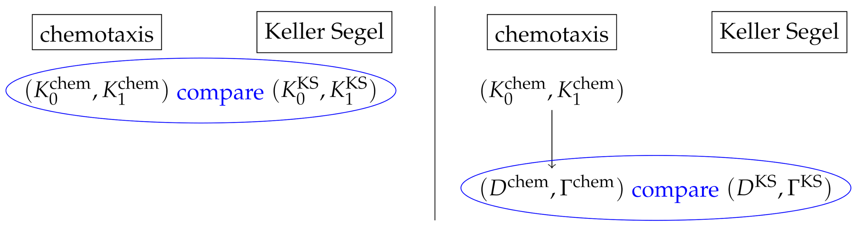
In order to reasonably compare the solutions to the inverse problems, the solutions have to be of the same kind. We choose to reconstruct $(K_0,K_1)$ in both the kinetic and macroscopic inverse problem; see Figure 1 (left). The macroscopic inverse problem is thus also formulated for $(K_0,K_1)$, which $(D,\Gamma )$ is a function of. Alternatively, one could also reconstruct $(D,\Gamma )$ from both models. In the kinetic setting, this would mean to reconstruct $(K_0^{\mathrm{chem}},K_1^{\mathrm{chem}})$ and then transform to values of $(D^{\mathrm{chem}},{\Gamma }^{\mathrm{chem}})$ by Equations (8) and (9); see Figure 1 (right).

We do not choose this alternative, because the information on the tumbling kernel $(K_0,K_1)$ is microscopic and thus more detailed. Furthermore, with a fixed $(K_0,K_1)$, $(D,\Gamma )$ can be uniquely determined, and thus the convergence can be viewed as a mere consequence; see also Remark 5.

Multiple experiments can be conducted using different initial profiles, but the same controlled $c(t,x)$ is used to ensure that the to-be-reconstructed $K_i$ is unchanged from experiment to experiment. Denoting by $k\in [1,\cdots ,K]$ the indices of the different initial data setups, and denoting by $j=(j_1,j_2)\in [1,\cdots ,J_1]\otimes [1,\cdots ,J_2]$ the indices of the measuring time and location, with $t_j=t_{j_1}$ being the measuring time, and ${\chi }_j={\chi }_{j_2}\in C_c\left({\mathbb{R}}^3\right)$ being the spatial test function, then, with (3) and (4) being the forward models, we take the measurements, respectively:

$$\begin{array}{ccc}\hfill {\mathcal{G}}_{jk}^{\epsilon ,\mathrm{chem}}(K_0,K_1)& ={\mathcal{M}}_j\left({\mathcal{A}}_{K_0,K_1}^{\epsilon }\left(f_0^{\left(k\right)}\right)\right)& ={\int }_{{\mathbb{R}}^3}{\int }_V{f}_{\epsilon }^{\left(k\right)}(x,t_j,v)dv{\chi }_j\left(x\right)dx,\hfill \end{array}$$

(14)

$$\begin{array}{ccc}\hfill {\mathcal{G}}_{jk}^{\mathrm{KS}}(K_0,K_1)& ={\mathcal{M}}_j\left({\mathcal{A}}_{K_0,K_1}^0\left({\rho }_0^{\left(k\right)}\right)\right)& ={\int }_{{\mathbb{R}}^3}{\rho }^{\left(k\right)}(x,t_j){\chi }_j\left(x\right)dx,\hfill \end{array}$$

(15)

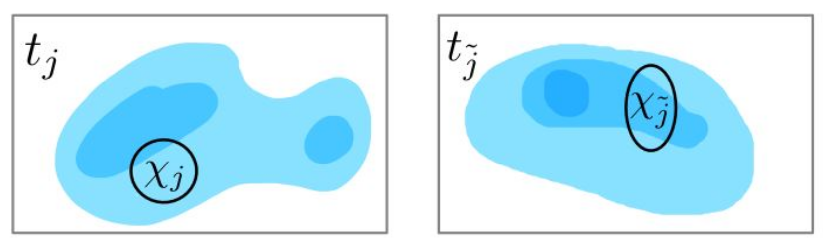
where ${\mathcal{M}}_j$ are the measuring operators with corresponding test functions $({\delta }_j,{\chi }_j)$. One can consider ${\chi }_j$ a compactly supported blob function concentrated at a certain location, meaning that all the bacterial cells in a small neighborhood are counted towards this particular measurement; see Figure 2. This is a reasonable model when counting bacteria in a small neighborhood or taking samples with a pipette.

Throughout the paper, we assume that the initial data and the measuring operators are controlled:

$$\begin{array}{cccc}\hfill & \parallel f_0^{\left(k\right)}{\parallel }_{L^1},{\parallel f_0^{\left(k\right)}\parallel }_{L^{\infty }}<C_{\rho },\hfill & \hfill & \forall k\hfill \\ \hfill & max\{\parallel {\chi }_j{\parallel }_{L_1},\parallel {\chi }_j{\parallel }_{L_2},\parallel {\chi }_j{\parallel }_{L_{\infty }},|\mathrm{supp}{\chi }_j{|}_{dx}\}<C_x,\hfill & \hfill & \forall j.\hfill \end{array}$$

(16)

Remark 4.

The measurements ${\mathcal{G}}_{jk}^{\epsilon ,\mathrm{chem}}(K_0,K_1),{\mathcal{G}}_{jk}^{\mathrm{KS}}(K_0,K_1)$ are formulated in a rather general form in Equations (14) and (15) due to the freedom in the choice of the test function ${\chi }_j\in C_c\left({\mathbb{R}}^3\right)$.

However, all subsequent derivations also hold true for the specific case of pointwise measurements with $t_j:=t_{j_1}$ and $x_j:=x_{j_2}$. The measurements would then be ${\mathcal{G}}_{jk}^{\epsilon ,\mathrm{chem}}(K_0,K_1)={\int }_V{f}_{\epsilon }^{\left(k\right)}(x_j,t_j,v)dv$ and ${\mathcal{G}}_{jk}^{\mathrm{KS}}(K_0,K_1)={\rho }^{\left(k\right)}(x_j,t_j)$, which would correspond to measuring operators ${\mathcal{M}}_j$ with test functions $({\delta }_{t_{j_1}},{\delta }_{x_{j_2}})$.

Since measuring error is not avoidable in the measuring process, we assume that it introduces an additive error and collect the data of the form

$$\begin{array}{ccc}\hfill y_{jk}^{\epsilon ,\mathrm{chem}}& =& {\mathcal{G}}_{jk}^{\epsilon ,\mathrm{chem}}(K_0,K_1)+{\eta }_{jk},\hfill \\ \hfill y_{jk}^{\mathrm{KS}}& =& {\mathcal{G}}_{jk}^{\mathrm{KS}}(K_0,K_1)+{\eta }_{jk},\hfill \end{array}$$

where the noise ${\eta }_{jk}$ is assumed to be a random variable independently drawn from a Gaussian distribution $N(0,{\gamma }^2)$ of known variance ${\gamma }^2>0$.

In the Bayesian form, the to-be-reconstructed parameter $(K_0,K_1)$ is assumed to be a random variable, and the goal is to reconstruct its distribution. Suppose a priori that we know that the parameter is drawn from the distribution ${\mu }_0$; then, the Bayesian posterior distributions for $(K_0,K_1)$ should be

$$\begin{array}{cc}\hfill {\mu }_{\epsilon ,\mathrm{chem}}^y(K_0,K_1)& =\frac{1}{Z^{\epsilon ,\mathrm{chem}}}{\mu }_{\epsilon ,\mathrm{chem}}^{(K_0,K_1)}\left(y\right){\mu }_0(K_0,K_1)\hfill \\ \hfill & =\frac{1}{Z^{\epsilon ,\mathrm{chem}}}{e}^{-\frac{1}{2{\gamma }^2}{\parallel {\mathcal{G}}^{\epsilon ,\mathrm{chem}}(K_0,K_1)-y\parallel }^2}{\mu }_0(K_0,K_1),\hfill \end{array}$$

(17)

using (3) as the forward model, and

$$\begin{array}{cc}\hfill {\mu }_{\mathrm{KS}}^y(K_0,K_1)& =\frac{1}{Z^{\mathrm{KS}}}{\mu }_{\mathrm{KS}}^{(K_0,K_1)}\left(y\right){\mu }_0(K_0,K_1)\hfill \\ \hfill & =\frac{1}{Z^{\mathrm{KS}}}{e}^{-\frac{1}{2{\gamma }^2}{\parallel {\mathcal{G}}^{\mathrm{KS}}(K_0,K_1)-y\parallel }^2}{\mu }_0(K_0,K_1),\hfill \end{array}$$

(18)

using (4) as the forward model. In the formula, $Z^{\circ }$ is the normalization constant to ensure $\int 1d{\mu }_{\circ }^y(K_0,K_1)=1$ and

$${\mu }_{\circ }^{(K_0,K_1)}\left(y\right)=e^{-\frac{1}{2{\gamma }^2}{\parallel {\mathcal{G}}^{\circ }(K_0,K_1)-y\parallel }^2}$$

is the likelihood of observing the data y from a model with a tumbling kernel or diffusion and drift term derived by $(K_0,K_1)$.

In Section 4, we specify the conditions on ${\mu }_0$ to ensure the well-definedness of ${\mu }_{\circ }^y$.

Remark 5.

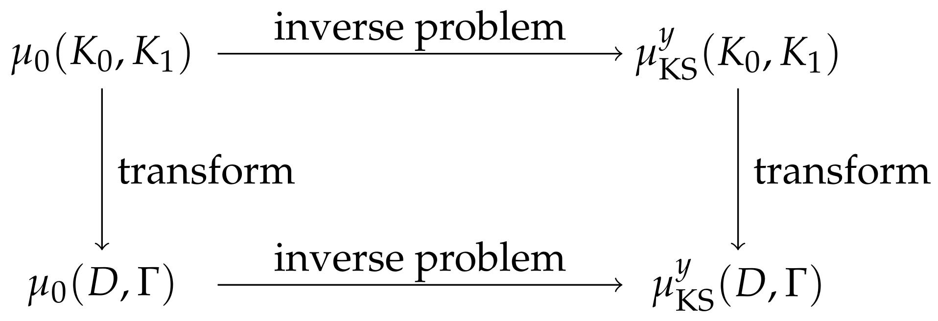
Since the macroscopic model does not explicitly depend on $(K_0,K_1)$, the distribution of ${\mu }_{\mathrm{KS}}^y(D,\Gamma )$ is of interest in the macroscopic description (4). There are two ways to derive it starting with a prior distribution on $(K_0,K_1)$: The natural way would be to transform the prior distribution to a prior on $(D,\Gamma )$ by Equations (8) and (9) and then consider the inverse problem of reconstructing $(D,\Gamma )$. This approach is displayed by the lower path in Figure 3. If, however, the posterior distribution ${\mu }_{\mathrm{KS}}^y(K_0,K_1)$ is calculated ahead of the transformation (as in our case), one could instead transform this posterior distribution directly to a distribution in the $(D,\Gamma )$ space following the upper path in Figure 3. Naturally, the question arises of whether the two ways lead to the same posterior distribution. It turns out that they do. Considering the second possibility, we see that the likelihood and thus the normalization constant only depend on $(D,\Gamma )$, because we are in the macroscopic model. Hence, only the prior distribution is transformed, as is the case for the first possibility.

4. Convergence of Posterior Distributions

One natural question arises. The two different forward models provide two different posterior distribution functions of $(K_0,K_1)$. Which distribution is the correct one, or, rather, what is the relation between the two posterior distributions?

As discussed in Section 2, the two forward models are asymptotically equivalent in the long-time large-space regime, so it is expected that the two posterior distributions converge as well. This suggests that the amount of information given by the measurements is equally presented by the two forward models. However, this convergence result is not as straightforward as it may seem. One issue comes from the control of initial data and the measurement operator. For each initial datum, the solution converges in $L^{\infty }\left([0,T];L_{+}^1\cap L^{\infty }({\mathbb{R}}^3\times V)\right)$; we now have a list of initial data, and the solutions are tested on a set of measuring operators, so we need a uniform convergence when tested on the dual space. Furthermore, to show the convergence of two distribution functions, a certain metric needs to be given on the probability function space. The issue of how the convergence for one set of fixed $(K_0,K_1)$ translates to the convergence on the entire admissible set also needs to be addressed.

By choosing the admissible set (6), we formulated an assumption on the tumbling kernels $(K_0,K_1)$ ahead of time. With this a priori knowledge, we showed the uniform boundedness and convergence of the solutions $f_{\epsilon }$ to the chemotaxis Equation (3) over the function set $\mathcal{A}$ in Theorem 1. This will play a crucial role in the convergence proof for the inverse problem. From here on, we assume that the prior distribution ${\mu }_0$ is supported on $\mathcal{A}$.

Before we show the convergence, as an a priori estimate, we first show the well-posedness of the Bayesian posterior distributions in Lemma 1, following [19,20].

Lemma 1.

If the initial conditions $f_0^{\left(k\right)}\in C_c^{1,+}({\mathbb{R}}^3\times V)$ and the test functions ${\chi }_j\in C_c\left({\mathbb{R}}^3\right)$ satisfy (16), then the following properties of the posterior distributions hold true:

(a) 

The measurements ${\mathcal{G}}^{\epsilon ,\mathrm{chem}}$ and ${\mathcal{G}}^{\mathrm{KS}}$ are uniformly bounded on $\mathcal{A}$ (and uniformly in ε).

(b) 

For small enough ε, the measurements ${\mathcal{G}}^{\epsilon ,\mathrm{chem}}$ and ${\mathcal{G}}^{\mathrm{KS}}$ are Lipschitz continuous with respect to the tumbling kernels $(K_0,K_1)$ under the norm $\parallel (K_0,K_1){\parallel }_{*}:=max(\parallel K_0{\parallel }_{\infty },\parallel K_1{\parallel }_{\infty })$ on $\mathcal{A}$.

(c) 

The posterior distributions are well-posed and absolutely continuous with regard to each other.

Proof.  

(a)

For every $(j,k)$, we have:

$$\begin{array}{ccc}\hfill |{\mathcal{G}}_{jk}^{\mathrm{KS}}(K_0,K_1)|& =& \left|{\int }_{{\mathbb{R}}^3}{\rho }^{\left(k\right)}(x,t_j){\chi }_j\left(x\right)dx\right|\hfill \\ & \le & \parallel {\chi }_j{\left(x\right)\parallel }_{\infty }\parallel {\rho }^{\left(k\right)}(·,t_j){\parallel }_{L^1\left({\mathbb{R}}^3\right)}=\parallel {\chi }_j\left(x\right){\parallel }_{\infty }{\parallel {\rho }_0^{\left(k\right)}\parallel }_{L^1\left({\mathbb{R}}^3\right)}\hfill \\ & \le & C_x{C}_{\rho }\hfill \end{array}$$

where we use the density conservation: ${\parallel \rho (·,t)\parallel }_{L^1\left({\mathbb{R}}^3\right)}={\parallel {\rho }_0\parallel }_{L^1\left({\mathbb{R}}^3\right)}$ for all t. Analogously, we have $|{\mathcal{G}}_{jk}^{\epsilon ,\mathrm{chem}}(K_0,K_1)|\le C_x{C}_{\rho }$. Note that this bound is independent of $\epsilon$.

(b)

For the chemotaxis model, we have for $(K_0,K_1),(\widetilde{K_0},\widetilde{K_1})\in \mathcal{A}$

$$\begin{array}{cc}\hfill |& {\mathcal{G}}_{jk}^{\epsilon ,\mathrm{chem}}(K_0,K_1)-{\mathcal{G}}_{jk}^{\epsilon ,\mathrm{chem}}(\widetilde{K_0},\widetilde{K_1})|=\left|{\int }_{{\mathbb{R}}^3}{\int }_V(f_{\epsilon }^{\left(k\right)}-{\tilde{f}}_{\epsilon }^{\left(k\right)})(x,t_j,v)dv{\chi }_j\left(x\right)dx\right|\hfill \\ \hfill & \le \parallel {\chi }_j{\parallel }_{\infty }{\int }_{\mathrm{supp}{\chi }_j}{\int }_V|{\overline{f}}_{\epsilon }^{\left(k\right)}(x,t_j,v)|dvdx\le C_x\left|V\right||\mathrm{supp}{\chi }_j{|}_{dx}{\parallel {\overline{f}}_{\epsilon }^{\left(k\right)}(·,t_j,·)\parallel }_{L^{\infty }({\mathbb{R}}^3\times V)}\hfill \\ \hfill & \le C_x^2\left|V\right|\parallel {\overline{f}}_{\epsilon }^{\left(k\right)}(·,t_j,·){\parallel }_{L^{\infty }({\mathbb{R}}^3\times V)},\hfill \end{array}$$

(19)

where $f_{\epsilon }^{\left(k\right)}$ and ${\tilde{f}}_{\epsilon }^{\left(k\right)}$ are solutions to the initial value problem (3) with initial condition $f_0^{\left(k\right)}$ and tumbling kernels $K_{\epsilon }=K_0+\epsilon K_1$ and ${\tilde{K}}_{\epsilon }={\tilde{K}}_0+\epsilon {\tilde{K}}_1$, respectively. Their difference ${\overline{f}}_{\epsilon }^{\left(k\right)}:=f_{\epsilon }^{\left(k\right)}-{\tilde{f}}_{\epsilon }^{\left(k\right)}$ satisfies the scaled difference equation:

$$\begin{array}{cc}\hfill {\epsilon }^2\frac{\partial }{\partial t}{\overline{f}}_{\epsilon }^{\left(k\right)}(x,t,v)+\epsilon v·& {\nabla }_x{\overline{f}}_{\epsilon }^{\left(k\right)}(x,t,v)={\tilde{\mathcal{K}}}_{\epsilon }\left({\overline{f}}_{\epsilon }^{\left(k\right)}\right)+{\overline{\mathcal{K}}}_{\epsilon }\left(f_{\epsilon }^{\left(k\right)}\right)\hfill \\ \hfill {\overline{f}}_{\epsilon }^{\left(k\right)}(x,0,v)& =0.\hfill \end{array}$$

Here, $\overline{\mathcal{K}}$ denotes the tumbling operator with kernel ${\overline{K}}_{\epsilon }:=K_{\epsilon }-{\tilde{K}}_{\epsilon }$. Integration in s at $(x-\frac{vs}{\epsilon },t-s,v)$ shows

$$\begin{array}{cccc}\hfill & {\overline{f}}_{\epsilon }^{\left(k\right)}(x,t,v)\hfill & \hfill ={\int }_0^t& {\tilde{\mathcal{K}}}_{\epsilon }\left({\overline{f}}_{\epsilon }^{\left(k\right)}\right)\left(x-\frac{vs}{\epsilon },v,t-s\right)+{\overline{\mathcal{K}}}_{\epsilon }\left(f_{\epsilon }^{\left(k\right)}\right)\left(x-\frac{vs}{\epsilon },v,t-s\right)ds\hfill \\ \hfill & \hfill & \hfill ={\int }_0^t& {\int }_V{\tilde{K}}_{\epsilon }{\overline{f}}_{\epsilon }^{\prime \left(k\right)}\left(x-\frac{vs}{\epsilon },v,v^{\prime },t-s\right)-{\tilde{K}}_{\epsilon }^{\prime }{\overline{f}}_{\epsilon }^{\left(k\right)}\left(x-\frac{vs}{\epsilon },v,v^{\prime },t-s\right)d{v}^{\prime }\hfill \\ \hfill & \hfill & \hfill +& {\int }_V{\overline{K}}_{\epsilon }{f}_{\epsilon }^{\prime \left(k\right)}\left(x-\frac{vs}{\epsilon },v,v^{\prime },t-s\right)-{\overline{K}}_{\epsilon }^{\prime }{f}_{\epsilon }^{\left(k\right)}\left(x-\frac{vs}{\epsilon },v,v^{\prime },t-s\right)d{v}^{\prime }ds.\hfill \end{array}$$

This yields

$$\begin{array}{cc}\hfill \parallel {\overline{f}}_{\epsilon }^{\left(k\right)}{(·,t,·)\parallel }_{L^{\infty }({\mathbb{R}}^3\times V)}\le & 2\parallel {\tilde{K}}_{\epsilon }{\parallel }_{\infty }\left|V\right|{\int }_0^t{\parallel {\overline{f}}_{\epsilon }^{\left(k\right)}(·,t-s,·)\parallel }_{L^{\infty }({\mathbb{R}}^3\times V)}ds\hfill \\ \hfill & +2\parallel K_{\epsilon }-\widetilde{K_{\epsilon }}{\parallel }_{\infty }\left|V\right|\parallel f_{\epsilon }^{\left(k\right)}{\parallel }_{\infty }t\hfill \\ \hfill \le & 4C\left|V\right|{\int }_0^t{\parallel {\overline{f}}_{\epsilon }^{\left(k\right)}(·,s,·)\parallel }_{L^{\infty }({\mathbb{R}}^3\times V)}ds\hfill \\ \hfill & +4\parallel (K_0-{\tilde{K}}_0,K_1-{\tilde{K}}_1){\parallel }_{*}\left|V\right|c_{f}T\hfill \end{array}$$

since one has $\parallel K_{\epsilon }{\parallel }_{\infty }\le 2{\parallel (K_0,K_1)\parallel }_{*}\le 2C$ for small enough $\epsilon <1$ and $f_{\epsilon }^{\left(k\right)}\le c_f$ is bounded in $L^{\infty }$ uniformly on $\mathcal{A}$ by Theorem 1 (a). Additionally, $c_f$ can be chosen to be independent of k by inserting the uniform boundedness of $\parallel f_0^{\left(k\right)}{\parallel }_{L^{\infty }}$ in (16) into Equation (12). The Grönwall lemma thus gives

$$\parallel {\overline{f}}_{\epsilon }^{\left(k\right)}{(·,t,·)\parallel }_{L^{\infty }({\mathbb{R}}^3\times V)}\le L(T,C,C_{\rho }){\parallel (K_0-{\tilde{K}}_0,K_1-{\tilde{K}}_1)\parallel }_{*}$$

with some coefficient L depending on T, C and $C_{\rho }$. Inserting this into Equation (19) results in the desired Lipschitz continuity.

We similarly study the Lipschitz continuity of the Keller–Segel measurements ${\mathcal{G}}_{jk}^{\mathrm{KS}}(K_0,K_1)$. The proof strategy is almost the same. With some computational effort, one can see:

$$\begin{array}{ccc}\hfill |{\mathcal{G}}_{jk}^{\mathrm{KS}}(K_0,K_1)& -& {\mathcal{G}}_{jk}^{\mathrm{KS}}({\tilde{K}}_0,{\tilde{K}}_1)|\le \parallel {\chi }_j{\parallel }_{L^2}{\parallel ({\rho }^{\left(k\right)}-{\tilde{\rho }}^{\left(k\right)})(·,t_j)\parallel }_{L^2}\hfill \\ & \le & C_{x}c(\parallel D-\tilde{D}{\parallel }_{L^{\infty }([0,T]\times {\mathbb{R}}^3;{\mathbb{R}}^{3\times 3})}+\parallel \Gamma -\tilde{\Gamma }{\parallel }_{L^{\infty }([0,T]\times {\mathbb{R}}^3;{\mathbb{R}}^3)})\hfill \end{array}$$

where $(\Gamma ,D),(\tilde{\Gamma },\tilde{D})$ are the drift and diffusion terms derived by the collision operators defined by $(K_0,K_1)$ and $({\tilde{K}}_0,{\tilde{K}}_1)$, respectively, by Equations (8) and (9). The constant c monotonously depends on the $L^2$ norms of ${\rho }^{\left(k\right)}$ and ${\nabla }_x{\rho }^{\left(k\right)}$, which are bounded uniformly on $\mathcal{A}$. By the linear relation between D and $\kappa$ and $\Gamma$ and $\theta$, this directly translates to

$$\begin{array}{cc}\hfill |{\mathcal{G}}_{jk}^{\mathrm{KS}}(K_0,K_1)-{\mathcal{G}}_{jk}^{\mathrm{KS}}({\tilde{K}}_0,{\tilde{K}}_1)|\le \tilde{c}c{C}_x(& \parallel \kappa -\tilde{\kappa }{\parallel }_{L^{\infty }([0,T]\times {\mathbb{R}}^3;L^2(V;\frac{dv}{F};{\mathbb{R}}^3))}\\ & +\parallel \theta -\tilde{\theta }{\parallel }_{L^{\infty }([0,T]\times {\mathbb{R}}^3;L^2(V;\frac{dv}{F}))}),\end{array}$$

with constant $\tilde{c}$ depending only on V. Finally, the Lax–Milgram theorem shows the continuous dependence of

$$\parallel \theta -\tilde{\theta }{\parallel }_{L^2(V;\frac{dv}{F})}+\parallel \kappa -\tilde{\kappa }{\parallel }_{L^2(V;\frac{dv}{F};{\mathbb{R}}^3)}\le \widehat{c}{\parallel (K_0,K_1)-({\tilde{K}}_0,{\tilde{K}}_1)\parallel }_{*}$$

where $\widehat{c}$ only depends on $V,\alpha ,C$.

(c)

By (a), the likelihoods $e^{-\frac{1}{2{\gamma }^2}{\parallel {\mathcal{G}}^{\circ }(K_0,K_1)-y\parallel }^2}$ are bounded away from zero and bounded uniformly on $\mathcal{A}$ (and in $\epsilon$). Thus, the normalization constants Z are too. Part (b) guarantees the measurability of the likelihoods. In total, this shows that the posterior distributions are well-defined and continuous with respect to each other. Since the likelihoods are continuous in y, the well-posedness of the posterior distributions is given.

□

We are now ready to show the convergence of the two posterior measures. There are two quantities that we use to measure the difference between two distributions:

• Kullback–Leibler divergence

  $$d_{\mathrm{KL}}({\mu }_1,{\mu }_2):={\int }_{\mathcal{A}}\left(log\frac{d{\mu }_1}{d{\mu }_2}\left(u\right)\right)d{\mu }_2\left(u\right)$$
• Hellinger metric

  $$d_{\mathrm{Hell}}{({\mu }_1,{\mu }_2)}^2=\frac{1}{2}{\int }_{\mathcal{A}}{\left(\sqrt{\frac{d{\mu }_1}{d{\mu }_0}\left(u\right)}-\sqrt{\frac{d{\mu }_2}{d{\mu }_0}\left(u\right)}\right)}^{2}d{\mu }_0\left(u\right).$$

The two metrics both evaluate the distance between the two probability measures ${\mu }_1$ and ${\mu }_2$, which are either absolutely continuous with respect to each other or with respect to a third probability measure ${\mu }_0$. Both are frequently used for comparing two distribution functions, e.g., in machine learning [25,26,27,28,29,30] or inverse problem settings [21,22]. Even though the Kullback–Leibler divergence lacks the symmetry and triangle-inequality properties of a metric, it has gained popularity due to its close connection to several information concepts, such as the Shannon entropy or the Fisher information metric [31]. Conversely, the Hellinger metric is a true metric. Although it does not have a demonstrative interpretation as does the Kullback–Leibler divergence, its strength lies in the fact that convergence in the Hellinger metric implies convergence of the expectation of any polynomially bounded function with respect to either of the posterior distributions, as explained in [19]. In particular, the mean, covariance and further moments of the distributions converge.

Before comparing the posterior measures, we need to have a look at the convergence of the measurements ${\mathcal{G}}^{\circ }(K_0,K_1)$.

Lemma 2.

Assuming that the initial and testing functions satisfy (16), the chemotaxis measurements ${\mathcal{G}}^{\epsilon ,\mathrm{chem}}$ converge to the Keller–Segel measurements ${\mathcal{G}}^{\mathrm{KS}}$ uniformly on $\mathcal{A}$ as $\epsilon \to 0$.

Proof. 

Theorem 1 shows the convergence of $f_{\epsilon }$ to $\rho F$ in $L^{\infty }([0,T],L_{+}^1\cap L^{\infty }({\mathbb{R}}^3\times V))$ uniformly on $\mathcal{A}$. As a consequence, we have the convergence of the measurements:

$$\begin{array}{ccc}& & \left|{\mathcal{G}}_{jk}^{\epsilon ,\mathrm{chem}}(K_0,K_1)-{\mathcal{G}}_{jk}^{\mathrm{KS}}(K_0,K_1)\right|\hfill \\ & =& \left|{\int }_{{\mathbb{R}}^3}{\int }_V{f}_{\epsilon }^{\left(k\right)}(x,t_j,v)dv{\chi }_j\left(x\right)dx-{\int }_{{\mathbb{R}}^3}{\rho }^{\left(k\right)}(x,t_j){\chi }_j\left(x\right)dx\right|\hfill \\ & \le & {\int }_{{\mathbb{R}}^3}{\int }_V|f_{\epsilon }^{\left(k\right)}(x,t_j,v)-{\rho }^{\left(k\right)}(x,t_j)F\left(v\right)\left|dv\right|{\chi }_j\left(x\right)|dx\hfill \\ & \le & \parallel f_{\epsilon }^{\left(k\right)}(·,t_j,·)-{\rho }^{\left(k\right)}(·,t_j){F\parallel }_{L^{\infty }({\mathbb{R}}^3\times V)}\left|V\right|\parallel {\chi }_j{\parallel }_{L^1\left({\mathbb{R}}^3\right)}\hfill \\ & \to & 0\hfill \end{array}$$

where we use the form $F=\frac{1}{V}$. By the uniform convergence of $f_{\epsilon }$ to $\rho F$, this holds uniformly on $\mathcal{A}$. Since the initial data and measuring test functions satisfy (16), we have the uniform convergence over $(j,k)$ as well. □

We can now prove the following theorem on the asymptotic equivalence of the two posterior measures describing the distribution of the tumbling kernels $(K_0,K_1)\in \mathcal{A}$ if the dynamics of the bacteria are modeled by the kinetic (3) or macroscopic Equation (4).

Theorem 2.

Let the measurement of the macroscopic bacteria density be of the form (14) and (15) for an underlying kinetic chemotaxis model or a Keller–Segel model, respectively. The measuring test functions ${\chi }_j\in C_c\left({\mathbb{R}}^3\right)$ and initial data $f_0^{\left(k\right)}\in C_c^{1,+}({\mathbb{R}}^3\times V)$ are assumed to satisfy (16). Given a prior distribution ${\mu }_0$ on $\mathcal{A}$ and an additive centered Gaussian noise in the data, the posterior distributions for the tumbling kernel derived from the kinetic chemotaxis equation and the macroscopic Keller–Segel equation as underlying models are asymptotically equivalent in the Kullback–Leibler divergence

$$\begin{array}{c}\hfill d_{\mathrm{KL}}({\mu }_{\epsilon ,\mathrm{chem}}^y,{\mu }_{\mathrm{KS}}^y)\stackrel{\epsilon \to 0}{\to }0.\end{array}$$

Proof of Theorem 2. 

With the above lemmas, one can proceed as in the proof in [21]. The integrand of the Kullback–Leibler divergence is by the definition of the normalization constants of order

$$\begin{array}{ccc}\hfill log\frac{d{\mu }_{\epsilon ,\mathrm{chem}}^y}{d{\mu }_{\mathrm{KS}}^y}(K_0,K_1)& =& log\left(\frac{{\mu }_0(K_0,K_1){\mu }_{\epsilon ,\mathrm{chem}}^{(K_0,K_1)}\left(y\right)}{Z^{\epsilon ,\mathrm{chem}}}\frac{Z^{\mathrm{KS}}}{{\mu }_0(K_0,K_1){\mu }_{\mathrm{KS}}^{(K_0,K_1)}\left(y\right)}\right)\hfill \\ & =& log\frac{Z^{\mathrm{KS}}}{Z^{\epsilon ,\mathrm{chem}}}+log\frac{{\mu }_{\epsilon ,\mathrm{chem}}^{(K_0,K_1)}\left(y\right)}{{\mu }_{\mathrm{KS}}^{(K_0,K_1)}\left(y\right)}\hfill \\ & =& \mathcal{O}\left(\right|Z^{\epsilon ,\mathrm{chem}}-Z^{\mathrm{KS}}\left|\right)+\mathcal{O}\left(\right|{\mu }_{\epsilon ,\mathrm{chem}}^{(K_0,K_1)}\left(y\right)-{\mu }_{\mathrm{KS}}^{(K_0,K_1)}\left(y\right)\left|\right)\hfill \\ & =& \mathcal{O}\left(\right|{\mu }_{\epsilon ,\mathrm{chem}}^{(K_0,K_1)}\left(y\right)-{\mu }_{\mathrm{KS}}^{(K_0,K_1)}\left(y\right)\left|\right).\hfill \end{array}$$

Thus, we estimate

$$\begin{array}{ccc}& & |{\mu }_{\epsilon ,\mathrm{chem}}^{(K_0,K_1)}\left(y\right)-{\mu }_{\mathrm{KS}}^{(K_0,K_1)}\left(y\right)|\hfill \\ & & =\left|exp\left(-\frac{\parallel y-{\mathcal{G}}^{\epsilon ,\mathrm{chem}}(K_0,K_1){\parallel }^2}{2{\gamma }^2}\right)-exp\left(-\frac{\parallel y-{\mathcal{G}}^{\mathrm{KS}}(K_0,K_1){\parallel }^2}{2{\gamma }^2}\right)\right|\hfill \\ & \le & c\left|\parallel y-{\mathcal{G}}^{\epsilon ,\mathrm{chem}}(K_0,K_1){\parallel }^2-{\parallel y-{\mathcal{G}}^{\mathrm{KS}}(K_0,K_1)\parallel }^2\right|\hfill \end{array}$$

for the Lipschitz constant $c<\infty$ of $exp(-\frac{\left|x\right|}{2{\gamma }^2})$ and

$$\begin{array}{cc}& \left|\parallel y-{\mathcal{G}}^{\epsilon ,\mathrm{chem}}(K_0,K_1){\parallel }^2-{\parallel y-{\mathcal{G}}^{\mathrm{KS}}(K_0,K_1)\parallel }^2\right|\hfill \\ & =\left|\mathrm{tr}\left[{\left(2y-{\mathcal{G}}^{\epsilon ,\mathrm{chem}}(K_0,K_1)-{\mathcal{G}}^{\mathrm{KS}}(K_0,K_1)\right)}^T\left({\mathcal{G}}^{\epsilon ,\mathrm{chem}}(K_0,K_1)-{\mathcal{G}}^{\mathrm{KS}}(K_0,K_1)\right)\right]\right|\hfill \\ & \le \parallel 2y-{\mathcal{G}}^{\epsilon ,\mathrm{chem}}(K_0,K_1)-{\mathcal{G}}^{\mathrm{KS}}(K_0,K_1)\parallel ·\parallel {\mathcal{G}}^{\epsilon ,\mathrm{chem}}(K_0,K_1)-{\mathcal{G}}^{\mathrm{KS}}(K_0,K_1)\parallel .\hfill \end{array}$$

The first factor is bounded uniformly on $\mathcal{A}$ and in $\epsilon$ by Lemma 1 (a) and Lemma 2 shows that the second factor converges to 0 uniformly on $\mathcal{A}$. It follows that

$$d_{\mathrm{KL}}({\mu }_{\epsilon ,\mathrm{chem}}^y,{\mu }_{\mathrm{KS}}^y)\to 0.$$

□

The boundedness of the the Hellinger metric by the Kullback–Leibler divergence

$$d_{\mathrm{Hell}}^2({\mu }_1,{\mu }_2)\le d_{\mathrm{KL}}({\mu }_1,{\mu }_2)$$

as shown in Lemma 2.4 in [32] together with Theorem 2 yields the asymptotic equivalence of the posterior distributions also in the Hellinger metric.

Corollary 1.

In the framework of Theorem 2, one has

$$\begin{array}{c}\hfill d_{\mathrm{Hell}}({\mu }_{\epsilon ,\mathrm{chem}}^y,{\mu }_{\mathrm{KS}}^y)\stackrel{\epsilon \to 0}{\to }0.\end{array}$$

5. Summary and Discussion

In this article, we considered bacterial movement in an environment with an attracting chemical substance that was not produced or consumed by the bacteria. The bacteria density was modeled to follow a chemotaxis Equation (3) on the kinetic level and a Keller–Segel Equation (4) on the macroscopic level. We studied the reconstruction of the tumbling coefficient using the measurement of the bacterial density at different times and locations using different initial data. After adapting the results from [5] in the parabolic scaling, we studied the equivalence between the reconstructions using the two different underlying models in the Bayesian framework. Assumptions on the prior information were made to guarantee the uniform convergence of the two forward models. This enabled us to show that the posterior distributions are properly defined and that convergence of the two posterior distributions holds true. The distance between two posterior distributions was measured in both the Kullback–Leibler divergence and the Hellinger metric.

The work presented here serves as a cornerstone of future research. On one hand, the study here can help in the design of an efficient inversion solver. Most inversion solvers are composed of many iterations of forward solvers. Since the kinetic chemotaxis equation lies on the phase space and is numerically much more expensive, the limiting Keller–Segel equation can serve as a good substitute for generating a good initial guess and speeding up the computation by reducing the number of iterations. On the other hand, the approach performed in this study is rather general, and with minor modification, it also provides the foundation for explaining experiments, such as [7].

References

- Patlak, C. Random Walk with Persistence and External Bias: A Mathematical Contribution to the Study of Orientation of Organisms. Bull. Math. Biophys. 1953, 15, 311–338. [Google Scholar] [CrossRef]
- Keller, E.F.; Segel, L.A. Model for chemotaxis. J. Theor. Biol. 1971, 30, 225–234. [Google Scholar] [CrossRef]
- Keller, E.F.; Segel, L.A. Traveling bands of chemotactic bacteria: A theoretical analysis. J. Theor. Biol. 1971, 30, 235–248. [Google Scholar] [CrossRef]
- Perthame, B. Transport Equations in Biology; Springer Science & Business Media: Berlin/Heidelberg, Germany, 2006. [Google Scholar]
- Chalub, F.; Markowich, P.; Perthame, B.; Schmeiser, C. Kinetic Models for Chemotaxis and their Drift-Diffusion Limits. Monatsh. Math. 2004, 142, 123–141. [Google Scholar] [CrossRef]
- Alt, W. Biased random walk models for chemotaxis and related diffusion approximations. J. Math. Biol. 1980, 9, 147–177. [Google Scholar] [CrossRef] [PubMed]
- Giometto, A.; Altermatt, F.; Maritan, A.; Stocker, R.; Rinaldo, A. Generalized receptor law governs phototaxis in the phytoplankton Euglena gracilis. Proc. Natl. Acad. Sci. USA 2015, 112, 7045–7050. [Google Scholar] [CrossRef] [Green Version]
- Keller, E.F.; Segel, L.A. Initiation of slime mold aggregation viewed as an instability. J. Theor. Biol. 1970, 26, 399–415. [Google Scholar] [CrossRef]
- Kowalczyk, R. Preventing blow-up in a chemotaxis model. J. Math. Anal. Appl. 2005, 305, 566–588. [Google Scholar] [CrossRef] [Green Version]
- Horstmann, D.; Winkler, M. Boundedness vs. blow-up in a chemotaxis system. J. Differ. Equ. 2005, 215, 52–107. [Google Scholar] [CrossRef] [Green Version]
- Perthame, B.; Vauchelet, N.; Wang, Z. The Flux Limited Keller-Segel System; Properties and Derivation from Kinetic Equations. Rev. Matemática Iberoam. 2019, 36, 357–386. [Google Scholar] [CrossRef] [Green Version]
- Erban, R.; Othmer, H. From Individual to Collective Behavior in Bacterial Chemotaxis. SIAM J. Appl. Math. 2004, 65, 361–391. [Google Scholar] [CrossRef] [Green Version]
- Si, G.; Wu, T.; Ouyang, Q.; Tu, Y. Pathway-Based Mean-Field Model for Escherichia coli Chemotaxis. Phys. Rev. Lett. 2012, 109, 048101. [Google Scholar] [CrossRef] [PubMed] [Green Version]
- Si, G.; Tang, M.; Yang, X. A Pathway-Based Mean-Field Model for E. coli Chemotaxis: Mathematical Derivation and Its Hyperbolic and Parabolic Limits. Multiscale Model. Simul. 2014, 12, 907–926. [Google Scholar] [CrossRef]
- Sun, W.; Tang, M. Macroscopic Limits of Pathway-Based Kinetic Models for E. coli Chemotaxis in Large Gradient Environments. Multiscale Model. Simul. 2016, 15, 797–826. [Google Scholar] [CrossRef] [Green Version]
- Perthame, B.; Sun, W.; Tang, M. The fractional diffusion limit of a kinetic model with biochemical pathway. Z. Angew. Math. Phys. 2017, 69, 1–15. [Google Scholar] [CrossRef] [Green Version]
- Othmer, H.; Hillen, T. The Diffusion Limit of Transport Equations II: Chemotaxis Equations. SIAM J. Appl. Math. 2002, 62, 1222–1250. [Google Scholar] [CrossRef] [Green Version]
- Othmer, H.; Dunbar, S.; Alt, W. Models of Dispersal in Biological Systems. J. Math. Biol. 1988, 26, 263–298. [Google Scholar] [CrossRef] [PubMed]
- Stuart, A.M. Inverse problems: A Bayesian perspective. Acta Numer. 2010, 19, 451–559. [Google Scholar] [CrossRef] [Green Version]
- Dashti, M.; Stuart, A. The Bayesian Approach to Inverse Problems. In Handbook of Uncertainty Quantification; Springer: Berlin/Heidelberg, Germany, 2015; pp. 1–118. [Google Scholar] [CrossRef] [Green Version]
- Newton, K.; Li, Q.; Stuart, A. Diffusive Optical Tomography in the Bayesian Framework. Multiscale Model. Simul. 2020, 18, 589–611. [Google Scholar] [CrossRef] [Green Version]
- Abdulle, A.; Blasio, A. A Bayesian Numerical Homogenization Method for Elliptic Multiscale Inverse Problems. SIAM/ASA J. Uncertain. Quantif. 2020, 8, 414–450. [Google Scholar] [CrossRef]
- Beal, J.; Farny, N.; Haddock-Angelli, T.; Vinoo Selvarajah, V.; Baldwin, G.S.; Buckley-Taylor, R.; Gershater, M.; Kiga, D.; Marken, J.; Sanchania, V.; et al. Robust estimation of bacterial cell count from optical density. Commun. Biol. 2020, 3, 1–29. [Google Scholar] [CrossRef]
- Hammes, F.; Egli, T. Cytometric methods for measuring bacteria in water: Advantages, pitfalls and applications. Anal. Bioanal. Chem. 2010, 397, 1083–1095. [Google Scholar] [CrossRef]
- Ran, Z.Y.; Hu, B.G. An identifying function approach for determining parameter structure of statistical learning machines. Neurocomputing 2015, 162, 209–217. [Google Scholar] [CrossRef]
- Clim, A.; Zota, R.D.; TinicĂ, G. The Kullback-Leibler Divergence Used in Machine Learning Algorithms for Health Care Applications and Hypertension Prediction: A Literature Review. Procedia Comput. Sci. 2018, 141, 448–453. [Google Scholar] [CrossRef]
- Hamadouche, A.; Kouadri, A.; Bakdi, A. A modified Kullback divergence for direct fault detection in large scale systems. J. Process. Control 2017, 59, 28–36. [Google Scholar] [CrossRef]
- Cieslak, D.; Hoens, T.; Chawla, N.; Kegelmeyer, W. Hellinger distance decision trees are robust and skew-insensitive. Data Min. Knowl. Discov. 2012, 24, 136–158. [Google Scholar] [CrossRef]
- Ni, X.; Härdle, W.K.; Xie, T. A Machine Learning Based Regulatory Risk Index for Cryptocurrencies. arXiv 2021, arXiv:2009.12121. [Google Scholar]
- Goldenberg, I.; Webb, G. Survey of distance measures for quantifying concept drift and shift in numeric data. Knowl. Inf. Syst. 2019, 60, 591–615. [Google Scholar] [CrossRef]
- Kullback, S.; Leibler, R.A. On Information and Sufficiency. Ann. Math. Stat. 1951, 22, 79–86. [Google Scholar] [CrossRef]
- Tsybakov, A.B. Introduction to Nonparametric Estimation, 1st ed.; Springer Series in Statistics: Berlin/Heidelberg, Germany, 2009. [Google Scholar] [CrossRef]
Figure 1.
Two ways to compare the inverse problems: determining and comparing the tumbling kernels for both underlying chemotaxis and Keller–Segel models (left) or determining the drift or diffusion coefficient for the Keller–Segel model and the tumbling kernel for the chemotaxis model and calculating the corresponding drift and diffusion coefficients.
Figure 2.
Measurement of the bacteria density (blue) at two different measuring times . The location of the test functions is indicated by the support in space of the test functions .
Figure 3.
Two ways to determine the posterior distribution from a prior on the tumbling kernels.
Publisher’s Note: MDPI stays neutral with regard to jurisdictional claims in published maps and institutional affiliations. |
© 2021 by the authors. Licensee MDPI, Basel, Switzerland. This article is an open access article distributed under the terms and conditions of the Creative Commons Attribution (CC BY) license (https://creativecommons.org/licenses/by/4.0/).
Share and Cite
MDPI and ACS Style
Hellmuth, K.; Klingenberg, C.; Li, Q.; Tang, M. Multiscale Convergence of the Inverse Problem for Chemotaxis in the Bayesian Setting. Computation 2021, 9, 119. https://0-doi-org.brum.beds.ac.uk/10.3390/computation9110119
AMA Style
Hellmuth K, Klingenberg C, Li Q, Tang M. Multiscale Convergence of the Inverse Problem for Chemotaxis in the Bayesian Setting. Computation. 2021; 9(11):119. https://0-doi-org.brum.beds.ac.uk/10.3390/computation9110119
Chicago/Turabian StyleHellmuth, Kathrin, Christian Klingenberg, Qin Li, and Min Tang. 2021. "Multiscale Convergence of the Inverse Problem for Chemotaxis in the Bayesian Setting" Computation 9, no. 11: 119. https://0-doi-org.brum.beds.ac.uk/10.3390/computation9110119
Note that from the first issue of 2016, this journal uses article numbers instead of page numbers. See further details here.