Simulation and Analysis of Self-Replicating Robot Decision-Making Systems

Department of Computer Science, North Dakota State University, Fargo, ND 58108, USA
*
Author to whom correspondence should be addressed.
Computers 2021, 10(1), 9; https://0-doi-org.brum.beds.ac.uk/10.3390/computers10010009
Submission received: 13 December 2020
/
Revised: 31 December 2020
/
Accepted: 1 January 2021
/
Published: 6 January 2021
(This article belongs to the Special Issue Feature Paper in Computers)
Abstract
:Self-replicating robot systems (SRRSs) are a new prospective paradigm for robotic exploration. They can potentially facilitate lower mission costs and enhance mission capabilities by allowing some materials, which are needed for robotic system construction, to be collected in situ and used for robot fabrication. The use of a self-replicating robot system can potentially lower risk aversion, due to the ability to potentially replenish lost or damaged robots, and may increase the likelihood of mission success. This paper proposes and compares system configurations of an SRRS. A simulation system was designed and is used to model how an SRRS performs based on its system configuration, attributes, and operating environment. Experiments were conducted using this simulation and the results are presented.
1. Introduction
The concept of self-replicating robots has been around for some time—dating back to the 1940s and earlier [1]. With the advent of 3D printing technology, the development of self-replicating robots is more feasible to implement than it was previously. This opens the door to research and development opportunities in this area of robotics.
Self-replicating robots can be beneficial for use in areas that are difficult for humans to access or where it is prohibitive to bring in materials and supplies. Though these may be the primary areas of benefit, this type of robot system could also be used in a wide variety of other applications. One application domain that may especially benefit from self-replicating robots is aerospace. Launching materials into space can be prohibitively expensive, which may drive a need for utilizing in-situ materials [2].
This paper focuses on system configurations for self-replicating robot systems (SRRSs). A challenge of analyzing self-replicating robot systems, and the decision-making algorithms for those systems, is that there is not currently a standard means to simulate these systems. For this purpose, a simulation was developed to provide a means to implement, assess and compare system configurations and autonomous decision-making algorithms for SRRSs. The simulation system is based on work discussed previously in [3,4]. The proposed simulation system focuses on the decision-making and planning of the system as opposed to modeling the physics of self-replication. An experiment was conducted using this simulation system, and the results are presented.
The work presented herein proposes a categorization for self-replicating robot systems and compares the proposed categories (system configurations) using the proposed simulation approach. The proposed simulation approach is used with parameters that may fit mission constraints in order to inform the decision of how an SRRS should be configured and commanded. Furthermore, the results from the simulated experiment can be utilized as heuristics which may aid in determining which types of buildable robots may be needed for a particular mission or objective. For example, the initial resources provided to the system may influence the rate at which different system configurations can expand. A system’s initial configuration could be adjusted based on analysis of the results presented herein in order to optimize the system to fulfill objective-related requirements.
The remainder of this paper is organized as follows: First, in Section 2, relevant background information is outlined. Second, in Section 3, a proposed replication categorization is discussed. Third, in Section 4, a simulation that is used to model self-replicating robot systems is detailed. Then, an experiment is conducted (in Section 5) which utilizes this simulation model and the data and analysis from those simulations is presented (in Section 6 and Section 7), before concluding.
2. Background and Related Work
This section reviews relevant prior work, in several areas, that provides a foundation for the work presented herein. First, prior work on self-replicating robots is reviewed. Next, the additive manufacturing research that facilitates the self-replication of the robots is discussed. Third, techniques for robot foraging are presented.
2.1. Self-Replicating Robots
Research in the field of self-replicating robots largely originated with work performed by von Neumann [5,6]. In particular, his work developed the logical foundations of self-replication and theoretical machines such as a universal assembler and cellular automaton [1,5]. More recently, the technology to actually perform self-replication has become feasible. Beuchat and Haenni [7], for example, created a hardware implementation of cellular automaton and published the results of its analysis in 2000. Suthakorn, Kwon, and Chirikjian [6] demonstrated the operations of a semi-autonomous robot, made from LEGO Mindstorm kit parts, that performs supervised replication.
More practically, the RepRap 3D printer [8] has been used as a template for the creation of numerous consumer-grade 3D printers, with an emphasis on the use of 3D-printed parts. Thus, once a user has a working RepRap printer, it is possible to produce many of the mechanical parts required to make another RepRap printer. However, unlike the SRRSs discussed herein, which use autonomous replication, RepRap construction requires significant human involvement.
2.2. Additive Manufacturing
Additive manufacturing (AM) is a process of joining materials to make objects from 3D model data, usually by applying layer upon layer of material [9,10]. AM methodologies, such as 3D printing, have been used for various commercial purposes. These application areas include fabricating prototypes, replacement parts, automobile components, aircraft components, robotic components, hearing aid molds, dental crowns, eyeglass frames, and prosthetic limbs [11,12,13].
A common AM method, widely used in modern commercial 3D printing, is fused deposition modeling (FDM) [9]. This method involves extruding polymer through heated nozzles to create a part [14]. Various other AM methods are used for a variety of applications, including the use of an ultraviolet laser to harden a photosensitive polymer (stereolithography), and using a laser to selectively melt metal or polymeric powder (laser sintering) [11].
Creating robots using 3D printing is well established and numerous robots and robot parts have been created using 3D printing [3]. The MU-L8 robot [15], for example, utilized 3D-printed limbs to emulate human movements and play robot soccer. For more distant applications, the use of in-situ resources is necessary to prolong mission duration and, potentially, facilitates having a greater ability to take risks [3]. Examples of in-situ resources being proposed for 3D printing include the use of basalt printing of structures for Martian exploration [16]. The use of a D-shape printer for building infrastructure out of regolith on the Earth’s moon [17] and the use of a collection of simple self-replicating robots to exploit lunar material and energy resources [18] have also been previously considered.
2.3. Robot Foraging
Robot foraging is broadly defined as robots searching for and collecting objects and subsequently bringing them to a collection point [19]. This can be divided into multiple separate stages, such as the problem of recognizing resources and the problem of collecting them [3].
Recognizing resources in a given environment can be accomplished in many ways. For example, reflection seismology (which is similar in concept to radar) has been used to discover oil and natural gas [20]. Robotic visual recognition of surface resources can be accomplished by processing images using trained deep convolutional neural networks [21] and other machine vision techniques. The foregoing techniques could identify many of the resources required for robot replication. Additional techniques may be needed for robots with additional mission-specific resource identification needs.
Once the needed resources are identified, the robots must be able to autonomously collect them [3]. A number of prior studies demonstrate relevant capabilities. For example, Green and Vogt [22] proposed a multi-robot system that could cooperatively and autonomously mine ore using rock drills. Similarly, Shaffer and Stentz [23] tested a robotic system for coal mining that could autonomously navigate and reposition itself underground using a laser range finder. Dunker et al. [24] demonstrated a proof of concept for utilizing teams of robots that could automatically gather regolith on the surface of the Moon with an actuated scoop. It would then bring the collected materials to a central processing station.
3. Proposed Replication Categorization
In this subsection, the categorization scheme utilized for the simulation and experimentation is detailed. There are many attributes that could be used to characterize an overall replication scheme. For instance, whether multiple robots need to be involved in making a new robot or if the hardware/design evolves over time [25] are both possible criteria. However, the categorization approach used for this work is to categorize the system based on what types of robots the system can build and which of those types have a replication-related capability. This (replication-related capability) means a capability used for fabricating, building, or assembling parts for a new robot.
The utilized categorization consists of a combination of two separate classifications. The first classification, the replication approach, consists of centralized, decentralized, and hierarchical. The second classification, the production approach, consists of heterogeneous and homogeneous.
3.1. Centralized Replication Approach
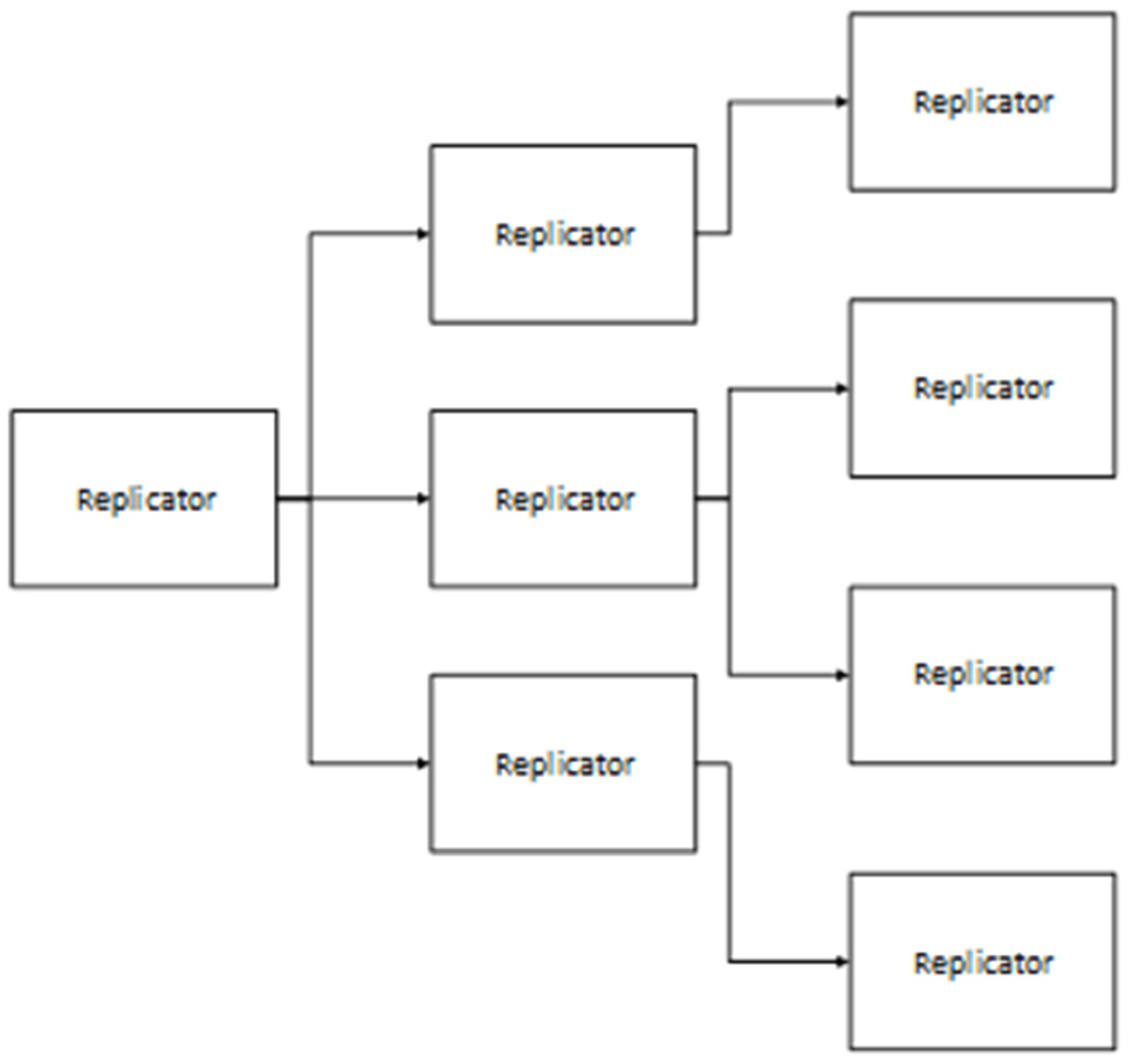
With the centralized replication approach, robots that have a replication-related capability are not buildable by the robot system itself. Initial or factory-made robots are solely used for replication related capabilities. A replicator robot is set up and acts as a replication center, as depicted in Figure 1. It is able to build robots that do not have replication-related capabilities that can collect resources or accomplish other goals.
Having a central node dedicated to the replication process has benefits and drawbacks. One benefit to this approach is that the regular robots (produced by the central node) do not have to have the replication equipment installed, allowing the otherwise consumed materials to be used for other purposes (i.e., it reduces material usage). However, a key drawback to this approach is that if the central replicator node malfunctions, it is a central point of system failure [3].
Another benefit, for some applications, is that all of the replication-related materials collected are brought to a centralized stockpile. This prevents the replication process from getting bottlenecked by poor resource exchange between robots (although this could be potentially remedied by the implementation of a cooperation scheme in non-centralized systems) [3]. However, the requirement to bring all replication resources to the central node also presents drawbacks. This is particularly problematic when the resources needed for robotic production and the location needing the robots produced from these resources are located far away from the central production location.
3.2. Decentralized Replication Approach
The decentralized replication approach, which is depicted in Figure 2, includes replication capabilities in all of the robots in the robot system. A benefit to this approach is that, in the event of a catastrophic event, if one robot survives and has replication resources available, it could potentially make more robots to repopulate the system. This capability leads to increased survivability of the multi-robot system [3]. It may also allow the multi-robot system to split into multiple groups that do not have a dependency on a central hub (as they would in the centralized configuration). A drawback to this approach is that each robot needs to include replication equipment, which may be rare or specialized equipment. Even if it does not require rare resources or equipment, the approach is likely to require additional standard resources. Another potential drawback is that a specialized replicator robot could potentially be made with higher quality equipment, which may make it more versatile in transforming raw materials into new robots or result in higher quality being produced. Not having the ability to use a wide array of raw materials may cause problems in certain environments.
3.3. Hierarchical Replication Approach
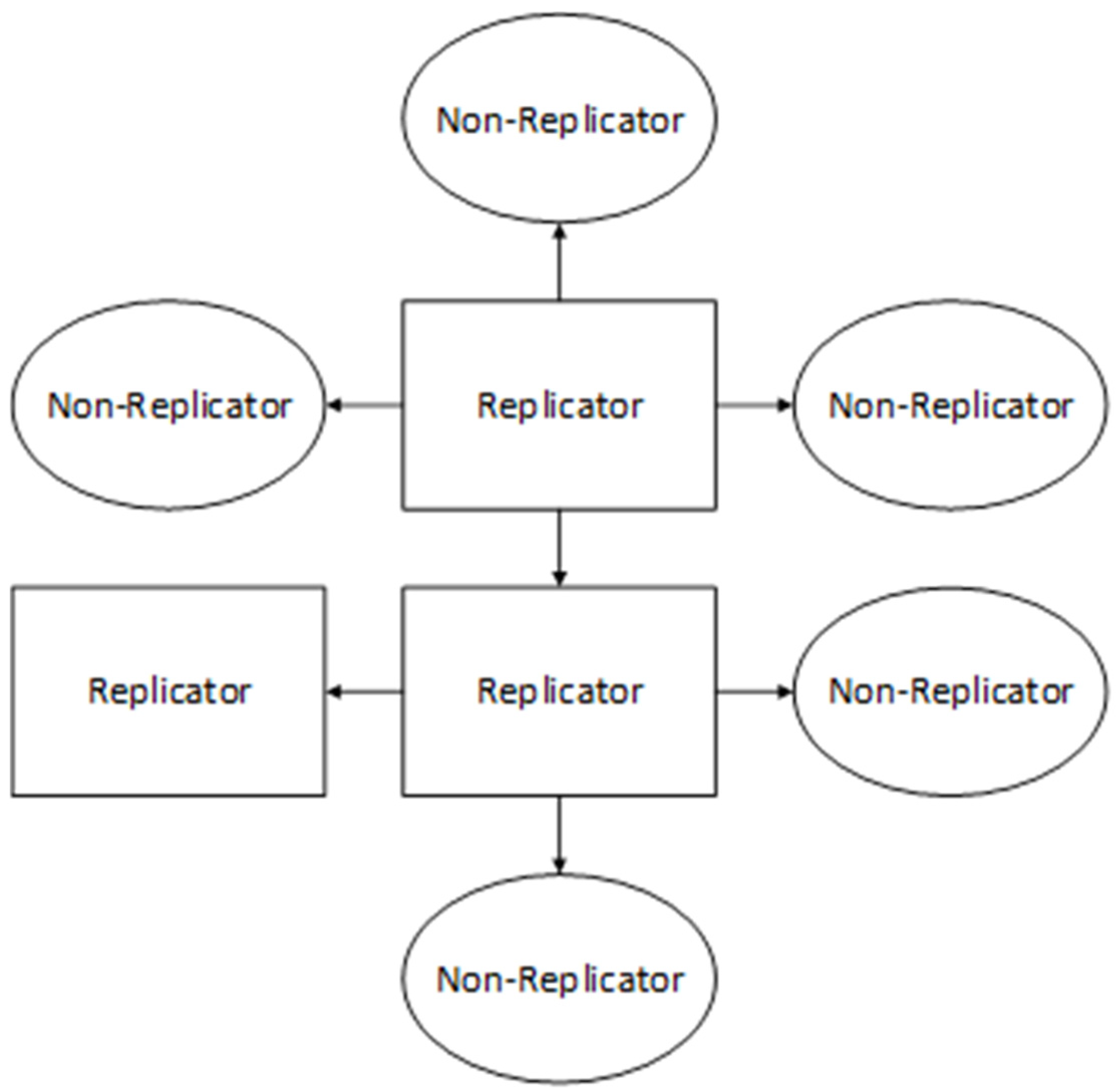
The hierarchical replication approach, which is depicted in Figure 3, is a combination of the centralized and decentralized approaches. Systems of this type are capable of building robots with replication-related capabilities as well as robots without these capabilities. The benefits and drawbacks of this approach are dependent on the ratio of robots with replication-related capabilities to non-replicating robots. At the extremes, the benefits and drawbacks approximate those of the centralized or decentralized approach.
3.4. Production Approach: Homogeneous or Heterogeneous
The production approach categorization is made in addition to (and is distinct from) the replication approach categorization. The production approach consists of two classifications, homogeneous and heterogeneous. For multi-robot systems, in general, a homogeneous system is composed of robots that are all of the same design, while having multiple types of robots makes the system heterogeneous [26]. Under the replication classification scheme used herein, the characterization of a multi-robot system as homogeneous or heterogeneous, in terms of replication, is as follows: the homogeneous production approach means that the system uses a single robot type that has all of the necessary replication-related capabilities. In contrast, the heterogeneous production approach means that the system uses two or more robot types that have replication-related capabilities. The replication-related capabilities used across the robot types used in the system must be partially independent of each other to qualify for this classification.
The benefits of a homogeneous system include the potential reduction in task allocation complexity, as only one robot is needed for replication tasks. This approach may also increase the survivability of the system as a single surviving robot could repopulate the robot system (given sufficient resources and time).
The benefits of a heterogeneous system include resource savings. Using the minimum amount of materials required to produce a functional robot—meeting relevant quality standards—is desirable. The heterogeneous approach allows the greatest number of robots possible to be constructed, given the available level of in-situ collected and stored materials. Tailoring robots to specific roles ensures that each robot only includes the necessary functionality, saving resources [27]. Another consideration is the selection of a design that makes use of resources that are available and abundant [3]. Choosing a design that utilizes locally abundant resources maximizes the number of robots that can be produced. A homogeneous approach would preclude this type of adaptation.
3.5. Conceptual Example
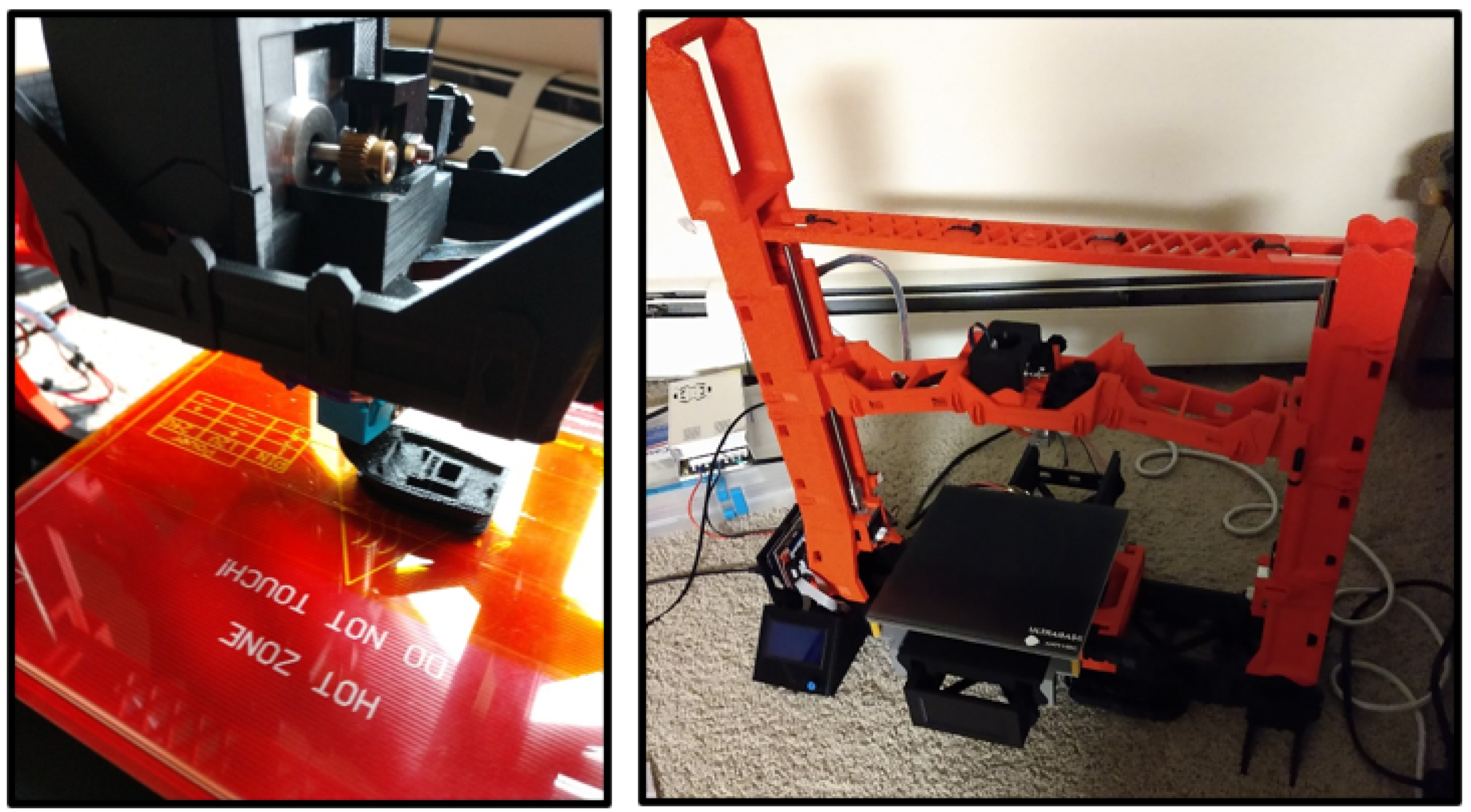
A conceptual example robot system, a largely 3D-printed 3D printer, was built and is depicted in Figure 4. Its design is a slightly modified version of the “Snappy” RepRap [28]. Its frame is 3D printed and “snaps” together using the mechanical design of the printed components. The nonprintable components include stepper motors (for moving parts), a heating block and an extruder, a heated print bed (for print adherence), and control electronics. It is capable of 3D printing components that could be used to assemble additional 3D printers or robots. However, the prototype system does not include an automated assembly capability.
In addition, a small (mostly) 3D-printed robot was constructed (which is depicted in Figure 5) and programmed with software that allows it to perform simple resource location tasks (e.g., find a colored spool of 3D printer filament). This small 3D-printed robot is meant to compliment the 3D-printed 3D printer for the purposes of the example implementation. The prototype does not have the capability to manipulate and move any located filament in its current design. It consists of a 3D-printed chassis and 3D-printed tracks, which are driven by two servo motors (based on design from [29]). Its on-board computer is a Nvidia Jetson Nano, which processes the visual data from the Zed Mini stereo-camera in order to perform simple resource identification and localization. It is powered by a rechargeable lithium-ion battery pack that fits within the chassis.
The conceptual prototype models are intended to illustrate a simplistic example SRRS system. For the experiment discussed in the subsequent sections, a hypothetical SRRS system that has more uniform robot models is utilized. For example, the size of the non-replicating robot would be more comparable to the 3D print-capable robot and a comparable amount of filament (raw printing materials) would be used.
4. Proposed Simulation System
In this section, the operations of the proposed simulation system are detailed. The system consists of an SRRS command system interacting with an environmental simulator. The simulation system was designed to facilitate experimentation to further understand the constraints and variables involved in SRRS configuration decisions and robotic command decision-making strategies.
A simulation run is divided into a number of iterations (called time-steps). The number of time-steps for a given run is determined by user input. Each time-step corresponds to a block of time, with the simulation starting at time-step zero and progressing until the desired number of time-steps is reached (where each time-step corresponds with one iteration). In each time-step of the simulation, SRRS-simulated robots perform tasks which involve acquiring resources, converting resources, or assembling new robots. The following sections describe these in more detail, along with the operations of the simulation from a wholistic standpoint.
4.1. Resources and Task Types
There are three different types of resources in the simulation system, which were proposed in previous work [3,4]. These resource types are as follows:
- Nonprintable components: components that the robot system does not have the capability to print (or otherwise make in-situ), such as control units (processors) and motors.
- Printable components: components that are fabricated by the robot system during the simulation, such as frames and other structural elements for new robots.
- Raw printing materials: materials that are used in the printing process. The printing process would yield the printable component resource type, so the raw material type requires a fabricating step before materials are useable (as components) to build new robots.
The robot system begins the simulation with an initial defined amount of each of these resource types (listed in Table 1). The environment also has a certain amount of raw printing material available that robots can collect.
For the purposes of the simulation, each of these component types are represented by a single numerical quantity. The nonprintable components are combined into a single numerical quantity which refers to a volume (or mass) of components. In practice, the nonprintable components would include a diverse range of parts that would not be interchangeable with one another (i.e., motors, processors or cables) but which would be constrained by the same mass and volume limitations. A simulation could be run beforehand and used to project which nonprintable components would need to be stored in that allotted volume. For the printable component resource type, the components are assumed to be interchangeable for simplicity, although in practice a system would be needed to decide what specific type of printable components should be fabricated. The printable component resource type is related to the raw printing material resource type in volume, where the raw material conversion to printable components in the simulation is determined by the Print_Efficiency parameter.
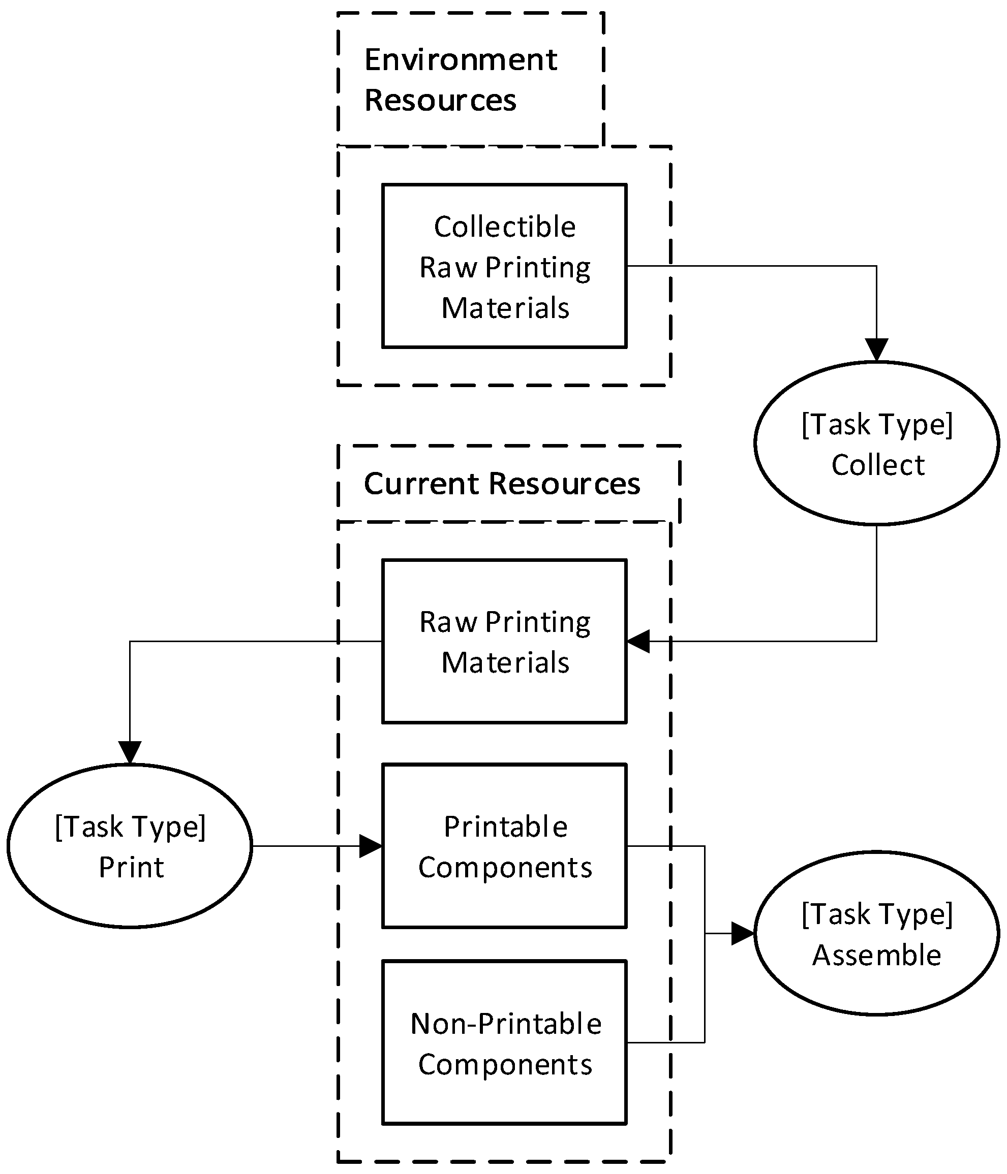
There are four task types in the simulation: three which perform an action (depicted in Figure 6) and one which represents a default state indicating that a robot is currently performing no action (idle). The descriptions of the task types are as follows:
- Collect: a task type where the robot gathers raw printing materials from the environment and adds the gathered materials to the robot system’s inventory. This task type has a time-step duration of 1, meaning that if a robot is assigned to perform this task type it would complete it in a single time-step. Upon completion of this task, raw printing materials are removed from the environment and added to the robot system’s resource pool. The amount collected upon completion is a parameter (Collect_Amount), which represents an average amount returned per time-step (as it would vary based on resource sparsity).
- Print: a task type where the robot takes raw printing materials and fabricates them into printable components. This task type has a time-step duration of 1, meaning that if a robot is assigned this task type it would complete it in a single time-step. Upon completion of this task, raw printing materials are removed (Print_Amount) from the robot system’s resource pool and printable components are added to the robot system’s resource pool. This represents an average amount of components printed per time-step (including an allowance for failed prints). The conversion factor of raw printing materials to printable components is represented by the parameter Print_Efficiency.
- Assemble: a task type where the robot takes nonprintable components and printable components from the robot system’s resource pool and assembles them into a new robot. This task type has a duration that varies by the robot type being assembled. Upon completion of this task, the newly assembled robot is added to the robot system.
- Idle: a default task type which is assigned to any robot not performing any other action during a time-step. This task type has no associated duration, because it does not have any completion actions/events.
4.2. Robot Types
In the simulation, there are four types of robots: normal, printer, assembler, and replicator. In each time-step, each robot is either idle, gathering resources, printing components, or assembling a new robot. However, certain robot types are restricted in what types of tasks they can perform. These restrictions are listed in Table 2. All robot types are capable of being idle. Not all types of robots must be included in any given simulation run.
The robots in the simulation are considered single-task (ST) robots that carry out single-robot (SR) tasks with a time-extended assignment (TA). Thus, the robot systems in the simulation would be categorized as ST-SR-TA according to the task allocation taxonomy proposed by Gerkey in [30].
The material cost of each robot type is directly related to its capabilities. Capability costs for each included capability are added together to determine the cost of the robot type. For example, the normal robot type cost is just the base cost, while the printer robot type’s cost is calculated by adding the base cost plus the printing capability cost. This work assumes that the robot design for each robot type is similar and the added cost per additional capability would be the cost of upgrading the normal robot type to have that additional capability. The default values (i.e., initial parameter values) for these costs are listed in Table 3. These values are simulation parameters and can be adjusted from run to run of the simulation, to define the experimental conditions that are being studied by each simulation run. For example, the 3D-printed 3D printer described in Section 3.5 requires approximately 3.1 kg of PLA filament and approximately 1.64 kg of nonprintable components (stepper motors, heated print bed, and control electronics) [28]. In this example, the ratio of printable component mass to nonprintable component mass is 2 to 1. This is just one example and the units of the simulation are not set, but rather represent ratios of resources.
In an aerospace application, a mission might use an SRRS to print a larger structure (such as a habitat) and a number of 3D print-capable robots would thus be needed. The Curiosity rover has an estimated mass of over 900 kg [31], and contour crafting 3D printers (for constructing aerospace habitats) can have masses of approximately 500 kg [32]. Although these robots are not themselves 3D printed (and there currently are no standardized designs for 3D-printed aerospace robots), the differences in mass illustrate the significant variability that could exist between potential SRRS implementations. In this case, these values would differ from the default values in Table 3, where it is by default equal. However, these parameters are set at different levels from the default values in the experimental conditions discussed in subsequent sections.
The work presented herein assumes that the design of each robot type is fixed during each simulation run and does not incorporate any design changes over the course of the run. The simulation system presented herein could be updated, in future work, to model systems that incorporate during-run robot upgrades as well as to consider the trade-offs presented by the use of evolutionary algorithms [33] and evolvable hardware [34]. All three of these robotic system advancements present cost versus benefit tradeoffs that can be analyzed similarly to the ones considered in the current work.
4.3. Robot Build Quality
An important capability of a self-replicating robot system is the ability to fabricate parts and assemble new robots. This introduces the question of the quality of the built robot, as a robot built in-situ may have quality defects (without the ability to simply discard it with minimal impact, such as in a factory setting). To facilitate assessment, the simulation assigns each robot a build quality. A robot’s build quality value ranges from zero to one, with one being very high quality and zero being very poor quality. The quality value is a decimal value (not a binary one).
The build quality value is determined as follows. When a new robot is built, it has a build quality value determined based on the robot that assembled it. First, a random value is generated, and if the value is above one minus the increase quality chance, then the newly assembled robot’s build quality equals the build quality of the assembling robot plus a random number between the increase quality lower and upper bound parameter values (zero and one are a strictly enforced minimum and maximum). If not within the increase chance, then it is compared to the decrease quality chance parameter. Similar to before, if the random number is below the decrease quality chance then the newly assembled robot’s build quality equals its builder’s quality minus a random number between the upper and lower bounds. The pseudocode for this process is shown in Equation (1). The variable RobotQuality refers to the build quality of the newly constructed robot; AssemblerQuality refers to the build quality of the robot that assembled it.
4.4. Task Risks
Tasks have a risk of failing in a manner which harms or destroys the robot performing the task. The risk amount values are adjustable parameters. In the simulation system, the particular consequence of each task type is as follows. Collecting resources involves robots foraging in an environment. This puts them at risk of being stuck, trapped, navigationally lost, or otherwise lost due to environmental hazards. This is not the case with printing or assembling, as navigating the environment is not part of these tasks. The printing task has a potential consequence of the robot’s printing capabilities being lost due to a significant hardware malfunction occurring. Similarly, the assemble task has the potential consequence of the assembly hardware breaking down. The default risk amounts were chosen based on estimations but would likely vary significantly based on hardware specifications and environmental factors. These are configurable parameters within the simulation system, to facilitate experimentation.
The build quality of the robot performing a task may also affect the associated risks of performing a given task. The rationale behind this is that as the quality of a robot decreases, the risk of it encountering problems performing a task would likely increase. Equation (2) was utilized in order to represent this.
In Equation (2), a robot’s lack of quality increases the risk in a manner related to the task type’s risk. Omitting RiskTask_Type in the multiplication would increase the risk by a constant, which could end up being a dominant factor and negate the relevance of the task’s inherit risk. A risk modifier parameter (RiskQuality_Modifier) is then applied in order to add a weighting factor for the impact of quality on the risk.
Another consideration is that the initial robots of the robot system would likely be factory built and tested to a high degree. Thus, the associated risk amount of these (likely thoroughly tested) initial factory-built robots would be less than robots built by the robot system. In this regard, a parameter (RiskFactory_Modifier) is used to scale the risk cost of factory-built robots performing a task.
The simulation system, by design, does not model the potential for general robotic failure that is unrelated to production processes, task performance and defects, as this would effectively be an arbitrary noise value for the analysis presented herein. System developers that have specific projected failure rates—particularly if the incidental failure rate was expected to be a significant factor in system operations—should consider this in modeling specific operations in specific environments. Adding this capability to the simulation system is a topic for potential future work.
4.5. Self-Replicating Robot System Configurations
In this subsection, the configurations of SRRSs used for the experiments reported on in this paper are presented. These configurations are based off the categorization discussed in Section 3. The replication system configurations are a combination of choices from two sets. The first set, the replication approach, consists of centralized, decentralized, and hierarchical. This determines how many robots have a replication-related capability. The replication-related capabilities, for this simulation, include the assembly and print task types. The normal type robots are therefore considered not to have a replication related capability in this simulation (due to not having the assembly or print capability).
The second set, the production approach, consists of homogeneous and heterogeneous. This determines whether a single type of robot is used for all replication activities or if there are multiple types of replication-capable robots. The choices from each set are combined to derive the replication system configurations that are possible. The configurations are as follows:
- Centralized homogeneous (CHO): One robot is responsible for both printing components and assembling them. Constructed robots are of the normal type and either gather resources or complete other objectives.
- Decentralized homogeneous (DHO): All robots have the capability to print components, assemble them, and gather resources or complete other objectives.
- Hierarchical homogeneous (HHO): There are a variable number of robots capable of printing components and assembling them. There are also a variable number of normal type robots.
- Centralized heterogeneous (CHE): One robot is responsible for printing components, and another (distinct) robot is responsible for assembling them. Constructed robots are of the normal type and either gather resources or complete other objectives.
- Decentralized heterogeneous (DHE): Robots have either the capability to print components or the capability to assemble them. All robots can gather resources or complete other objectives.
- Hierarchical heterogeneous (HHE): There are a variable number of robots capable of printing components, a variable number capable of assembling them (distinct from printing group), and a variable number of normal type robots. All robots can gather resources or complete other objectives.
A robot completing other objectives would correspond with the robot completing mission objectives, if any are specified. However, the completion of other objectives is not performed in the experiment in this paper.
For the purposes of the simulation, the homogeneous configurations start with a single replicator robot, while heterogeneous configurations start with two robots: an assembler robot and a printer robot.
4.6. Simulation Operations
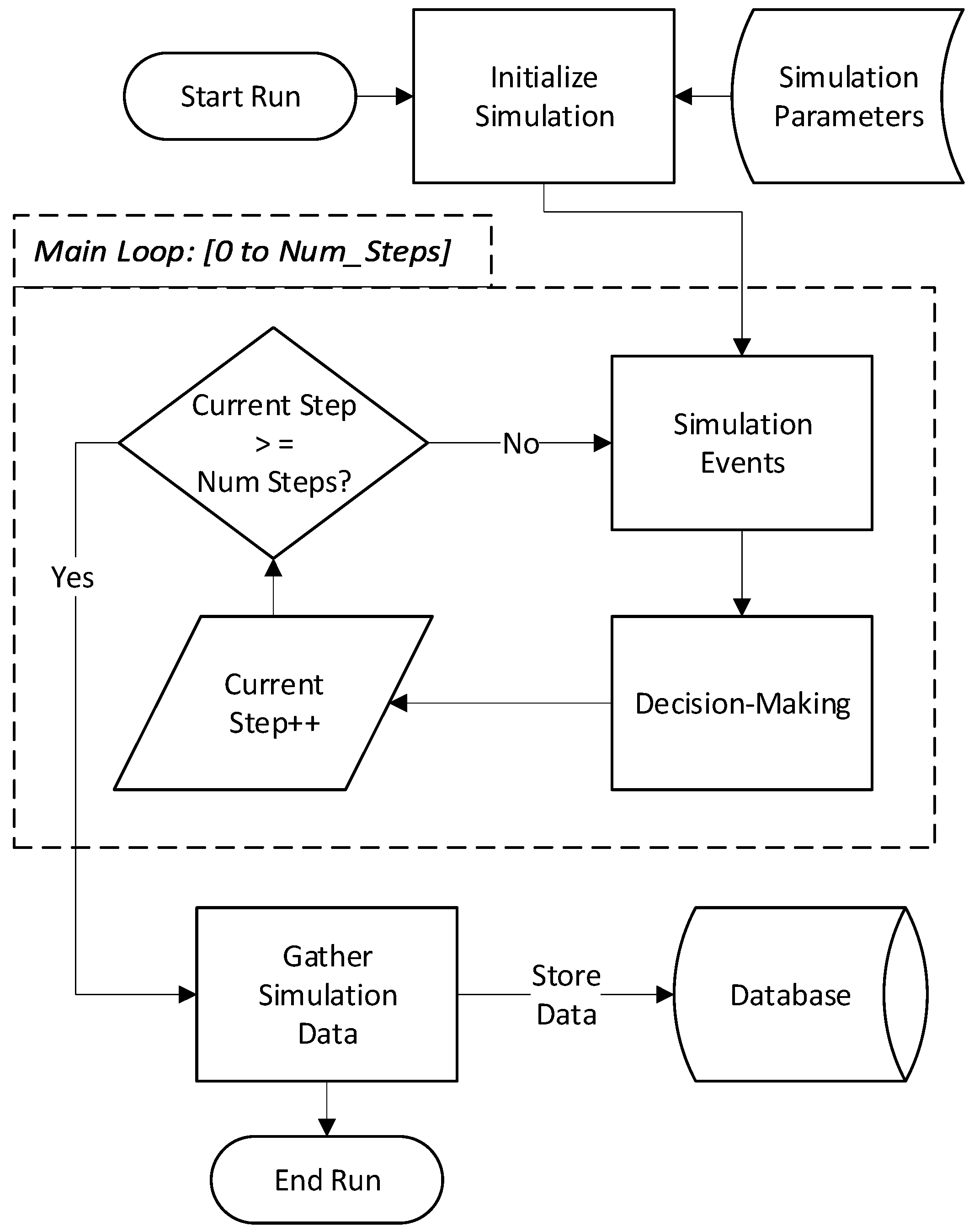
In this section, the operations of the simulation system are detailed. The simulation is divided into a number of iterations (time-steps). The number of time-steps that the system is run for is determined by a user inputted parameter. Each time-step corresponds to a block of time, with the simulation starting at step zero and progressing until the input number of time-steps is reached. A time-step corresponds to an iteration of the main loop, as shown in Figure 7. In the main loop, simulation events occur. This is followed by decision-making (planning) by the robot system. These are discussed in the following subsections.
4.6.1. Simulation Events
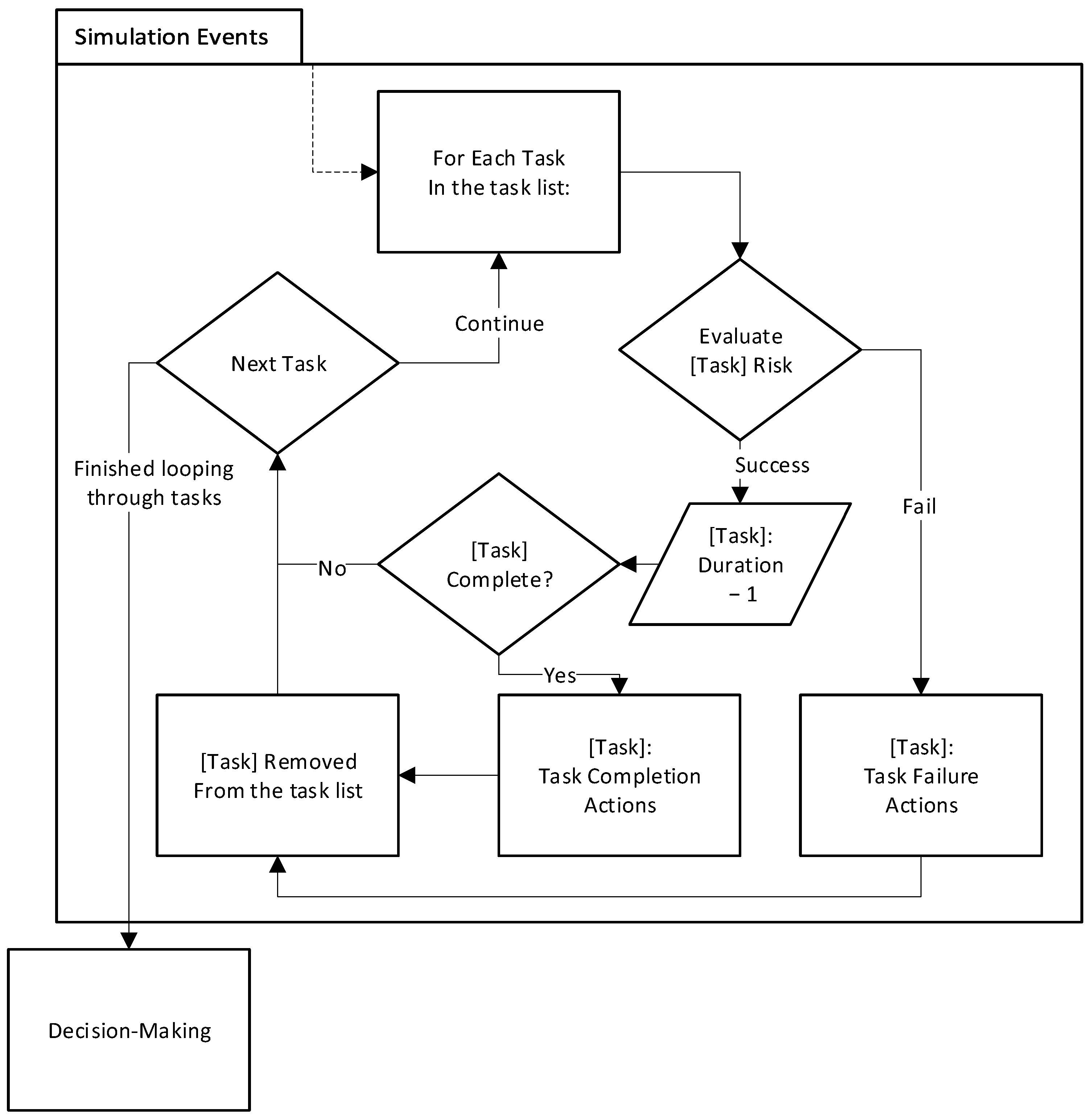
The simulation events step informs the simulated robots’ command systems of the results of the actions of the robot system. During the decision-making step, the SRRS determines what actions to perform in future steps. In each time-step of the simulation, robots in the robot system perform tasks which involve acquiring resources, converting resources, or assembling new robots. The simulation events process determines the results of these actions by the robot system.
The process for processing simulation events, which is depicted in Figure 8, consists of looping through the tasks currently being performed. The tasks currently being performed are determined by the decision-making algorithm and include the tasks for the entire robot system at each time-step of the simulation (i.e., the task list is not a task queue for a single robot but a list of the tasks each robot is currently performing). For each of the tasks in progress by the robot system, the risk of performing the task is used to determine (with random input) if it failed or succeeded in the current time-step. If it succeeded, the task’s remaining duration is decremented by one. If its remaining duration is now zero, then its completion actions are performed (i.e., the resources are gathered, the part is fabricated, or the robot is assembled). In the case where it failed, then the task failure actions are performed, and it is removed from the active tasks, as a failed task is abandoned.
4.6.2. Robot System Decision-Making
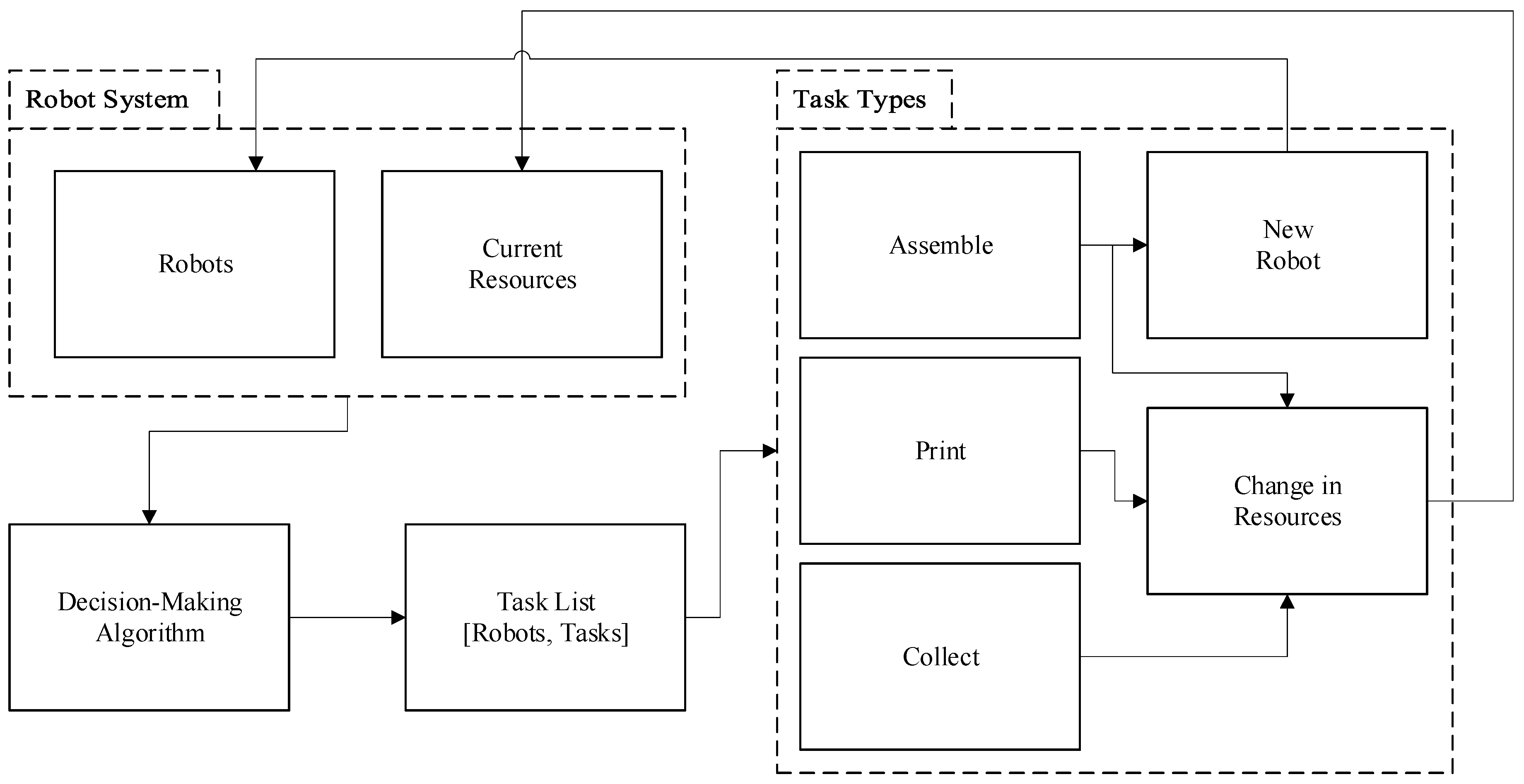
The decision-making process is when the SRRS assigns tasks to the robots (see Figure 9). This includes determining and assigning what robots to build (if any) and which robots should build them, how many robots should print components (if any), and how many robots should collect resources (if any). For the purposes of this work, a simplified decision-making algorithm was utilized to facilitate the analysis of the performance of the different system configurations under the various experimental conditions. This decision-making algorithm is now discussed.
In this algorithm, the choice of when to build a new robot, and what type it should be, is decided with simple criteria. The process begins by identifying all idle assembly-capable robots and then taking the buildable robot type list (see Table 4) and repeating it (in order) until there are enough robots in the build queue for each idle assembly-capable robot. Resource constraints are not checked, initially. If a robot cannot be built, the would-be assembler simply remains idle.
After determining what each of the robots needs to assemble (if anything), the decision-making algorithm assigns all currently idle print-capable robots to fabricate printable components. These assignments are limited by the robot system’s current amount of available raw printing materials (robots will not be assigned to printing tasks that materials are not available for).
After these assignments, all robots that are idle are assigned to collect materials from the environment. If robots return no materials, then it is assumed that the environment is out of raw materials and the system stops assigning any robots to the collection task once this happens. This is, of course, a simplification. The stage at which it can be assumed that no further resources are available to collect may be more complex in real world instances.
5. Experimental Methodology
The goal of the experimentation presented herein is to generate knowledge that can be used to develop decision-making criteria for SRRS decision-making algorithms. The consideration of multiple factors may allow a decision-making system to make more optimal choices, based on the extended set of criteria considered. Thus, in addition to informing decision-making regarding the development of SRRS algorithms, the data presented herein will facilitate the evaluation of future SRRS decision-making algorithms.
In this section, the metrics, experimental conditions, and hypotheses of this study are presented. The primary metrics for which data are collected by the simulation include:
- Assembly capacity: The number of robots that have the assembly capability at the end of a simulation run. This includes replicator and assembler robot types, which have not succumbed to a task risk and lost their capability. The standard deviation of this value, among the simulation runs, is also recorded.
- Collection capacity: The number of robots that have the collect capability at the end of a simulation run. All robot types have this capability in this simulation, so this is always equal to the current number of robots in the system. The standard deviation of this value, among the simulation runs, is also recorded.
- Print capacity: The number of robots that have the print capability at the end of a simulation run. This includes replicator and printer robot types, which have not succumbed to a task risk and lost their capability. The standard deviation of this value, among the simulation runs, is also recorded
5.1. Experimental Conditions
Simulation parameters define each simulation run. These values differ between the experimental conditions in order to facilitate analysis of their impact on the outcome of each simulation run. The simulation parameters and their default values (when not being altered as part of a particular experimental condition) are listed in Table 5.
A list and description of the experimental conditions are presented in Table 6. The values in Table 6 are relative to the default parameter values, and experimental conditions that change multiple parameters, such as experimental condition A16, refer to both parameters changing to the specified value. Each system configuration was run under each experimental condition one hundred times (to infer stochastic elements), with each of three different time-step inputs (“Num_Steps” parameter). These time-step input values were 30, 50, and 70.
5.2. Experiment Hypotheses
There are three hypotheses that the experiments presented in this paper are based on. There is a hypothesis specific to the centralized replication approach. There is one specific to the decentralized and hierarchical replication approaches. There is also one specific to the homogeneous and heterogeneous production approaches. Each is discussed in this section.
5.2.1. Hypothesis 1: Centralized Approach
The hypothesis for the centralized replication approach is that robot build quality will be higher than the decentralized and hierarchical replication approaches. The disadvantage of the centralized approach is that the assembly and printing capabilities are limited to the initial robots, and therefore its assembly and print capacity will be lower than the other replication approaches. Thus, the system collection capacity and average build quality are the metrics of interest. The average build quality is expected to be higher for the centralized replication approach compared to the non-centralized replication approaches for all experimental conditions.
Systems using the centralized replication approach are not expected to have higher collection capacity for the default case, since one assembling robot can only do so much in a given time period. In this regard, the experimental condition classification “C” cases may have instances where the collection capacity begins to favor the centralized replication approach in conditions with increased task risks and build quality demands. Specifically, the higher penalty experimental conditions C4, C7, C8, C9, C12, C13, and C19 are expected to show systems using the centralized approach being more competitive in terms of collection capacity. Secondly, the costs associated with the assemble and print capability do not affect the centralized approach (as only non-replicating robots are built). Thus, a significant enough increase in these parameters may make the centralized approach more competitive in terms of collection capacity. The experimental conditions A6, A9, and A16 are examples where these parameters are significantly increased and are predicted to potentially have this occur.
Experimental condition C18 shows how the benefit of the centralized approach affects the outcome. This benefit is that only the initial robots are assembly capable. The initial robots are assumed to be well tested and therefore have a lower task risk level (simulated using RiskFactory_Modifier). Thus, condition C18 shows the results of the system when that modifier is set to 1.0 (i.e., no task risk reduction for initial robots). It is expected that the collection capacity would be lower due to the robots with an assembly capability succumbing to a task risk more often (on average), and therefore not being able to produce any more robots. The experimental condition C17 is expected to show a similar effect, but to a lesser extent (as it sets the modifier to 0.5).
5.2.2. Hypothesis 2: Decentralized vs. Hierarchical Approach
The hypothesis comparing the decentralized approach to the hierarchical approach is that the assembly and print capacity will be higher in the decentralized approach, as compared to the hierarchical approach. However, the collection capacity for the decentralized approach is expected to be lower than that for the hierarchical approach, as systems using the decentralized approach do not build normal robots (i.e., lower production cost robots that can only collect). Furthermore, the production approach of the system (whether its homogeneous or heterogeneous), may impact performance in this area as well. Thus, it will be of interest to compare the systems using the decentralized replication approach to their hierarchical approach counterpart (and vice versa). Thus, the DHE configuration would be compared to the HHE configuration and the DHO configuration would be compared to the HHO configuration.
The collection capacity is expected to be more equivalent between the decentralized and hierarchical replication approaches when the base production cost values of the robots are increased (and be farther apart when the base production costs are lowered). This is due to the production cost of the normal robots being proportionally raised, which would therefore create a higher cost of building any robot. Experimental conditions A1, A2, and A3 alter the printable components’ costs, A10 increases the required build duration, and A17 increases the nonprintable component costs for all robot types. Given this, it is predicted that under experimental conditions A1, A2, A3, A10, and A17, systems using the decentralized replication approach will have a more equivalent collection capacity (as compared to the default case) to systems using the hierarchical replication approach. However, the nonprintable component cost increase in experimental condition A17 would only affect the system in the later stages (if it affects it) due to potentially causing the system to run out of this resource type.
Systems using the hierarchical replication approach are expected to have a closer print and assembly capacity to systems using the decentralized replication approach in instances where resource collection is more costly. Without enough resources, systems using the decentralized replication approach may not be able to produce robots as quickly. Due to this, it is predicted that under experimental conditions B4 and B5, systems using the hierarchical replication approach will be more competitive, in terms of assembly and print capacity (as compared to systems using the decentralized approach). Experimental conditions B4 and B5 reduce the Collect_Amount parameter, which results in each robot collecting less materials per time-step.
5.2.3. Hypothesis 3: Homogeneous vs. Heterogeneous Approach
The hypothesis comparing the homogeneous and heterogeneous approaches is that the heterogeneous approach will be able to increase the number of robots more rapidly. This prediction is based on the heterogeneous production approach using specialized robots and having a lower production cost, as compared to the homogeneous approach (an exception to this is the CHE configuration, due to its reliance on initial robots). However, over time, the heterogeneous production approach will run out of nonprintable components. Therefore, it is predicted that systems using the homogeneous production approach will have a comparatively greater assembly capacity and print capacity at later stages. This is due to the homogeneous approach using the replicator robot type, which has both print and assemble capabilities. Therefore, fundamentally this experiment is a comparison of the value of versatility versus the value of build speed.
Another mission planning consideration is the relative production costs of the various robot types (both the resources and build time required). Having an asymmetrical cost for the print capability and assemble capability is considered. Due to this, it is predicted that experimental conditions A4, A5, A6, A7, A8 and A9 will result in the DHE and HHE configurations outperforming the DHO and HHO configurations, in terms of collect, print, and assembly capacity.
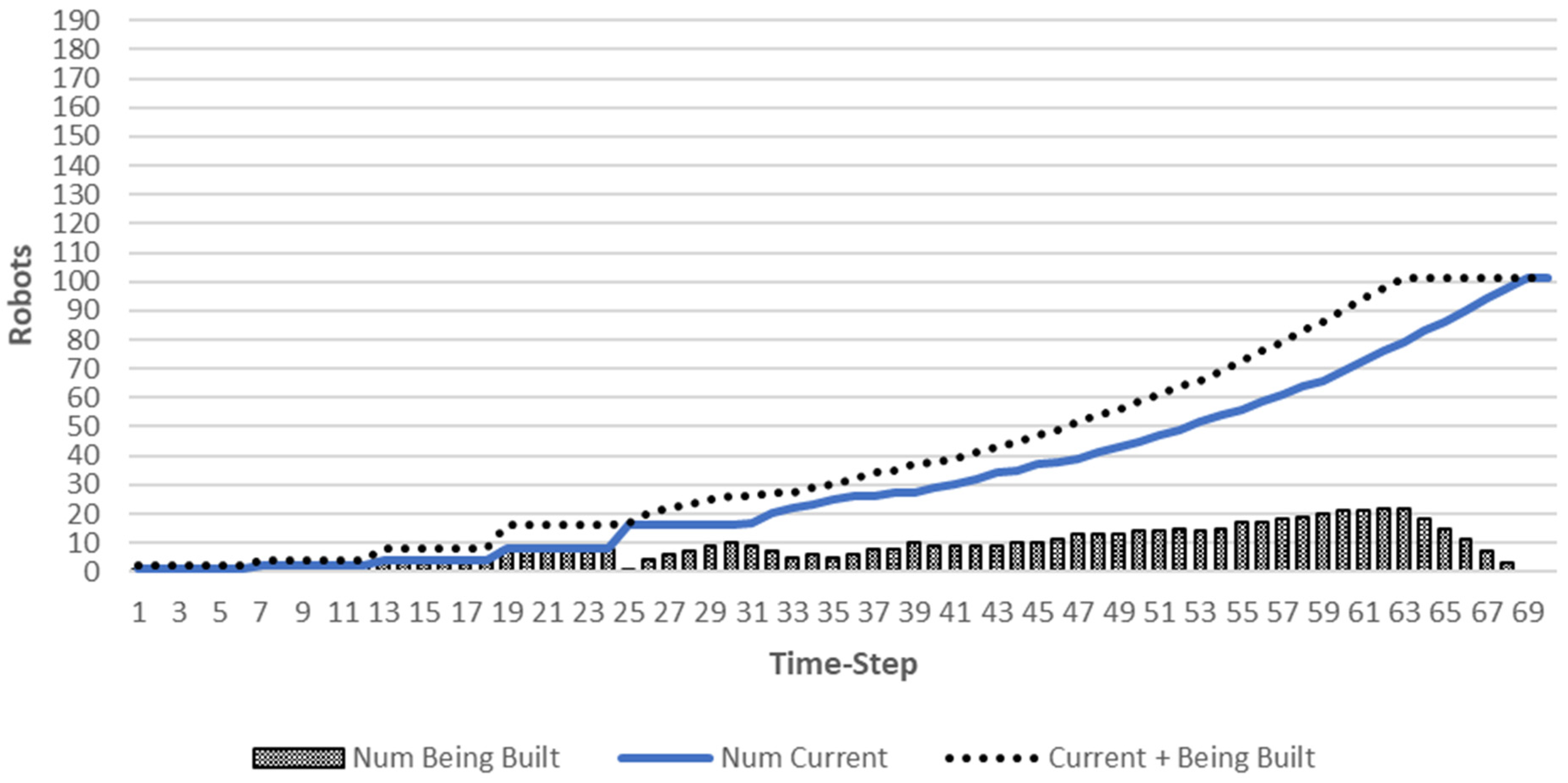
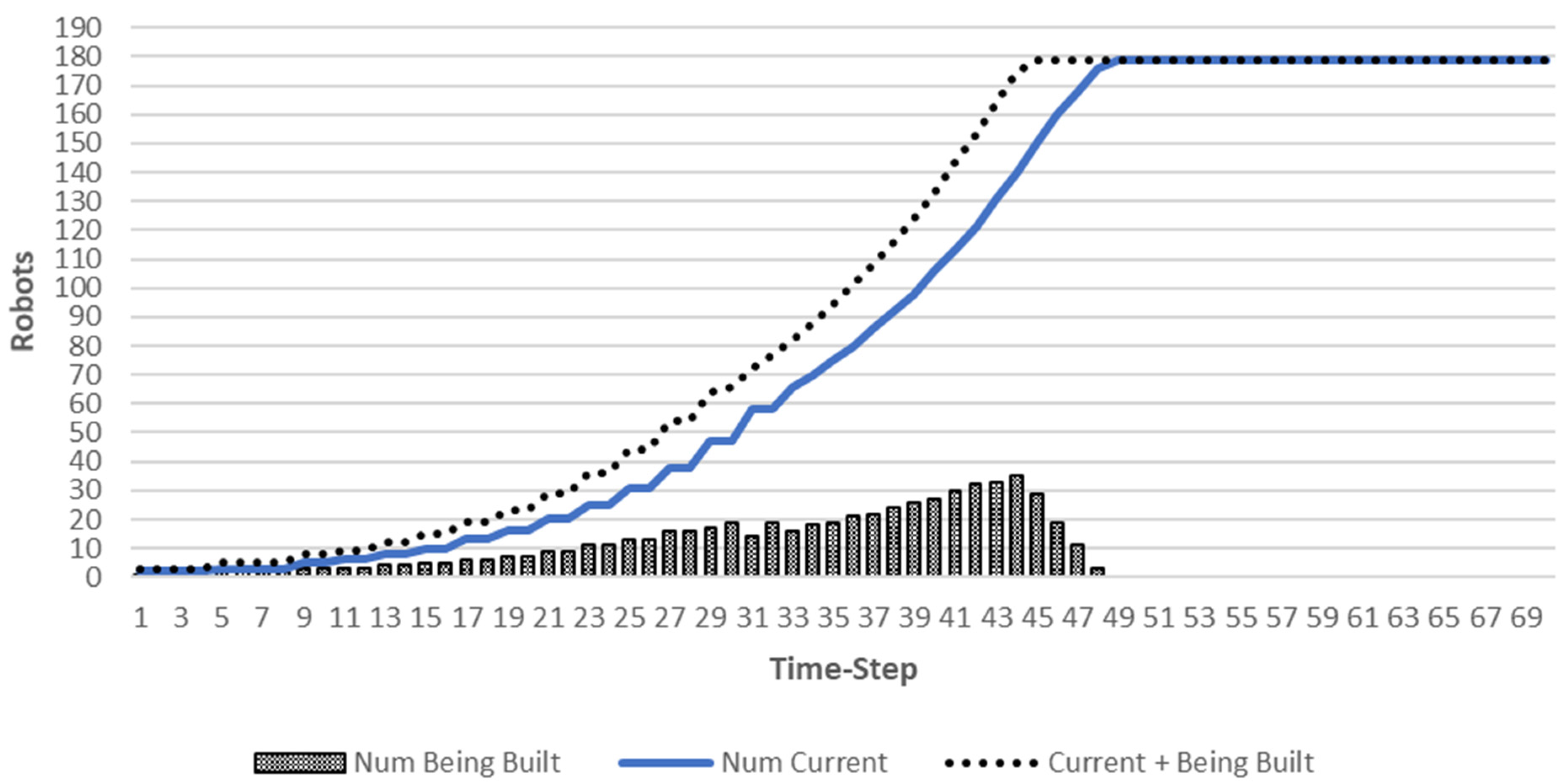
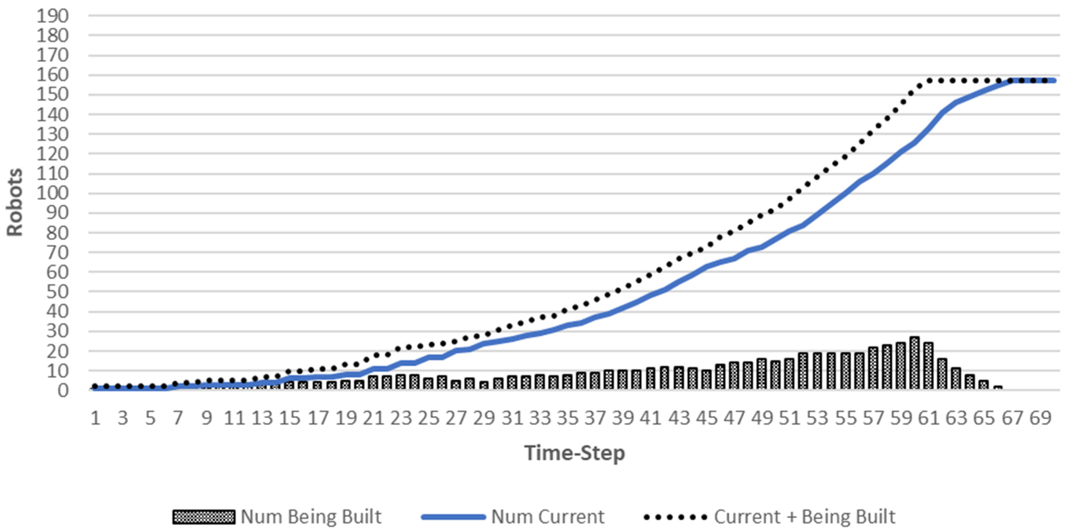
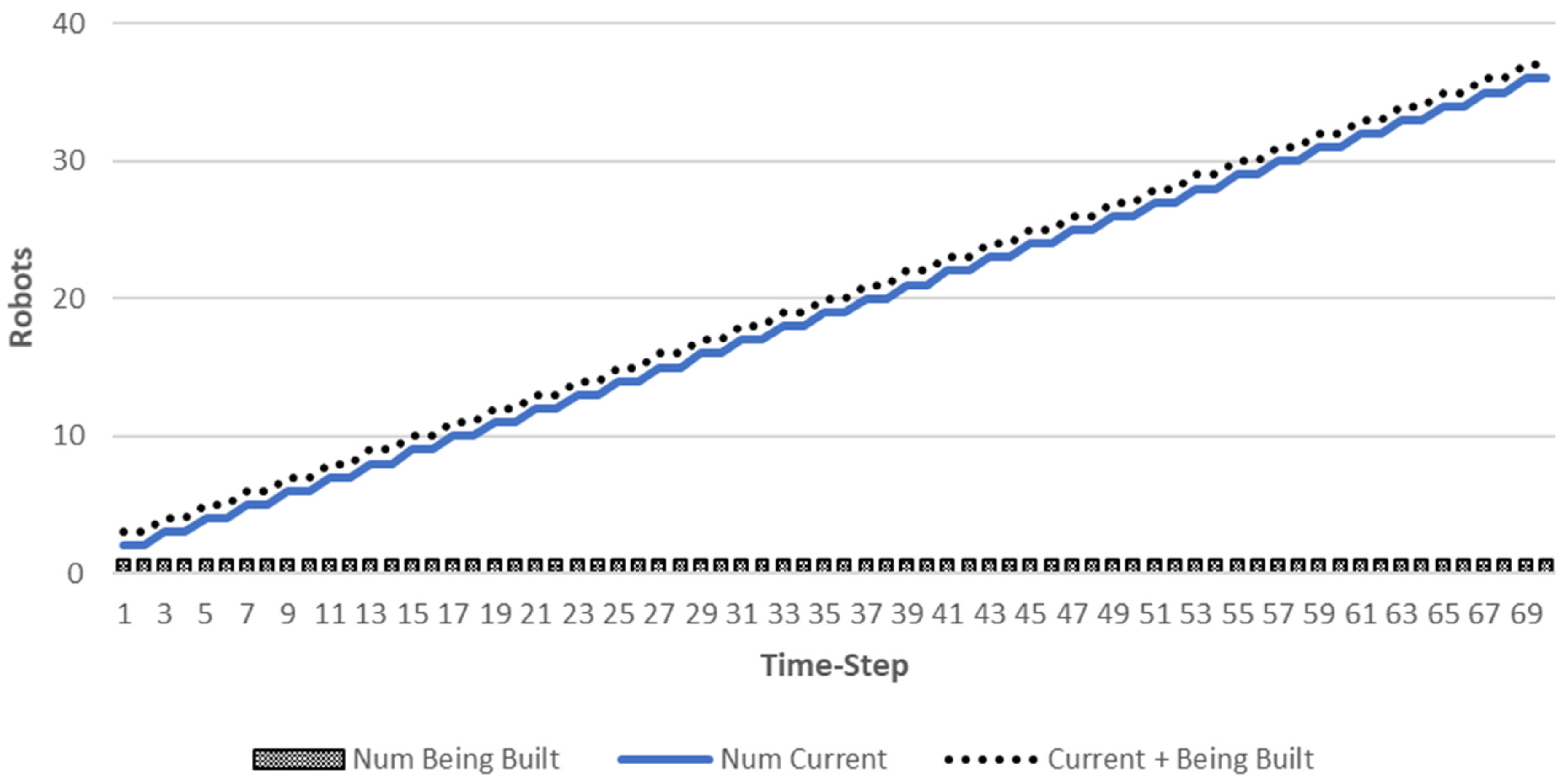
6. Robot Build Rate
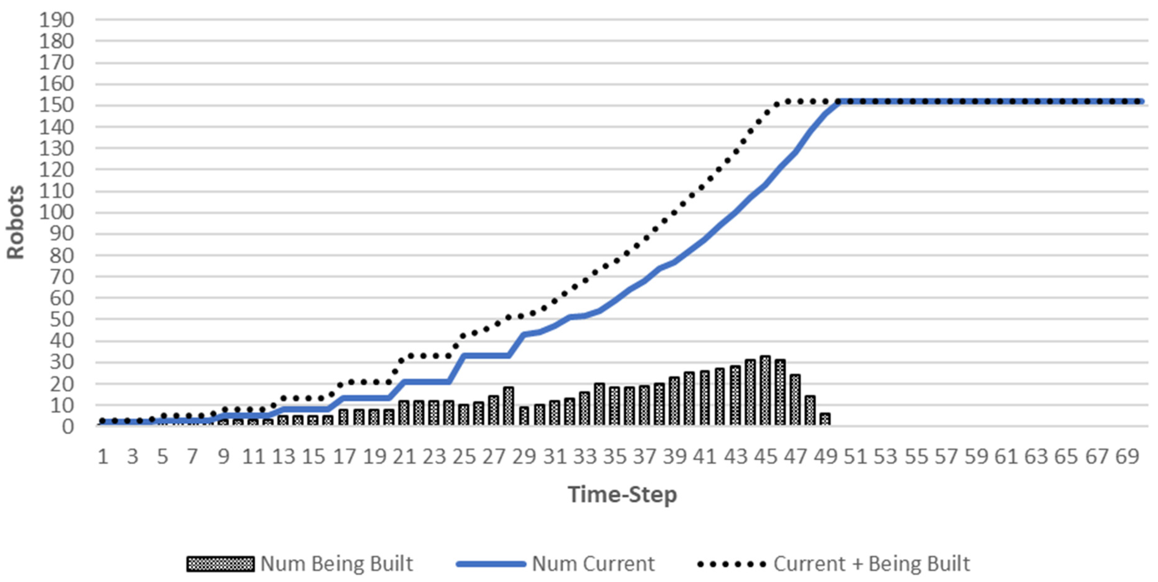
In this section, the robot build rate for each system configuration under experimental condition A0 (the default case) is presented. Figure 10 depicts the build rate for the DHE configuration. Figure 11 depicts the build rate for the DHO configuration. Figure 12 depicts the build rate for the HHE configuration, and Figure 13 depicts the build rate for the HHO configuration. Figure 14 depicts the build rate for the CHE and CHO configurations.
7. Data Analysis
In this section, the data collected during the experimental runs are presented. The results are analyzed to evaluate the hypotheses presented in the previous section. The results are based on one hundred runs of each experimental condition using each system configuration. In the tables, the numbers are the average of these one hundred simulation runs.
7.1. Evaluation of Hypothesis 1: Centralized Categories
The average build quality was predicted to be higher for the system configurations using the centralized replication approach (CHE and CHO) as compared to the other replication approaches. Analysis supports the hypothesis of the average robot build quality being higher for systems using the centralized approach. An average of all experimental conditions for each system configuration for the metric of the average robot build quality is presented in Table 7.
In terms of collection capacity, experimental conditions A6 and A9 did not lower the production of robots for most of the non-centralized configurations enough to make the collection capacity of these systems more comparable to the centralized configurations CHE and CHO. An exception is the DHO configuration, which was lowered enough to be roughly equivalent to the CHE and CHO configurations in terms of collection capacity at time-step 30 (Table 8) and 50 (Table 9). Furthermore, the collection capacity of the CHE and CHO configurations was close to standard deviation range of the DHO configuration at time-step 70 (Table 10).
For experimental conditions C4 and C19, the homogeneous configurations DHO and HHO performed similar to the centralized configurations in terms of collection capacity at the early stages (time-step 30). In the later stages, the HHO configuration was notably higher than the centralized configurations under experimental conditions C4 and C19, while the DHO configuration’s performance remained comparable. In contrast, experimental condition C12 did not result in a significantly different collection capacity, as compared to the default case, and C13 did not lower the collection capacity of the other configurations enough to be similar in value to the CHE and CHO configurations.
The higher risk experimental conditions (C7, C8, and C9) lowered the collection capacity of the non-centralized configurations enough such that the CHE and CHO configurations were competitive. This appears to be primarily attributable to the non-factory built assemble-capable robots having too high a task risk level to assemble, to a functional level, properly in these cases. In comparison, the experimental condition C4 corresponds to having a high rate of build failure (the robot construction failed). Under experimental conditions C7, C8, and C9, the dynamic is slightly different in that the risk involves the assembling robot failing during the assembly process and thus losing the assemble capability. In this case, not only does the build fail, but the assembling robot also loses its capability. The results support the hypothesis that the non-centralized configurations are, to some extent, able to better cope with a high rate of build failure but are less able to cope with a high rate of assembly equipment failure.
Finally, experimental conditions C17 and C18 did not show a significant impairment of collection capacity, as compared to the default case. With a 0.1% chance of the assembly robot losing the assemble capability per time-step (due to the task risk level), failure did not occur enough to have a significant impact.
7.2. Evaluation of Hypothesis 2: Decentralized versus Hierarchical
The results from the default experimental condition (A0) support the hypothesis that the hierarchical categories have a higher collection capacity, as compared to their decentralized counterparts (depicted in Figure 5, Figure 6, Figure 7 and Figure 8). Furthermore, the decentralized categories have demonstrated an increased print and assembly capacity, as compared to their hierarchical counterparts (as shown in Table 11). Both of these facts support this hypothesis as well.
Experimental conditions A1, A2, and A3 affect the Base_CostPr parameter on an increasing scale. For these three experimental conditions, the decentralized configurations were closer, in terms of collection capacity, to the hierarchical configurations than the default case. Unexpectedly, the DHE configuration outperformed the HHE configuration under experimental condition A2 at the time-steps of 50 and 70. In addition, it outperformed for experimental condition A3 by a marginal amount at time-step 50 (and was approximately equivalent to the highest performing conditions at time-steps 30 and 70). This supports the hypothesis that raising the base production cost of robots (in terms of printable components) increases the comparative performance of decentralized configurations, compared to hierarchical configurations, in terms of collection capacity. Although, it is more prevalent for the DHE configuration, as compared to the HHE configuration, and more marginal of a comparative gain for the DHO configuration versus the HHO configuration.
Experimental condition A10 involves increasing the BaseCost_Time parameter, which affects how long it takes to build all robot types. While this was hypothesized to potentially favor the collection capacity of decentralized configurations over hierarchical configurations, the results showed a pattern similar to a slowly progressing default case (A0). Experimental condition A17 increases the nonprintable component cost for all robots (BaseCost_NonPr), and the results indicate that this did not significantly enhance the comparative performance of the decentralized approach, as compared to the hierarchical approach.
Experimental conditions B4 and B5 involve reducing the Collect_Amount parameter, where B4 reduces it by a factor of four and B5 reduces it by half. These two experimental conditions affected the performance of the decentralized configurations, as compared to the hierarchical configurations in terms of assembly capacity and print capacity (shown in Table 11). The HHE configuration was approximately equal to the DHE configuration in terms of print and assembly capacity under experimental conditions B4 and B5 at time-step 50. However, under experimental condition B5, this converged to approximately the same as the default case by time-step 70, presumably due to reaching the maximum number of robots within resource constraints. The HHO configuration approximately equaled the DHO configuration at time-step 50 and notably outperformed it at time-step 70. These results differ from the default case, where the DHO configuration outperformed the HHO configuration, and the DHE configuration outperformed the HHE configuration.
7.3. Evaluation of Hypothesis 3: Heterogeneous versus Homogeneous
The results of the default experimental condition (A0) support the hypothesis that the heterogeneous DHE and HHE configurations produce robots more rapidly than the homogeneous DHO and HHO configurations. Under this experimental condition, the DHE and HHE configurations reached the resource-constraint-based maximum number of robots by time-step 50 (as depicted in Figure 5 and Figure 7). In contrast, the DHO and HHO configurations showed a more linear build rate, which reached the maximum number of robots around time-step 70 (as depicted in Figure 6 and Figure 8). Thus, the DHO and HHO configurations outperformed their heterogeneous counterparts in terms of assembly and print capacity by time-step 70. This supports the hypothesis that the homogeneous production approach would have a greater assembly capacity and print capacity than the heterogeneous production approach at later time-steps.
In terms of assembly capacity, the DHE and HHE configurations continued to outperform their homogeneous counterparts at time-step 70 under experimental conditions A5, A6, A8, and A9 (as shown in Table 12). Similarly, in terms of print capacity, the DHE and HHE configurations outperformed under experimental conditions A5, A8, and A9 (but not for A6) at time-step 70.
The experimental conditions A4 and A7, which increase printable cost to a lesser extent, resulted in the DHE and HHE configurations performing closer (as compared to A0) to their homogeneous counterpart at time-step 70, for both assembly and print capacity. Thus, the increase in the printable component cost appears to comparatively favor the heterogeneous production approach over the homogeneous production approach. This provides support for the hypothesis that the heterogeneous production approach is able to continue to outperform the homogeneous approach, in terms of assembly and print capacity, for these experimental conditions, even when robot numbers reach a resource constrained maximum.
8. Conclusions
This paper considered questions of how to best design and command an SRRS. A simulation system for SRRSs was presented and an experiment was conducted using it. The experiment studied the differences in performance caused by the system configuration decisions. The heterogeneous configurations of DHE and HHE (not configuration CHE) were shown to reach a maximum number of robots (based on available resources) more quickly than their homogeneous configuration counterparts. However, the homogeneous configurations DHO and HHO outperformed them in terms of assembly capacity and print capacity in later time-steps (under many experimental conditions). The decentralized configurations DHE and DHO outperformed their hierarchical counterparts in terms of assembly capacity and print capacity under most experimental conditions; however, they had a lower collection capacity. Whether a system was a homogeneous or heterogeneous configuration was shown to be a significant factor, overall, in its performance.
These findings, along with the data acquired from the experiment in this paper, could potentially be used to establish decision-making criteria for SRRS decision-making algorithms. The data from the various experimental conditions in the experiment could potentially be used as a heuristic to optimize the SRRS based on the ratio of printable component costs to in-situ resource collection rate and the rate at which the in-situ resources are converted into printable components. Planned future work includes the use of these data for analyzing the comparative efficacy of the decision-making algorithms.
Author Contributions
Conceptualization, A.J. and J.S.; data curation, A.J.; methodology, A.J. and J.S.; resources, J.S.; software, A.J.; supervision, J.S.; writing—original draft, A.J.; writing—review & editing, J.S. All authors have read and agreed to the published version of the manuscript.
Funding
Andrew Jones was supported by the North Dakota Space Grant Consortium for a portion of this project.
Informed Consent Statement
Not applicable.
Data Availability Statement
The data presented in this study are available on request from the corresponding author and will be made publicly available at a later time.
Acknowledgments
Facilities, materials, and equipment used for this work have been supplied by the North Dakota State University (NDSU) Department of Computer Science, the NDSU Foundation and the NDSU College of Science and Math.
Conflicts of Interest
The authors declare no conflict of interest.
References
- Sipper, M. Fifty Years of Research on Self-Replication: An Overview. Artif. Life 1998, 4, 237–257. [Google Scholar] [CrossRef]
- Sanders, G.B. Advancing in situ resource utilization capabilities to achieve a new paradign in space exploration. In Proceedings of the 2018 AIAA SPACE and Astronautics Forum and Exposition, Orlando, FL, USA, 17–19 September 2018; American Institute of Aeronautics and Astronautics Inc.: Reston, VA, USA, 2018. [Google Scholar]
- Jones, A.; Straub, J. Concepts for 3D Printing-Based Self-Replicating Robot Command and Coordination Techniques. Machines 2017, 5, 12. [Google Scholar] [CrossRef] [Green Version]
- Jones, A.B.; Straub, J. Mission-Responsive. On-Demand 3D Printed Blimps for Martian Missions. In Proceedings of the IEEE Aerospace Conference, Big Sky, MT, USA, 2–9 March 2019; pp. 1–6. [Google Scholar]
- Von Neumann, J. The Theory of Self Reproducing Automata, 1st ed.; Burks, A.W., Ed.; University of Illinois Press: Champaign, IL, USA, 1966; ISBN 0252727339. [Google Scholar]
- Suthakorn, J.; Kwon, Y.T.; Chirikjian, G.S. A semi-autonomous replicating robotic system. In Proceedings of the Proceedings 2003 IEEE International Symposium on Computational Intelligence in Robotics and Automation, Kobe, Japan, 16–20 July 2003; Volume 2, pp. 776–781. [Google Scholar]
- Beuchat, J.-L.; Haenni, J.O. Von Neumann’s 29-state cellular automaton: A hardware implementation. IEEE Trans. Educ. 2000, 43, 300–308. [Google Scholar] [CrossRef]
- Jones, R.; Haufe, P.; Sells, E.; Iravani, P.; Olliver, V.; Palmer, C.; Bowyer, A. RepRap the replicating rapid prototyper. Robotica 2011, 29, 177–191. [Google Scholar] [CrossRef] [Green Version]
- Jones, A.; Straub, J. Student Benefits from Participation in a NASA-mentored 3D Printing Research Project. In Proceedings of the Midwest Instruction and Computing Symposium, Duluth, MN, USA, 6–7 April 2018. [Google Scholar]
- Chua, C.K.; Leong, K.F. 3D Printing and Additive Manufacturing: Principles and Applications; World Scientific Publishing Company: Singapore, 2015; ISBN 9789814571418. [Google Scholar]
- Campbell, T.; Williams, C.; Ivanova, O.; Garrett, B. Could 3D Printing Change the World? Technologies, Potential, and Implications of Additive Manufacturing, Atlantic Council: Washington, DC, USA, October 2011; pp. 1–14. [Google Scholar]
- Berman, B. 3-D printing: The new industrial revolution. Bus. Horiz. 2012, 55, 155–162. [Google Scholar] [CrossRef]
- Schubert, C.; van Langeveld, M.C.; Donoso, L.A. Innovations in 3D printing: A 3D overview from optics to organs. Br. J. Ophthalmol. 2014, 98, 159–161. [Google Scholar] [CrossRef] [PubMed]
- Pfeifer, T.; Koch, C.; Hulle, L. Van Optimization of the FDMTM Additive Manufacturing Process. In Proceedings of the Annual Technical Conference (ANTEC) of the Society of Plastics Engineers, Indianapolis, IN, USA, 23–25 May 2016. [Google Scholar]
- Stroud, A.B.; Morris, M.; Carey, K.; Williams, J.C.; Randolph, C.; Williams, A.B. MU-L8: The Design Architecture and 3D Printing of a Teen-Sized Humanoid Soccer Robot. In Proceedings of the Workshop on Humanoid Soccer Robots, Atlanta, GA, USA, 15 October 2013. [Google Scholar]
- Kading, B.; Straub, J. Utilizing in-situ resources and 3D printing structures for a manned Mars mission. Acta Astronaut. 2015, 107, 317–326. [Google Scholar] [CrossRef]
- Cesaretti, G.; Dini, E.; De Kestelier, X.; Colla, V.; Pambaguian, L. Building components for an outpost on the Lunar soil by means of a novel 3D printing technology. Acta Astronaut. 2014, 93, 430–450. [Google Scholar] [CrossRef]
- Chirikjian, G.S.; Zhou, Y.; Suthakorn, J. Self-replicating robots for lunar development. IEEE/ASME Trans. Mechatron. 2002, 7, 462–472. [Google Scholar] [CrossRef]
- Winfield, A.F. Foraging Robots. In Encyclopedia of Complexity and Systems Science; Springer: New York, NY, USA, 2009; Volume 6, pp. 3682–3700. ISBN 9780387758886. [Google Scholar]
- Waters, K.H. Reflection Seismology: A Tool for Energy Resource Exploration, 3rd ed.; Wiley-Interscience: Hoboken, NJ, USA, 1987. [Google Scholar]
- LeCun, Y.; Bengio, Y.; Hinton, G. Deep learning. Nature 2015, 521, 436–444. [Google Scholar] [CrossRef] [PubMed]
- Green, J.J.; Vogt, D. A Robot Miner for Low Grade Narrow Tabular Ore Bodies: The Potential and the Challenge. In Proceedings of the 3rd Robotics and Mechatronics Symposium, Pretoria, South Africa, 8–10 November 2009. [Google Scholar]
- Shaffer, G.; Stentz, A. A robotic system for underground coal mining. In Proceedings of the IEEE International Conference on Robotics and Automation, Nice, France, 12–14 May 1992; Volume 1, pp. 633–638. [Google Scholar]
- Dunker, P.A.; Lewinger, W.A.; Hunt, A.J.; Quinn, R.D. A Biologically Inspired Robot for Lunar Exploration and Regolith Excavation. In Proceedings of the IEEE International Conference on Intelligent Robots and Systems, Shanghai, China, 20–22 November 2009; pp. 5039–5044. [Google Scholar]
- Freitas, R.A.; Merkle, R.C. Kinematic Self-Replicating Machines; Landes Bioscience: Georgetown, TX, USA, 2004; ISBN 9781570596902. [Google Scholar]
- Yan, Z.; Jouandeau, N.; Cherif, A.A. A Survey and Analysis of Multi-Robot Coordination. Int. J. Adv. Robot. Syst. 2013, 10, 399. [Google Scholar] [CrossRef]
- Jones, A.; Straub, J. Self-replicating 3d printed satellites. In Proceedings of the International Astronautical Congress, Adelaide, Australia, 25–29 September 2017; Volume 13, pp. 8264–8271. [Google Scholar]
- Snappy. Available online: http://reprap.org/wiki/Snappy (accessed on 18 July 2017).
- Timmiclark MR 4: Robotic Tank. Available online: https://www.thingiverse.com/thing:1906831 (accessed on 4 March 2020).
- Gerkey, B.P. On Multi-Robot Task Allocation; University of Southern California: Los Angeles, CA, USA, 2003. [Google Scholar]
- Welch, R.; Limonadi, D.; Manning, R. Systems engineering the Curiosity rover: A retrospective. In Proceedings of the 2013 8th International Conference on System of Systems Engineering: SoSE in Cloud Computing and Emerging Information Technology Applications, Maui, HI, USA, 2–6 June 2013; pp. 70–75. [Google Scholar]
- Khoshnevis, B.; Carlson, A.; Thangavelu, M. ISRU-Based Robotic Construction Technologies for Lunar and Martian Infrastructures; University of Southern California: Los Angeles, CA, USA, 2013. [Google Scholar]
- Nygaard, T.F.; Martin, C.P.; Samuelsen, E.; Torresen, J.; Glette, K. Real-world evolution adapts robot morphology and control to hardware limitations. In Proceedings of the 2018 Genetic and Evolutionary Computation Conference, Kyoto, Japan, 15–19 July 2018; pp. 125–132. [Google Scholar]
- Salvador, R.; Otero, A.; Mora, J.; de la Torre, E.; Sekanina, L.; Riesgo, T. Fault tolerance analysis and self-healing strategy of autonomous, evolvable hardware systems. In Proceedings of the 2011 International Conference on Reconfigurable Computing and FPGAs, Cancun, Mexico, 30 November–2 December 2011; pp. 164–169. [Google Scholar]
Figure 1.
Conceptual diagram of the centralized replication approach.

Figure 2.
Conceptual diagram of the decentralized replication approach.

Figure 3.
Conceptual diagram of the hierarchical replication approach.

Figure 4.
Conceptual Prototype of a 3D-printed 3D print-capable robot. The left image shows an in-progress 3D print.
Figure 4.
Conceptual Prototype of a 3D-printed 3D print-capable robot. The left image shows an in-progress 3D print.

Figure 5.
Conceptual prototype of a 3D-printed resource locating robot.

Figure 6.
Diagram depicting how task types are related to resource types.

Figure 7.
Diagram of the high-level operations of the simulation.

Figure 8.
Diagram depicting the operation of simulation events.

Figure 9.
Diagram depicting an overview of the decision-making system responsibilities.

Figure 10.
Robot build rate of the decentralized heterogeneous (DHE) configuration on experimental condition A0.
Figure 10.
Robot build rate of the decentralized heterogeneous (DHE) configuration on experimental condition A0.

Figure 11.
Robot build rate of the decentralized homogeneous (DHO) configuration on experimental condition A0.
Figure 11.
Robot build rate of the decentralized homogeneous (DHO) configuration on experimental condition A0.

Figure 12.
Robot build rate of the hierarchical heterogeneous (HHE) configuration on experimental condition A0.
Figure 12.
Robot build rate of the hierarchical heterogeneous (HHE) configuration on experimental condition A0.

Figure 13.
Robot build rate of the hierarchical homogeneous (HHO) configuration on experimental condition A0.
Figure 13.
Robot build rate of the hierarchical homogeneous (HHO) configuration on experimental condition A0.

Figure 14.
Robot build rate of the centralized heterogeneous (CHE) and decentralized heterogeneous (CHO) configurations on experimental condition A0.
Figure 14.
Robot build rate of the centralized heterogeneous (CHE) and decentralized heterogeneous (CHO) configurations on experimental condition A0.


Table 1.
Initial resources.
| Initial Nonprintable | Initial Printable | Initial Materials | Environment Materials |
|---|---|---|---|
| 300.0 | 100.0 | 50.0 | 500.0 |
Table 2.
Robot capabilities based on type of robot.
| Robot Type | Collect Resources | Print Components | Assemble Robots |
|---|---|---|---|
| Normal | ● | ||
| Assembler | ● | ● | |
| Printer | ● | ● | |
| Replicator | ● | ● | ● |
Table 3.
Default resource costs by capability.
| Cost per Capability | Nonprintable Cost (NonPr) | Printable Cost (Pr) | Build Duration Cost (Time) |
|---|---|---|---|
| Base (BaseCost) | 1 | 2 | 2 |
| Printing Capability (PrintCost) | 1 | 2 | 2 |
| Assemble Capability (AssembleCost) | 1 | 2 | 2 |
Table 4.
Buildable robot types by robot system configuration.
| Buildable Robot Types | Centralized | Decentralized | Hierarchical |
|---|---|---|---|
| Homogeneous | Normal | Replicator | Replicator, Normal |
| Heterogeneous | Normal | Assembler, Printer | Assembler, Printer, Normal |
Table 5.
List of simulation parameters.
| Parameter | Default Value | Description |
|---|---|---|
| Num_Steps | - | Number of iterations/time-steps that the simulation goes through. |
| Initial_NonPr | 300.0 | The robot system’s starting quantity of nonprintable components. |
| Initial_Printable | 100.0 | The robot system’s starting quantity of printable components. |
| Initial_Materials | 50.0 | The robot system’s starting quantity of raw printing materials. |
| Env_Materials | 500.0 | The environment’s quantity of collectable raw printing materials. |
| BaseCost_NonPr | 1 | Base robot cost of nonprintable components. |
| PrintCost_NonPr | 1 | Print capability cost of nonprintable components. |
| AssembleCost_NonPr | 1 | Assemble capability cost of nonprintable components. |
| BaseCost_Pr | 2 | Base robot cost of printable components. |
| PrintCost_Pr | 2 | Print capability cost of printable components. |
| AssembleCost_Pr | 2 | Assemble capability cost of printable components. |
| BaseCost_Time | 2 | Base robot cost of build time (in time-steps). |
| PrintCost_Time | 2 | Print capability cost of build time (in time-steps). |
| AssembleCost_Time | 2 | Assemble capability cost of build time (in time-steps). |
| Print_Efficiency | 1.0 | Factor that scales raw printing materials to printable components. |
| Print_Amount | 1.0 | Amount of raw materials converted per print task. |
| Collect_Amount | 1.0 | Raw printing materials per collecting robot per timestep. |
| QualityThreshold | 0.5 | Robots with a quality below this are non-functional. |
| Quality_incr_Chance | 5.0% | Chance that a new robot’s build quality will increase. |
| Quality_incr_Lower | 0.01 | Lower bound for quality increase amount. |
| Quality_incr_Upper | 0.05 | Upper bound for quality increase amount. |
| Quality_decr_Chance | 50.0% | Chance that a new robot’s build quality will decrease. |
| Quality_decr_Lower | 0.01 | Lower bound for quality decrease amount. |
| Quality_decr_Upper | 0.25 | Upper bound for quality decrease amount. |
| RiskAmount_Collect | 1.0% | Risk chance for the collect task type. |
| RiskAmount_Assemble | 0.1% | Risk chance for the assemble task type. |
| RiskAmount_Print | 0.1% | Risk chance for the print task type. |
| RiskQuality_Modifier | 5.0 | Multiplier for impact of quality defects on risk amount. |
| RiskFactory_Modifier | 0.1 | Multiplier for impact of factory-made robots on risk amount. |
Table 6.
List of experimental conditions.
| ID | Experimental Condition | Description |
|---|---|---|
| A0 | (Default) | Default values for all parameters. |
| A1 | BaseCost_Pr + 1 | BaseCost_Pr increased from 2 to 3. |
| A2 | BaseCost_Pr + 3 | BaseCost_Pr increased from 2 to 5. |
| A3 | BaseCost_Pr + 5 | BaseCost_Pr increased from 2 to 7. |
| A4 | PrintCost_Pr + 1 | PrintCost_Pr increased from 2 to 3. |
| A5 | PrintCost_Pr + 3 | PrintCost_Pr increased from 2 to 5. |
| A6 | PrintCost_Pr + 5 | PrintCost_Pr increased from 2 to 7. |
| A7 | AssembleCost_Pr + 1 | AssembleCost_Pr increased from 2 to 3. |
| A8 | AssembleCost_Pr + 3 | AssembleCost_Pr increased from 2 to 5. |
| A9 | AssembleCost_Pr + 5 | AssembleCost_Pr increased from 2 to 7. |
| A10 | BaseCost_Time + 2 | BaseCost_Time increased from 2 to 4. |
| A16 | Print & Assemble Time + 2 | PrintCost_Time and AssembleCost_Time increased to 4. |
| A17 | BaseCost_NonPr + 1 | BaseCost_NonPr increased from 1 to 2. |
| B4 | Collect_Amount = 0.25 | Collect_Amount decreased from 1.0 to 0.25. |
| B5 | Collect_Amount = 0.5 | Collect_Amount decreased from 1.0 to 0.5. |
| C4 | QualityThreshold + 0.4 | QualityThreshold increased from 0.5 to 0.9. |
| C7 | RiskAmount Pr & As = 10% | RiskAmount_Print & RiskAmount_Assemble = 10%. |
| C8 | RiskAmount Pr & As = 15% | RiskAmount_Print & RiskAmount_Assemble = 15%. |
| C9 | RiskAmount_Assemble = 15% | RiskAmount_Assemble increased from 0.1% to 15%. |
| C10 | Quality_incr_Chance = 0.01% | Quality_incr_Chance decreased from 5% to 0.01%. |
| C11 | Quality_decr_Chance = 25% | Quality_decr_Chance decreased from 50% to 25%. |
| C12 | Quality_decr_Chance = 75% | Quality_decr_Chance increased from 50% to 75%. |
| C13 | Quality_decr_Upper = 0.5 | Quality_decr_Upper increased from 0.25 to 0.5. |
| C17 | RiskFactory_Modifier = 0.5 | RiskFactory_Modifier increased from 0.1 to 0.5. |
| C18 | RiskFactory_Modifier = 1.0 | RiskFactory_Modifier increased from 0.1 to 1.0. |
| C19 | Quality Thres & decr_Chance | QualityThreshold = 0.9 & Quality_decr_Chance = 75%. |
Table 7.
Average robot build quality across all experimental conditions.
| CHE | CHO | DHE | DHO | HHE | HHO | |
|---|---|---|---|---|---|---|
| TIME-STEP: 30 | 0.945 | 0.942 | 0.875 | 0.887 | 0.876 | 0.875 |
| TIME-STEP: 50 | 0.942 | 0.940 | 0.854 | 0.873 | 0.852 | 0.855 |
| TIME-STEP: 70 | 0.941 | 0.939 | 0.850 | 0.860 | 0.850 | 0.846 |
Table 8.
Centralized hypothesis-related data for time-step 30.
| (30) | Experimental Condition | Collection Capacity | |||||
|---|---|---|---|---|---|---|---|
| CHE | CHO | DHE | DHO | HHE | HHO | ||
| A0 | (Default) | 13.77 | 12.84 | 41.33 | 15.78 | 44.19 | 23.19 |
| A6 | PrintCost_Pr + 5 | 13.42 | 12.67 | 31.96 | 11.77 | 39.31 | 26.25 |
| A9 | AssembleCost_Pr + 5 | 13.93 | 12.83 | 26.57 | 11.75 | 33.99 | 25.83 |
| A16 | Print & Assemble Time + 2 | 13.73 | 12.57 | 12.73 | 3.95 | 17.26 | 6.61 |
| C4 | QualityThreshold + 0.4 | 10.72 | 9.30 | 21.23 | 8.20 | 21.75 | 11.12 |
| C7 | RiskAmount Pr & As = 10% | 12.24 | 11.07 | 14.15 | 6.79 | 13.93 | 8.70 |
| C8 | RiskAmount Pr & As = 15% | 11.32 | 10.45 | 10.92 | 5.00 | 10.71 | 7.03 |
| C9 | RiskAmount_Assemble = 15% | 11.87 | 10.35 | 10.67 | 5.04 | 11.53 | 6.95 |
| C12 | Quality_decr_Chance = 75% | 13.40 | 12.34 | 39.71 | 15.26 | 42.87 | 22.26 |
| C13 | Quality_decr_Upper = 0.5 | 13.15 | 12.57 | 35.69 | 12.96 | 38.06 | 20.12 |
| C17 | RiskFactory_Modifier = 0.5 | 13.81 | 12.72 | 41.68 | 15.73 | 43.42 | 23.16 |
| C18 | RiskFactory_Modifier = 1.0 | 13.41 | 12.26 | 40.87 | 15.54 | 43.41 | 22.88 |
| C19 | Quality Thres & Chance | 8.73 | 7.23 | 12.64 | 5.21 | 12.04 | 7.22 |
Table 9.
Centralized hypothesis-related data for time-step 50.
| (50) | Collection Capacity | Collection Capacity Std Dev | ||||||||||
|---|---|---|---|---|---|---|---|---|---|---|---|---|
| CHE | CHO | DHE | DHO | HHE | HHO | CHE | CHO | DHE | DHO | HHE | HHO | |
| A0 | 20.25 | 18.81 | 129.48 | 39.28 | 164.48 | 66.46 | 2.07 | 1.98 | 11.67 | 3.15 | 7.92 | 3.83 |
| A6 | 19.88 | 19.24 | 71.88 | 19.72 | 97.06 | 63.05 | 2.11 | 2.58 | 5.00 | 2.14 | 5.12 | 4.35 |
| A9 | 19.96 | 18.77 | 57.51 | 19.20 | 80.82 | 62.44 | 2.29 | 2.07 | 5.44 | 2.70 | 7.47 | 4.60 |
| A16 | 19.43 | 18.79 | 54.32 | 15.43 | 70.05 | 27.61 | 2.27 | 2.06 | 3.19 | 0.82 | 5.00 | 2.54 |
| C4 | 15.02 | 14.79 | 53.19 | 20.79 | 64.19 | 30.73 | 2.58 | 2.32 | 12.13 | 4.93 | 16.30 | 9.35 |
| C7 | 16.01 | 14.89 | 22.62 | 11.48 | 23.07 | 15.44 | 6.71 | 6.76 | 9.99 | 5.86 | 10.40 | 8.41 |
| C8 | 14.68 | 12.54 | 13.89 | 7.75 | 15.13 | 10.50 | 6.71 | 6.93 | 7.19 | 4.14 | 8.47 | 5.99 |
| C9 | 13.39 | 13.55 | 16.45 | 9.10 | 15.17 | 10.65 | 6.63 | 6.58 | 8.95 | 4.96 | 9.79 | 5.74 |
| C12 | 19.23 | 18.83 | 116.78 | 37.37 | 154.73 | 60.54 | 2.16 | 1.75 | 16.05 | 3.89 | 10.31 | 8.66 |
| C13 | 19.10 | 18.02 | 96.00 | 32.29 | 126.82 | 53.09 | 2.28 | 2.17 | 16.01 | 5.33 | 21.26 | 7.68 |
| C17 | 19.53 | 18.70 | 128.11 | 39.37 | 161.86 | 65.10 | 3.29 | 2.38 | 12.15 | 2.92 | 18.17 | 5.21 |
| C18 | 18.83 | 18.38 | 126.89 | 38.79 | 163.25 | 64.46 | 4.18 | 2.65 | 12.45 | 4.73 | 17.89 | 7.91 |
| C19 | 12.14 | 11.40 | 27.43 | 12.44 | 30.75 | 18.61 | 2.04 | 2.48 | 7.83 | 4.09 | 11.14 | 6.48 |
Table 10.
Centralized hypothesis-related data for time-step 70.
| (70) | Collection Capacity | Collection Capacity Std Dev | ||||||||||
|---|---|---|---|---|---|---|---|---|---|---|---|---|
| CHE | CHO | DHE | DHO | HHE | HHO | CHE | CHO | DHE | DHO | HHE | HHO | |
| A0 | 29.21 | 28.24 | 137.41 | 83.85 | 165.53 | 142.48 | 2.85 | 2.19 | 6.86 | 8.50 | 6.04 | 6.29 |
| A6 | 29.54 | 28.08 | 110.92 | 31.99 | 159.15 | 105.12 | 2.84 | 3.33 | 7.52 | 4.07 | 24.72 | 6.57 |
| A9 | 28.68 | 28.17 | 89.92 | 31.94 | 115.32 | 105.25 | 2.86 | 3.60 | 3.64 | 3.38 | 7.68 | 7.86 |
| A16 | 29.23 | 28.02 | 136.69 | 34.41 | 162.49 | 65.89 | 3.28 | 2.62 | 7.47 | 2.65 | 6.65 | 7.01 |
| C4 | 20.44 | 19.13 | 90.84 | 34.33 | 111.84 | 64.04 | 4.01 | 3.09 | 13.12 | 9.22 | 9.01 | 18.44 |
| C7 | 20.18 | 19.63 | 27.74 | 12.39 | 27.14 | 21.88 | 11.03 | 11.13 | 12.98 | 7.09 | 15.75 | 13.75 |
| C8 | 18.29 | 14.95 | 14.47 | 7.75 | 16.26 | 12.28 | 10.82 | 11.32 | 9.28 | 4.59 | 9.60 | 8.39 |
| C9 | 17.86 | 16.50 | 17.22 | 9.25 | 16.88 | 12.25 | 11.09 | 10.88 | 10.59 | 6.68 | 12.55 | 9.09 |
| C12 | 28.69 | 27.19 | 129.48 | 75.31 | 156.02 | 133.79 | 2.65 | 3.48 | 8.48 | 11.56 | 8.99 | 9.89 |
| C13 | 28.42 | 27.10 | 117.49 | 61.40 | 142.8 | 115.38 | 2.72 | 2.89 | 10.95 | 13.29 | 12.22 | 17.27 |
| C17 | 28.69 | 27.48 | 138.77 | 84.03 | 165.39 | 142.07 | 3.09 | 3.75 | 5.62 | 8.74 | 5.58 | 6.56 |
| C18 | 28.01 | 26.54 | 138.39 | 84.24 | 165.67 | 143.67 | 5.05 | 7.48 | 4.78 | 8.59 | 6.16 | 5.66 |
| C19 | 15.69 | 14.48 | 50.78 | 19.77 | 58.54 | 33.24 | 3.43 | 3.51 | 16.58 | 6.97 | 21.04 | 12.46 |
Table 11.
Results of select experimental conditions for hypothesis 2.
| Collection Capacity | Assembly Capacity | Print Capacity | ||||||||||
|---|---|---|---|---|---|---|---|---|---|---|---|---|
| ID | DHE | DHO | HHE | HHO | DHE | DHO | HHE | HHO | DHE | DHO | HHE | HHO |
| Time-Step: 30 | ||||||||||||
| A0 | 41.33 | 15.78 | 44.19 | 23.19 | 22.67 | 15.70 | 18.35 | 13.56 | 18.36 | 15.66 | 13.57 | 13.67 |
| A1 | 32.89 | 15.63 | 39.33 | 22.23 | 18.57 | 15.52 | 17.99 | 11.65 | 14.11 | 15.58 | 12.69 | 11.73 |
| A2 | 26.34 | 13.52 | 26.79 | 18.51 | 16.58 | 13.47 | 15.39 | 8.92 | 9.55 | 13.45 | 6.86 | 8.88 |
| A3 | 19.27 | 11.74 | 19.87 | 13.31 | 13.23 | 11.70 | 10.59 | 9.80 | 5.89 | 11.59 | 4.94 | 9.78 |
| A10 | 12.74 | 7.92 | 15.55 | 10.44 | 7.81 | 7.85 | 6.89 | 6.78 | 4.76 | 7.92 | 4.91 | 6.87 |
| A17 | 41.58 | 15.53 | 44.65 | 23.04 | 22.64 | 15.34 | 18.70 | 13.51 | 18.59 | 15.46 | 13.69 | 13.62 |
| B4 | 37.8 | 15.7 | 42.5 | 23.1 | 21.37 | 15.64 | 17.88 | 13.54 | 16.22 | 15.68 | 12.80 | 13.68 |
| B5 | 39.4 | 15.5 | 43.8 | 23.3 | 21.71 | 15.44 | 18.51 | 13.66 | 17.36 | 15.45 | 13.09 | 13.72 |
| Time-Step: 50 | ||||||||||||
| A0 | 129.4 | 39.28 | 164.4 | 66.46 | 69.88 | 38.93 | 63.27 | 32.19 | 58.22 | 38.81 | 53.07 | 32.19 |
| A1 | 94.52 | 33.40 | 114.8 | 53.66 | 52.12 | 33.11 | 45.17 | 25.55 | 41.00 | 33.12 | 36.35 | 25.54 |
| A2 | 53.32 | 24.71 | 40.87 | 32.92 | 31.98 | 24.54 | 28.89 | 17.52 | 20.66 | 24.50 | 6.80 | 17.36 |
| A3 | 28.39 | 19.93 | 26.87 | 27.19 | 22.38 | 19.83 | 15.54 | 16.92 | 5.60 | 19.70 | 4.79 | 16.77 |
| A10 | 54.78 | 24.96 | 53.74 | 30.26 | 30.64 | 24.56 | 23.13 | 18.06 | 23.54 | 24.79 | 16.91 | 18.37 |
| A17 | 90.59 | 39.15 | 100.3 | 65.49 | 48.41 | 38.74 | 39.87 | 31.88 | 40.93 | 38.92 | 33.48 | 31.84 |
| B4 | 61.8 | 27.8 | 80.9 | 47.8 | 35.77 | 27.58 | 33.34 | 27.21 | 25.67 | 27.66 | 26.15 | 27.19 |
| B5 | 89.2 | 32.9 | 127.1 | 64.9 | 50.36 | 32.61 | 49.53 | 31.55 | 37.97 | 32.72 | 38.59 | 31.68 |
| Time-Step: 70 | ||||||||||||
| A0 | 137.4 | 83.85 | 165.5 | 142.4 | 73.82 | 82.95 | 63.79 | 70.91 | 62.10 | 82.99 | 53.81 | 70.67 |
| A1 | 120.9 | 64.89 | 136.8 | 118.3 | 66.70 | 64.27 | 55.13 | 58.06 | 52.91 | 64.30 | 44.05 | 57.84 |
| A2 | 81.21 | 43.74 | 60.85 | 70.66 | 49.80 | 43.40 | 43.91 | 36.96 | 30.35 | 43.23 | 6.44 | 36.54 |
| A3 | 38.96 | 31.35 | 37.59 | 46.97 | 32.91 | 31.08 | 22.60 | 32.25 | 5.56 | 30.97 | 4.74 | 31.88 |
| A10 | 137.4 | 49.71 | 161.3 | 74.59 | 75.65 | 49.08 | 63.69 | 36.37 | 60.06 | 49.12 | 53.25 | 36.61 |
| A17 | 91.32 | 65.36 | 102.3 | 90.65 | 48.81 | 64.86 | 40.24 | 47.98 | 41.33 | 64.59 | 33.68 | 47.77 |
| B4 | 102.9 | 36.9 | 139.6 | 82.6 | 59.86 | 36.52 | 56.97 | 42.05 | 42.11 | 36.65 | 44.21 | 42.20 |
| B5 | 131.6 | 56.2 | 157.4 | 132.7 | 72.88 | 55.79 | 62.25 | 68.92 | 57.16 | 55.65 | 49.88 | 68.98 |
Table 12.
Results of select experimental conditions for hypothesis 3.
| Assembly Capacity | Print Capacity | Collection Capacity | ||||||||||
|---|---|---|---|---|---|---|---|---|---|---|---|---|
| ID | DHE | DHO | HHE | HHO | DHE | DHO | HHE | HHO | DHE | DHO | HHE | HHO |
| Time-Step: 30 | ||||||||||||
| A0 | 22.67 | 15.70 | 18.35 | 13.56 | 18.36 | 15.66 | 13.57 | 13.67 | 41.3 | 15.8 | 44.2 | 23.2 |
| A4 | 20.23 | 15.38 | 18.33 | 12.77 | 16.43 | 15.43 | 13.59 | 12.79 | 37.0 | 15.5 | 43.6 | 23.2 |
| A5 | 19.67 | 13.57 | 18.02 | 10.86 | 12.96 | 13.55 | 12.64 | 10.88 | 32.9 | 13.6 | 40.7 | 22.6 |
| A6 | 21.24 | 11.75 | 16.87 | 8.89 | 10.46 | 11.73 | 10.61 | 8.94 | 32.0 | 11.8 | 39.3 | 26.3 |
| A7 | 19.73 | 15.40 | 18.36 | 12.84 | 16.45 | 15.37 | 13.60 | 12.86 | 36.5 | 15.5 | 44.0 | 23.4 |
| A8 | 16.71 | 13.59 | 16.96 | 10.76 | 14.14 | 13.55 | 10.86 | 10.82 | 31.2 | 13.7 | 38.4 | 22.1 |
| A9 | 14.97 | 11.73 | 12.94 | 8.79 | 11.33 | 11.63 | 11.80 | 8.91 | 26.6 | 11.8 | 34.0 | 25.8 |
| Time-Step: 50 | ||||||||||||
| A0 | 69.88 | 38.93 | 63.27 | 32.19 | 58.22 | 38.81 | 53.07 | 32.19 | 129.5 | 39.3 | 164.5 | 66.5 |
| A4 | 63.96 | 32.79 | 58.35 | 28.63 | 49.52 | 32.74 | 48.30 | 28.70 | 114.7 | 33.1 | 157.0 | 62.0 |
| A5 | 52.84 | 25.08 | 47.18 | 11.81 | 36.22 | 24.88 | 35.05 | 11.92 | 90.1 | 25.2 | 122.6 | 72.4 |
| A6 | 53.66 | 19.64 | 51.73 | 8.76 | 17.49 | 19.49 | 10.56 | 8.81 | 71.9 | 19.7 | 97.1 | 63.1 |
| A7 | 57.25 | 33.15 | 57.76 | 28.25 | 49.53 | 32.98 | 51.31 | 28.16 | 108.1 | 33.3 | 155.7 | 61.1 |
| A8 | 41.04 | 24.50 | 38.25 | 11.60 | 40.86 | 24.50 | 33.49 | 11.69 | 83.0 | 24.8 | 103.3 | 71.9 |
| A9 | 30.11 | 19.04 | 29.67 | 8.71 | 26.67 | 19.04 | 27.31 | 8.76 | 57.5 | 19.2 | 80.8 | 62.4 |
| Time-Step: 70 | ||||||||||||
| A0 | 73.82 | 82.95 | 63.79 | 70.91 | 62.10 | 82.99 | 53.81 | 70.67 | 137.4 | 83.9 | 165.5 | 142.5 |
| A4 | 74.39 | 64.88 | 63.08 | 64.86 | 58.28 | 64.81 | 52.29 | 64.59 | 134.1 | 65.6 | 166.3 | 142.6 |
| A5 | 68.39 | 43.22 | 57.32 | 12.28 | 46.18 | 43.09 | 42.55 | 12.21 | 115.7 | 43.6 | 145.4 | 129.9 |
| A6 | 81.63 | 31.83 | 87.07 | 8.60 | 27.88 | 31.49 | 10.42 | 8.62 | 110.9 | 32.0 | 159.2 | 105.1 |
| A7 | 70.58 | 65.45 | 61.10 | 64.63 | 61.38 | 65.50 | 53.65 | 64.50 | 133.4 | 66.2 | 161.6 | 143.0 |
| A8 | 53.52 | 44.33 | 50.21 | 12.08 | 53.50 | 44.26 | 45.33 | 12.15 | 108.3 | 44.6 | 135.0 | 130.9 |
| A9 | 44.90 | 31.69 | 42.78 | 8.68 | 44.07 | 31.48 | 38.49 | 8.69 | 89.9 | 31.9 | 115.3 | 105.3 |
Publisher’s Note: MDPI stays neutral with regard to jurisdictional claims in published maps and institutional affiliations. |
© 2021 by the authors. Licensee MDPI, Basel, Switzerland. This article is an open access article distributed under the terms and conditions of the Creative Commons Attribution (CC BY) license (http://creativecommons.org/licenses/by/4.0/).
Share and Cite
MDPI and ACS Style
Jones, A.; Straub, J. Simulation and Analysis of Self-Replicating Robot Decision-Making Systems. Computers 2021, 10, 9. https://0-doi-org.brum.beds.ac.uk/10.3390/computers10010009
AMA Style
Jones A, Straub J. Simulation and Analysis of Self-Replicating Robot Decision-Making Systems. Computers. 2021; 10(1):9. https://0-doi-org.brum.beds.ac.uk/10.3390/computers10010009
Chicago/Turabian StyleJones, Andrew, and Jeremy Straub. 2021. "Simulation and Analysis of Self-Replicating Robot Decision-Making Systems" Computers 10, no. 1: 9. https://0-doi-org.brum.beds.ac.uk/10.3390/computers10010009
Note that from the first issue of 2016, this journal uses article numbers instead of page numbers. See further details here.