Brain Tumour Classification Using Noble Deep Learning Approach with Parametric Optimization through Metaheuristics Approaches

Abstract

Deep learning has surged in popularity in recent years, notably in the domains of medical image processing, medical image analysis, and bioinformatics. In this study, we offer a completely autonomous brain tumour segmentation approach based on deep neural networks (DNNs). We describe a unique CNN architecture which varies from those usually used in computer vision. The classification of tumour cells is very difficult due to their heterogeneous nature. From a visual learning and brain tumour recognition point of view, a convolutional neural network (CNN) is the most extensively used machine learning algorithm. This paper presents a CNN model along with parametric optimization approaches for analysing brain tumour magnetic resonance images. The accuracy percentage in the simulation of the above-mentioned model is exactly 100% throughout the nine runs, i.e., Taguchi’s L₉ design of experiment. This comparative analysis of all three algorithms will pique the interest of readers who are interested in applying these techniques to a variety of technical and medical challenges. In this work, the authors have tuned the parameters of the convolutional neural network approach, which is applied to the dataset of Brain MRIs to detect any portion of a tumour, through new advanced optimization techniques, i.e., SFOA, FBIA and MGA.

1. Introduction

A brain tumour is an abnormal cell development in the human brain. Many distinct forms of brain tumours occur in diverse areas of the globe. Some brain tumours are of a benign type (non-cancerous) and some brain tumours are of a malignant (cancerous) type. Tumours can start in the brain or in cancers elsewhere in other parts of human body and can spread to the brain. The major symptoms of brain tumours are strong headaches, blurred visibility, and loss of balance, mental confusion and seizures [1]. The treatments for human brain tumours include surgery, radiation therapy and chemotherapy. The human brain contains billions of active cells and is very complex to analyse. Today, one of the key reasons for increased mortality among children and adults is brain tumours. Primary brain tumours occur in roughly 250,000 individuals a year worldwide, and account for up to less than 2 percent of malignancies. This anomaly is usually indicative of a brain tumour. The position of such tumours is determined using MRI [2]. Some significant concern in the division of the pictures is the grouping of highlighted vectors that are comparable. Subsequently, the mining of adequate highlights is an essential prerequisite for effectively sectioning the pictures. The valuable component extraction of pictures is a troublesome errand because of the complexities in the designs of the different tissues in the cerebrum [3,4].

Nowadays, deep learning-based approaches are widely utilized for segmenting, classifying and optimizing medical images. The process of the segmentation of images involves classification on the basis of pixel-to-pixel techniques. The primary purpose may be fulfilled using a typical non-end-to-end convolutional neural network (CNN)-based classifier to predict the centre pixel of each patch of medical pictures. An important tool for image detection and prediction is the convolutional neural network (CNN). However, CNNs are mostly used for segmenting, classifying, and predicting patient recovery times for brain tumours [5,6,7,8]. Havaei et al. [9] developed a programmed technique for brain tumour segmentation based on flexible, high-capacity deep neural networks (DNNs). The challenges regarding the irregularity of the names of the tumour are disposed of by utilizing a preparation strategy that includes two stages. The division of the tumour district is a significant assignment for disease analysis, treatment and the assessment of treatment results. For tumour segmentation, a variety of semi-automatic and automatic methods and techniques are used [10]. Zhao et al. [5] established a strategy for integrating fully conventional neural networks (FCNNs) and conditional random fields (CRFs) for detecting the segmentation of brain tumours by utilising 2D image patches and slices. They utilized picture data from BRATS 2013, 2015 and 2016 for their experiments. They suggested that with this above-mentioned approach, the segmentation robustness parameters, i.e., the image pitch size and the number of training images, can be improved. They also achieved significant performance with a tumour segmentation model which is based upon flair, T1CE, T1 and T2 scans. Figure 1 shows the different categories of brain tumours with MRI images.

Picture textures [12], local histograms [13] and structural tensor eigenvalues [14] are all features of MRIs that are exploited in brain tumour segmentation research. Sarham [15] studied specifically the three types of brain tumour, i.e., meningioma, glioma and pituitary tumours, by using wavelet decomposition and convolutional neural networks (CNNs), and found an accuracy rate of 99.3% in his experimentation. He suggested that the higher success rate was obtained by applying the proposed wavelet-based CNN (WCNN) approach instead of the conventional support vector method (SVM) technique. Siar and Teshnehlab [16] applied the combination of a feature extraction algorithm and the convolutional neural network (CNN) for the detection of brain tumours and found an accuracy rate of 99.12% in their experimentation of 153 patient brain MRI images. The division of the pictures in the applications, as with the identification of irregularity, careful arranging and post-medical procedure evaluation in the clinical field, is a critical errand. Consequently, numerous strategies have been proposed whereby the adequacy of division is judged according to the comparison of two unmistakable surfaces where differences can be highlighted, alongside the use of the multimodal MRI pictures, for sectioning and grouping the paediatric cerebrum tumours [2]. For inferring the fractal spotlight of one of the surfaces, the piecewise triangular prism surface area (PTPSA) algorithm is used, while the fractional Brownian motion algorithm is used to obtain the texture of the other. Using a symmetric study, Roy and Bandyopadhyay observed and identified the tumour from a brain MRI [17].

An assortment of picture-preparing procedures and strategies have been utilized for the determination and cure of a cerebrum tumour. Division is the major advance in picture handling methods and is utilized to separate the contaminated area of cerebrum tissue from MRIs [18]. Raja and Rani [19] studied brain tumour classifications by applying a hybrid deep learning encoder with a Bayesian fuzzy clustering-based segmentation technique to the BRATS 2015 database in a MATLAB environment and found a classification accuracy of 98.5%. They also employed the technique of Bayesian fuzzy clustering (BFC) for magnetic resonance imaging categorization and, to classify the images, applied the hybrid approach of utilising a deep auto-encoder (DAE)-based Jaya optimization algorithm (JOA) with the softmax regression method. Mustaqeem et al. [20] devised and published a useful algorithm for identifying brain tumours. Thresholding and watershed approaches were included in the established division strategy. The pictures of the human brains acquired from the MRI exam were utilized for the division interaction, yet this calculation cannot be utilized in the division of 3D pictures. Stacked de-noising auto-encoders [21] and convolutional restricted Boltzman machines [22] are two more deep learning-based methods for tumour segmentation, detection and prediction.

Jia and Chen [23] presented a fully automatic heterogeneous segmentation using support vector machine (FAHS-SVM) technique for the identification and segmentation of MRI images of human brains and obtained a 98.51 percent accuracy in the detection of aberrant and normal tissue in their studies. Mahalakshmi and Velmurugan [24] built up a calculation to recognize cerebrum tumours utilizing molecule swarm advancement. CNNs outperform all other deep learning approaches and techniques in image segmentation, detection and prediction. Brain tumour segmentation, grouping and prediction methods were built using two-dimensional CNNs (2D-CNNs) [25,26,27,28] and three-dimensional CNNs [29,30]. The picture patch is divided into various groups by the segmentation processes, such as necrosis, stable tissues, edema, enhancing heart and non-enhancing core. Different characterization and division strategies that the PC helps with finding are the significant issues faced today in the MRI analysis of the human cerebrum, and this was studied by El-Dahshan et al. [31]. Dong et al. [32] established a completely automated system for segmenting brain tumours using deep convolutional networks based on U-Net. A technique was built by Padole and Chaudhari [33] for identifying the brain tumours in MRI pictures through part examination where normalized cut (Ncut) and mean shift algorithms were combined to identify the cerebrum tumour surface zone naturally.

For the above state-of-the-art methods, we conclude that most of the researchers used the optimization method to improve the accuracy, not to minimize the training loss. In this paper, we explain three sophisticated optimization algorithms to minimize training loss, after nine sets of simulations. Initially we computed the loss values after obtaining 100% accuracy using the predictions of CNN. Here, the loss value is considered to be the output response for the noble metaheuristic optimization approaches. For that, we used three metaheuristic optimization approaches: the sunflower optimization algorithm (SFOA), the forensic-based investigation algorithm (FBIA) and the material generation algorithm (MGA). The SFOA is mainly used for providing robustness with static measurements. The FBIA has high efficiency and high robustness for real and high-dimensional problems. It has faster convergence with shorter computational time. The MGA is used to design the optimized engineering problem. The sunflower optimization algorithm and material generation algorithm approaches have produced the best outcomes of the three offered strategies. This paper is split into several sections: the next part deals with the proposed CNN, Section 3 explains the different optimization approaches for training loss, Section 4 compares the result of the optimization approaches with the learning rate and, finally, Section 5 provides the conclusion derived from the study output and outlines the scope of its potential development.

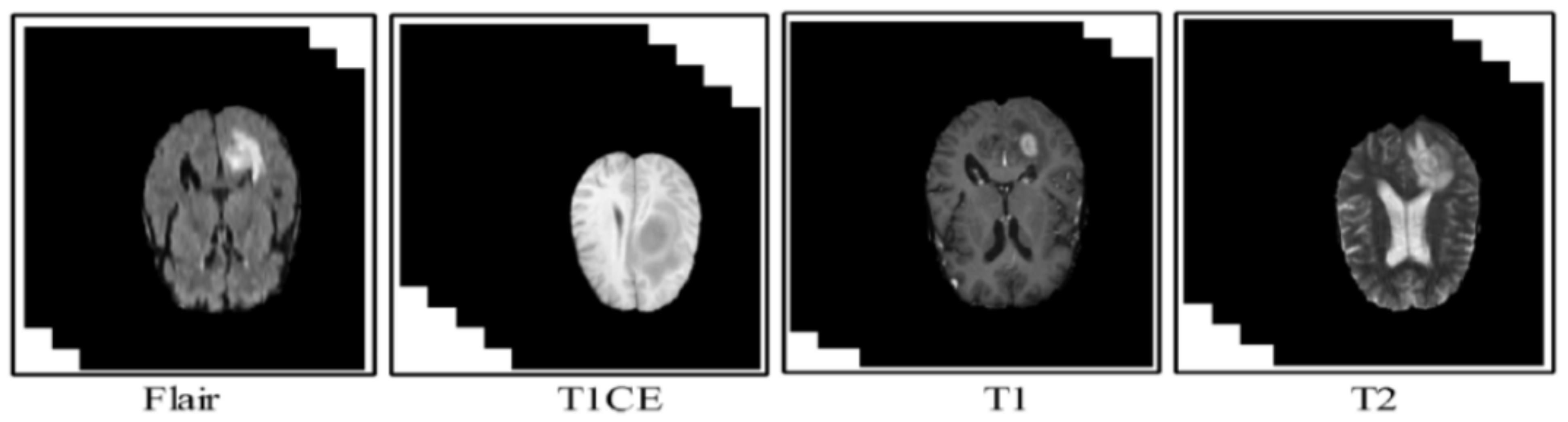
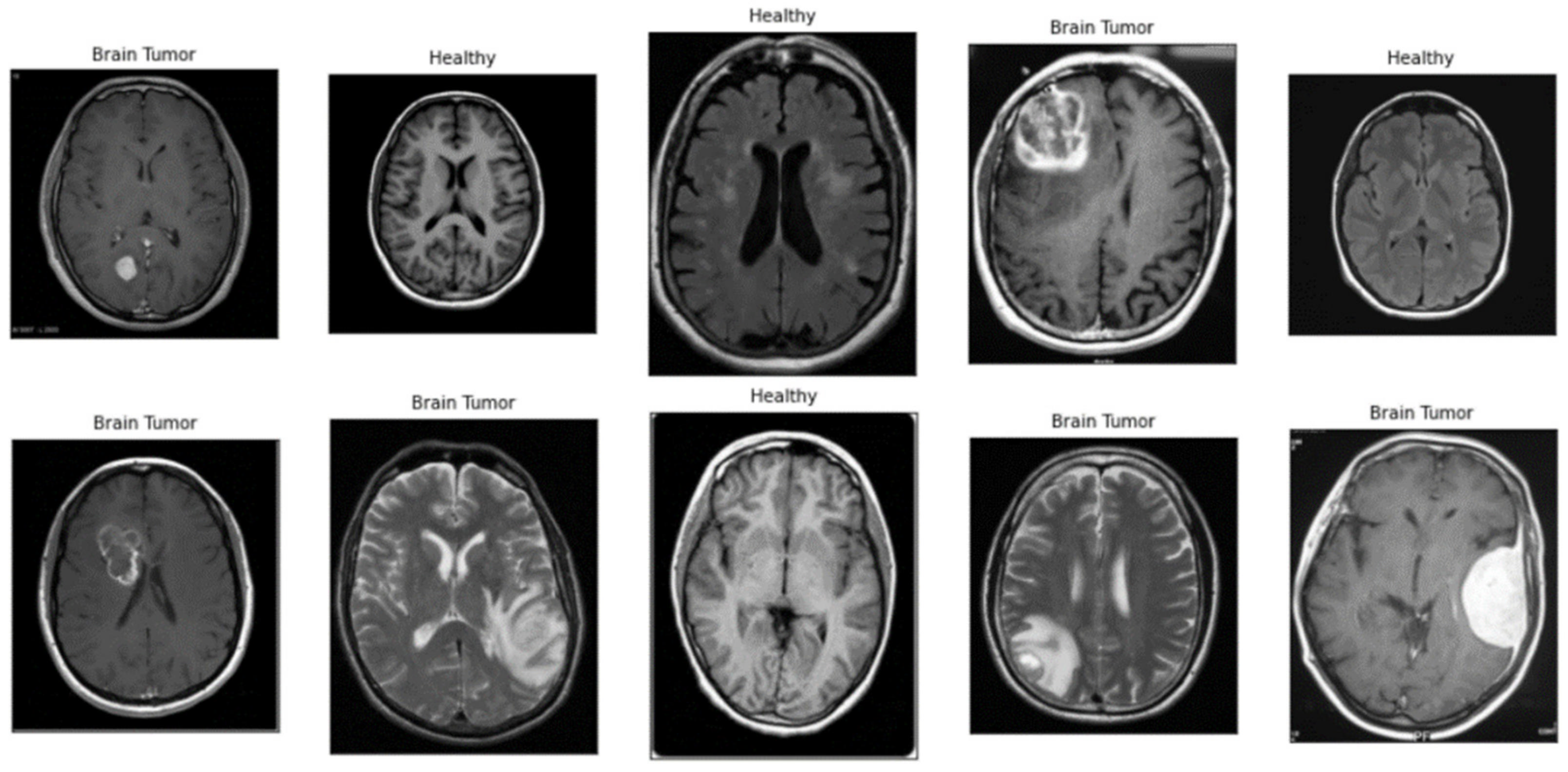
2. Proposed CNN Model in Brain Tumour Dataset

In this analysis, the python code is simulated on the Kaggle platform using TensorFlow, and the optimized “Adam” is chosen for classifying the brain tumours in the whole simulation. Similarly, other python libraries were utilized, such as “numpy”, “pandas”, “time”, “glob”, “matplotlib”, “os”, “cv2” and “shutil” libraries for building the python code and for classifying the considered dataset of brain tumours, where both the healthy and tumour-affected brain magnetic resonance images were presented. The dataset that is considered in this analysis has already undergone a pre-processing phase, with a total of 253 brain MRIs. Out of the 253 brain medical images, 98 images are in the form of a healthy condition and the rest of the 155 images are tumour-affected images [34]. The authors used 20% of the total dataset for testing purposes and the remaining 80% for training the model.

Firstly, the data frame was created with all the images, with the proper directory location in the computer system. The next step was to visualize the images in the Kaggle platform to check the visibility, with figures the size of 16 × 12. Furthermore, the splitting of the data frame was carried out by varying the parameter of the train size over three levels, i.e., 0.85, 0.90 and 0.95. Then, the image data generator operation was performed with a target size of 299 and a batch size of 64, which was kept constant throughout the whole simulation. In the next step, the ResNetV2 model was fitted to the above-mentioned dataset with a zero value for the weights. Furthermore, with the same ResNetV2 model architecture and loading weights, the activation of the “Relu” type function was introduced, with 128 weights in the layers’ dense input. Similarly, for the layers’ dropout input case, a 0.2 constant value was taken, and for the last layers dense input, the “sigmoid” type function was used. In the further step, the above-mentioned CNN model was compiled with the loss and the metrics with varying learning rates, i.e., 0.0001, 0.0002 and 0.0003. Then, the call-back step was carried out with a constant value of the patient as 1, stopping the patient’s value at 3, and with the factor value as 0.5. The training of the prescribed CNN model was carried out with varying epoch numbers, such as 10, 20 and 30. Finally, the predictions of the CNN model were performed where the accuracy value was found to be 1, which meant that the model had 100% accuracy. Lastly, the loss value was computed. Here, the loss value is considered to be the output response for the noble metaheuristic optimization approach. The training loss value should be minimized for the correct classification of the tumour-affected brain MRIs and the healthy ones. Figure 2 shows the simulation images of brain tumours in the Kaggle platform at the optimum setting.

3. Optimization Approaches

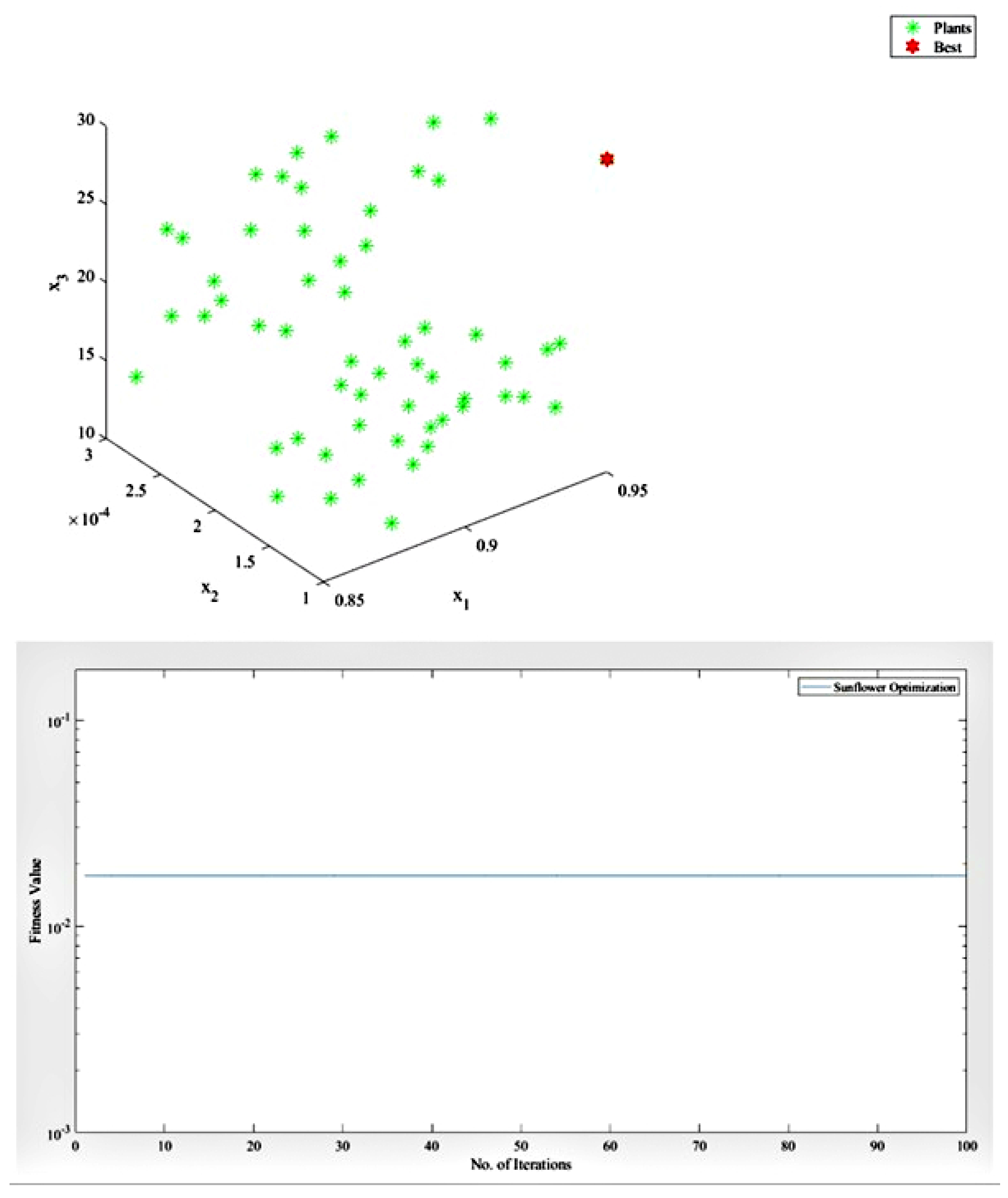
3.1. Sunflower Optimization Algorithm (SFOA)

The life cycle of a sunflower is predictable: as with the needles of a clock, they emerge and accompany the Sun each day. They become the opposite way at night, awaiting the arrival of the Sun the following day’s morning. Another key nature-based optimization is the inverse square law for radiation. Thus, the quantity of heat Q_i absorbed by each plant is computed as follows [36,37]:

$$Q_i=\frac{P}{4\pi r_i^2}$$

(1)

where P indicates the power of the source and r_i denotes the distance between the current supreme and the plant i. The sunflowers’ route to the Sun is defined as follows:

$$\stackrel{\rightharpoonup }{S_i}=\frac{X^{\ast }-X_i}{\parallel X^{\ast }-X_i\parallel },i=1,2,\dots ,n_p$$

(2)

The stride of the sunflowers in the direction “s” is determined as follows:

$$d_i=\lambda \times P_i\left(\parallel X_i-X_{i-1}\parallel \right)\times \parallel X_i-X_{i-1}\parallel$$

(3)

where λ is the perpetual value that denotes a plant’s “inertial” displacement, and $P_i\left(X_i-X_{i-1}\right)$ is the probability of pollination [38].

The maximum step is defined in the following manner:

$$d_{max}=\frac{\parallel X_{max}-X_{min}\parallel }{2\times N_{pop}}$$

(4)

where X_max and X_min denote the maximum and minimum values, respectively, and N_pop denotes the total number of plants.

Within the plant population, the most recent planting would be:

$${\overrightarrow{X}}_{i+1}={\overrightarrow{X}}_i+d_i\times {\overrightarrow{s}}_i$$

(5)

The method begins by generating an even or random population of individuals. The appraisal of each individual permits us to pick which one will be converted into the Sun. Though it is intended to include the potential to function with multiple suns in a future edition, this research is presently constrained to one. After that, similar to sunflowers, all new species will align themselves with the Sun and migrate in a random controlled fashion. Around the Sun, highland plants will pollinate [39]. The SFOA is used find the best solutions to the problem to minimize the fitness function. Sasank and Venkateswarlu [40] used the SFOA to obtain better accuracy when applying the BRATs dataset. They are used the model to increase the accuracy value, not to minimize the training loss.

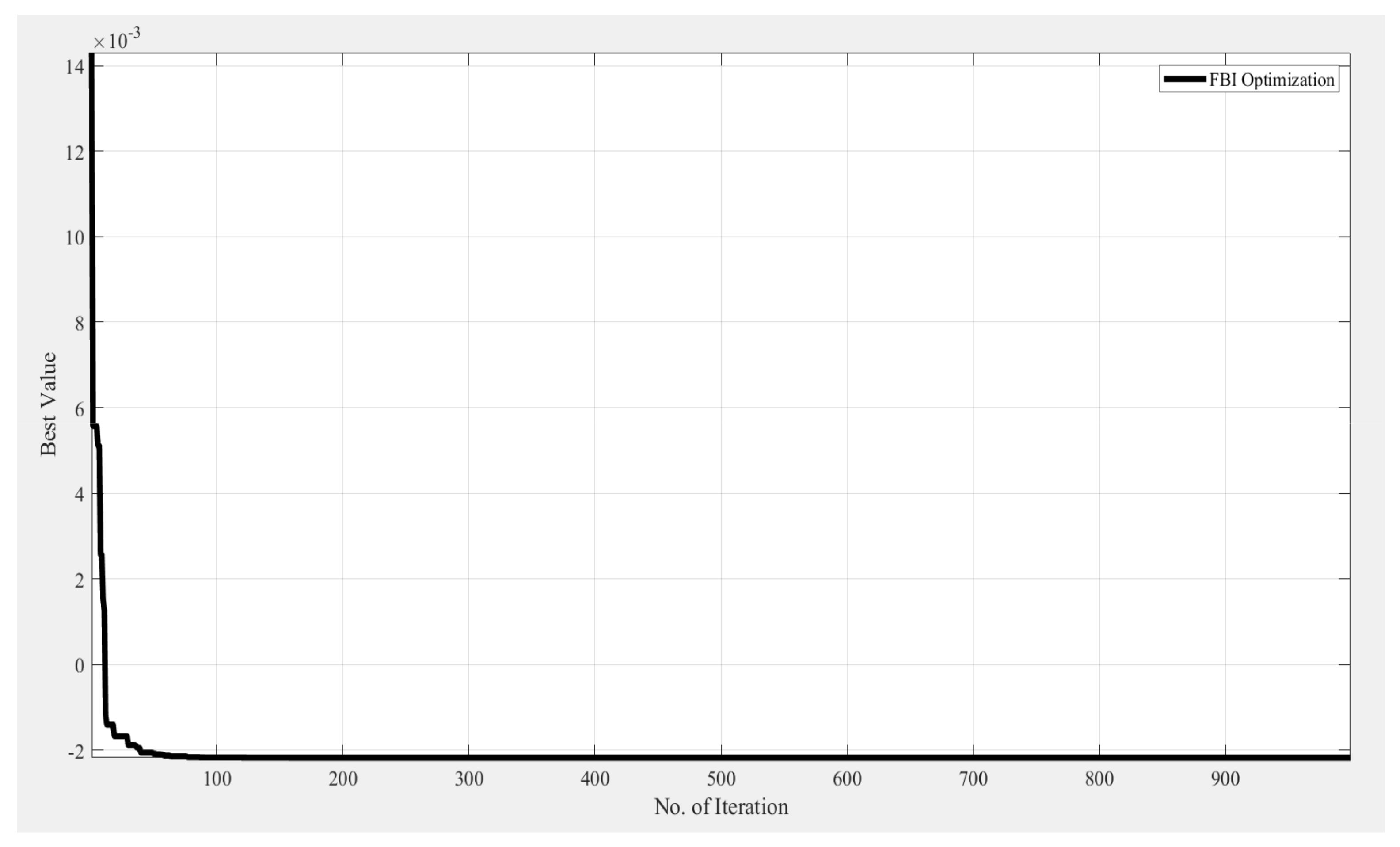
3.2. Forensic-Based Investigation Algorithm (FBIA)

In the year 2020, Chou and Nguyen published the forensic-based investigation algorithm (FBIA), which they developed. It is a metaheuristic optimizer in the traditional sense. Criminals are caught because of the tactics of inquiry, location and stalking that police officers use to apprehend them. This is the primary goal of the FBIA. The following five processes are taken into consideration in a large-scale forensic investigation: case opening, interpretation of results, investigation direction, actions and prosecution [41].

The first phase is for police officers to gather information regarding the crime; this data is then used to direct the investigative team’s efforts. They conduct an investigation into the crime scene, the victim, potential suspects and their prior knowledge of the crime. Additional tasks include locating witnesses and directing their questions to them, as well as conducting the investigation. During the interpretation of results phase, the team examines the information that has been received and attempts to match it with the impressions that have been obtained in order to identify potential suspects. Following that, the investigating team conjures up a criminal situation, reasons for the crime and lines of investigation to go along with the findings. The fourth phase is when the investigation team comes to a conclusion about its findings. In this manner, the truth is accepted through legal accountability [42]. The FBI algorithm is divided into four steps, which are as follows:

Step A1:

This phase is referred to as the “interpretation of findings”, and it is at this stage that the team analyses the data and identifies the first potential suspect’s location. $X_A{}_i$ is used in this phase to determine a new suspected location based on information from previous suspected locations. Equation (6) identifies each individual direction:

$$X_{A1}{}_{ij}=X_{A1}{}_{ij}+\left(\left(ran{d}_1-0.5\right)\ast 2\right)\ast \left(X_A{}_{ij}-\frac{\left(X_A{}_{kj}+X_A{}_{hj}\right)}{2}\right)$$

(6)

where j = 1, 2, ..., D, D is the number of dimensions, ((rand₁ − 0.5) × 2) represents a random number in the range [−1,1], rand₁ is a random number in the range [0,1], k, h, and i are three suspected locations: {k, h, i} ∈ {1, 2, ..., NP}, NP is the number of the population and; k and h are chosen randomly.

Step A2:

This is referred to as the “direction of inquiry”. To determine the most probable suspected location, investigators evaluate the probability of each suspected place to that of other possible sites. P_worst has the lowest probability (the worst objective function value), P_best has the greatest probability (the best objective function value) and X_best is the best location based on the minimization problem. The following Equation (7) has demonstrated probabilities for each location, i.e., Prob($X_A{}_i$):

$$Prob\left(X_{A1}{}_i\right)=\frac{\left(P_{worst}-P_{A_i}\right)}{(P_{worst}-P_{best})}$$

(7)

The best person and other people guide the path of $X_A{}_i$. As with Step A1, Equation (8) updates the new probable location $X_{A2}{}_{ij}$. Then, the value of the objective function (possibility) is determined to determine which one should be updated:

$$X_{A2}{}_{ij}=X_{best}+X_{A_{dj}}+ran{d}_5\ast \left(X_{A_{ej}}+X_{A_{fj}}\right)$$

(8)

where X_best is the updated best position from Step A1, rand₅ is a random number between 0 and 1, d, e, f and i are four possible places: {d, e, f, i} ∈ {1, 2,..., NP} and d, e and f are chosen randomly.

Step B1:

This is the “actions” phase and here, each agent B_i strives to locate the ideal position that has the greatest objective function value (the best option) in regard to Equation (9). If it obtains a more favourable objective function value than the previous site’s ($p_B{}_i$), the newly suggested location is updated:

$$X_{B1}{}_{ij}=ran{d}_{6\ast }{X}_{B_{ij}}+ran{d}_7\ast \left(X_{best}+X_{B_{ij}}\right)$$

(9)

Where X_best is the location that investigators found, rand₆ and rand₇ are two random numbers in the range between 0 and 1 and j = 1, 2,…, D.

Step B2:

This is an expanded version of the “actions” phase. In Step B2, each agent B_i is bound to all other agents in order to establish a new search direction. Agent B_i travels to the finest site and is swayed by the other team members. If $p_B{}_r$ (the probability of agent B_r) is greater than $p_B{}_i$, Equation (10) is used to determine the new position of agent B_i; otherwise, Equation (11) is used:

$$X_{B2}{}_{ij}=X_{B_{rj}}+ran{d}_8\ast (X_{B_{rj}}-X_{B_{ij}})+ran{d}_9\ast \left(X_{best}-X_{B_{rj}}\right)$$

(10)

$$X_{B2}{}_{ij}=X_{B_{rj}}+ran{d}_{10}\ast (X_{B_{ij}}-X_{B_{rj}})+ran{d}_{11}\ast \left(X_{best}-X_{B_{ij}}\right)$$

(11)

where X_best is the best location found in Step B2, rand₈, rand₉, rand₁₀ and rand₁₁ are the random number in the range [0,1], r and i are two police locations: {r, i} ∈ {1, 2,..., NP}, r is chosen randomly and j = 1, 2, …, D [43,44].

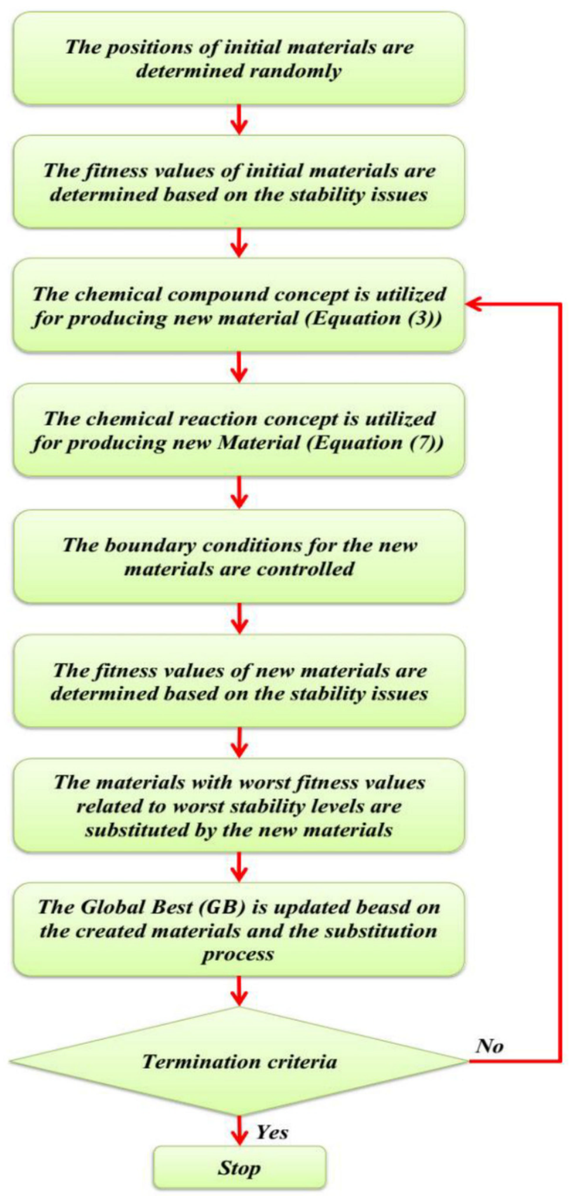
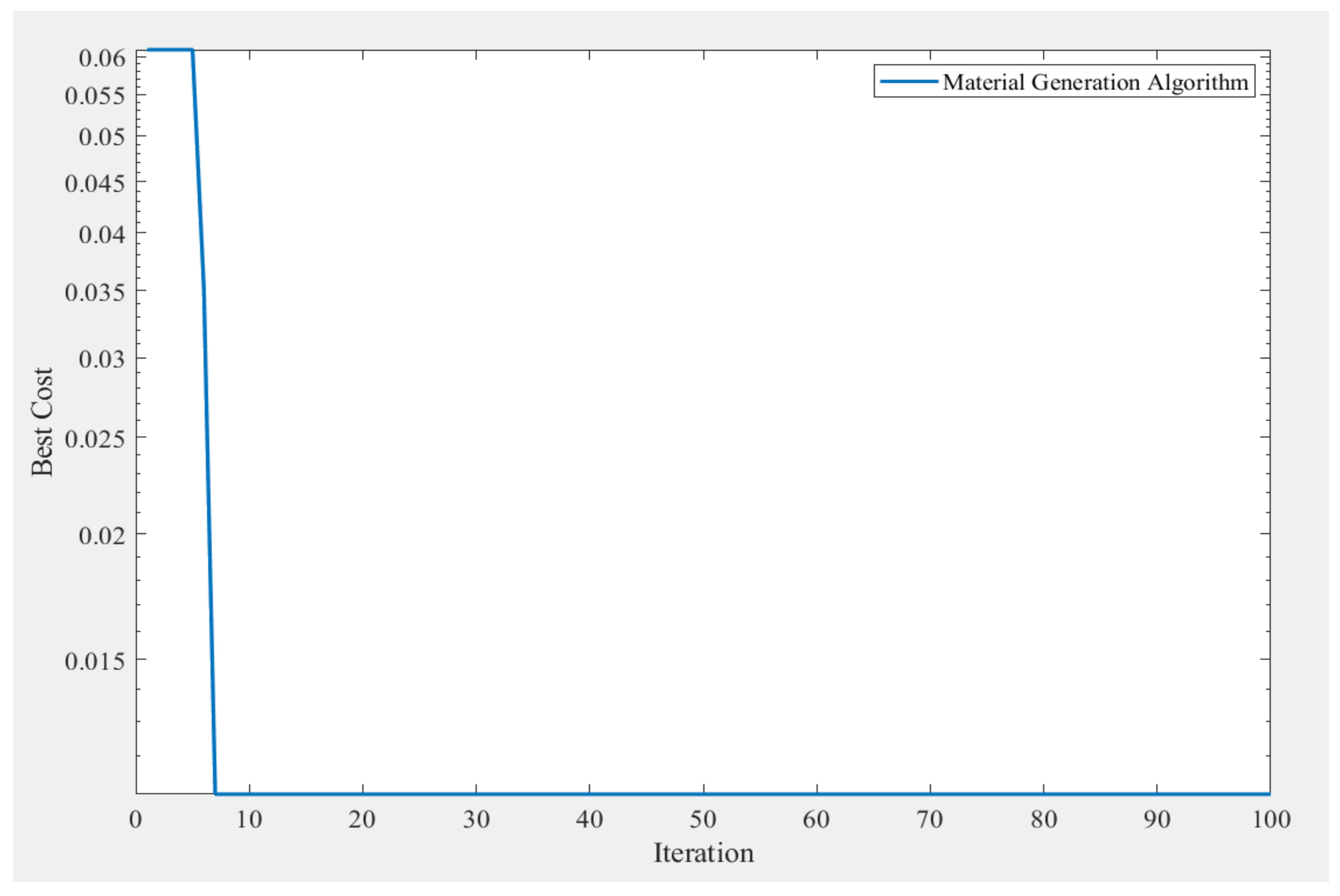
3.3. Material Generation Algorithm (MGA)

The material generation algorithm (MGA) is a revolutionary approach that was developed and is used to assist engineers in generating the best solutions to engineering problems [45]. Some complex and essential aspects of material chemistry, such as the arrangement of chemical molecules and the chemical processes involved in the production of new materials, are thought to be ideas inspired by the MGA.

Inspiration:

Materials are composed of a number of different substances and are made up of the stuff of the cosmos that have both volume and mass. The process of creating new materials entails the possibility for various substances to mix with one another in order to generate new materials with improved functionality and higher energy levels than those that have previously existed. Materials are composed of elements, which are the essential building units that cannot be separated or changed into other elements. Materials are generated at several scales, including the atomic, nano, micro and macro scales, in order to govern their specific properties and improve their performance. A uniquely generated substance is characterized based on its general characteristics and particular characteristics, as well as the physical and chemical changes that have an influence on its behaviour, among other things. When it comes to the material research area, material chemistry ranks as one of the most important subjects to study. Material engineers investigate the configuration of materials in order to increase the unique characteristics of materials, resulting in the development of new materials that are more sustainable and superior to the materials that have previously been developed. Chemical changes in materials are achieved by the reaction of distinct substances with one another and by combining them. In general, the transferring or sharing of electrons between the atoms of different materials has an effect on the chemical properties of the materials. The chemical bonds formed between materials, in particular, are responsible for such transformations. As part of this research, the three essential parts of material chemistry (compounds, reactions and stability) were investigated in order to develop a metaheuristic optimization approach. Figure 3 shows the flowchart of MGA approach which was adopted from its classical theory of the algorithm.

4. Results and Discussion

After obtaining the results of the proposed CNN model, the final outputs, including the accuracy percentage and the training loss, were computed from the nine simulations. The Taguchi L₉ orthogonal design of the experiment, with the training loss output values, is tabulated in

Table 1. Results for training loss using Taguchi’s L₉ orthogonal array.

Sl. No.	Training Size	Learning Rate	No. of Epochs	Training Loss
1	0.85	0.0001	10	0.037515
2	0.85	0.0002	20	0.16
3	0.85	0.0003	30	0.041045
4	0.9	0.0001	20	0.099357
5	0.9	0.0002	30	0.077585
6	0.9	0.0003	10	0.05669
7	0.95	0.0001	30	0.017702
8	0.95	0.0002	10	0.066966
9	0.95	0.0003	20	0.07958

. Furthermore, the above-mentioned nature-inspired algorithms have been applied to optimize the input parameters of the CNN model. The corresponding optimal parametric settings values are tabulated in

Table 2. Results for training loss using Taguchi’s L₉ orthogonal array.

Sl. No.	Proposed Optimization Approaches	Optimal Parametric Setting			Response
		Training Size	Learning Rate	No. of Epochs	Training Loss
1	Sunflower Optimization Algorithm	0.95	0.0001	30	0.017556
2	Forensic-Based Investigation Algorithm	0.85	0.0001	29.99	−0.002174
3	Material Generation Algorithm	0.95	0.0001	30	0.010996

, where the input parameters of the learning rate and the number of epochs were the same value in all three proposed optimization techniques. From this table, it is shown that the maximum value of the train size and the number of epochs and the lowest value of the learning rate gave the minimum value of the output response, i.e., the training loss in the proposed CNN model. The regression model was calculated from the L₉ Taguchi array using MINITAB V20 software and the regression equation with its constraints is given as follows:

Minimize:

$$\begin{gathered} TrainingLoss=\left(-3.730\right)+7.656\ast x\left(1\right)+\left(4494\right)\ast x\left(2\right)+\left(0.01072\right)\ast x\left(3\right) \\ \hspace{1em}\hspace{1em}\hspace{1em}\hspace{1em}\hspace{1em}\hspace{1em}+\left(-4.297\right)\ast x\left(1\right)^2+\left(-5070623\right)\ast x\left(2\right)^2+\left(-0.0007\right) \\ \hspace{1em}\hspace{1em}\hspace{1em}\hspace{1em}\hspace{1em}\ast x\left(3\right)^2+\left(-2647\right)\ast x\left(1\right)\ast x\left(2\right)+0.01802\ast x\left(1\right)\ast x\left(3\right) \end{gathered}$$

(12)

Subject to:

$$0.85\le x\left(1\right)\le 0.95$$

$$0.0001\le x\left(2\right)\le 0.0003$$

$$10\le x\left(3\right)\le 30$$

A set of three sophisticated optimization algorithms are utilized to minimize the output response, i.e., training loss, after nine sets of simulations, and are performed according to the input variables of the CNN model. Three essential input variables with three levels in each are taken into consideration. In this paper, we provide three metaheuristic optimization approaches that were inspired by natural phenomena: the sunflower optimization algorithm, the forensic-based investigation algorithm and the material generation algorithm. When compared to the forensic-based investigation algorithm, only the sunflower optimization algorithm and material generation algorithm approaches have produced the best outcomes out of the three offered strategies. Using both the SFOA and MGA techniques, the optimal values are determined to be 0.95, 0.0001 and 30 for the training size, learning rate and number of epochs, respectively, for the three parameters. However, in the instance of the FBIA method, the optimal setting is found to be 0.85, 0.0001 and 29.99 for all the input variables, and the output response value becomes negative, indicating that the output response is not achievable in this scenario. According to Table 1, it can be seen that the lowest value for the training loss occurs during the seventh run. Furthermore, the comparative study of the three suggested algorithms with the optimal parameters and output response value is shown in Table 2.

Figure 4 depicts the convergence plot of the sunflower optimization algorithm, which demonstrates the best fitness function value for the training loss output based on the best fitness function value, and which also represents the obtained best optimum fitness value. For the same reason, Figure 5 illustrates the findings of the forensic-based investigation algorithm approach and, lastly, Figure 6 depicts the results of the material generation algorithm approach for the CNN model of brain tumours, which yielded an accuracy value of 100%.

Tumour cell categorization is challenging due to their diverse nature. Convolutional neural networks (CNN) are the most widely used machine learning method for visual learning and brain tumour recognition. This study proposes a CNN model for brain tumour magnetic resonance imaging, as well as parametric optimization methodologies. Throughout the nine runs, i.e., Taguchi’s L9 design of experiment, the accuracy percentage in the simulation of the above-described model is exactly 100 percent. Readers interested in applying these strategies to a range of technological and medical difficulties will be interested in this comparative examination of all three algorithms. We have used new sophisticated optimization techniques, such as SFOA, FBIA and MGA, to optimize the parameters of a convolutional neural network approach that is applied to a dataset of brain MRIs to detect any area affected by tumours. Each algorithm comes with its own set of benefits and drawbacks. We compared all three proposed algorithms for our study in order to find the most optimal solution possible because the results of the optimum fitness value change slightly throughout the analysis when determining the most appropriate parameters of the prescribed CNN model for the classification of brain MRIs. Out of the three optimization techniques, the forensic-based investigation algorithm gave negative values for the output response, so this method does not fit the considered dataset. In the case of the other techniques, i.e., the sunflower optimization algorithm and the material generation algorithm, they functioned well for the entirety of the simulations using the brain tumour MRIs dataset with the proposed CNN model.

5. Conclusions

In this study, a novel 3D deep learning supervised ResNetV2 model is employed to identify brain tumours in multi-modal magnetic resonance pictures. With the aim of minimizing the training loss during the output response of the model when applied to the brain tumour dataset, the sunflower optimization algorithm (SFOA), the forensic-based investigation algorithm (FBIA) and the material generation algorithm (MGA) have been introduced to classify the tumours in the whole dataset. The output results are compared with proposed optimization techniques along with the previously reported state-of-the-art of CNNs in the field of brain tumour classification. In clinical trials for the exact diagnosis and improved treatment management of brain tumours, and similar medical conditions where magnetic resonance images are used, the implementation of the specified framework will be a major contribution, with its high classification accuracy and little training loss, which is the main research problem nowadays. Lastly, the sunflower optimization and material generation algorithms have shown better results than the forensic-based investigation algorithm in this CNN model of brain tumour classification. There is scope in other types of work for advanced bio-inspired optimization, as in this CNN model for classifying tumours in the brain MRIs dataset. Moreover, there will be a scope to implement and use advanced deep learning techniques to improve the identification of tumours in the brain, as well as other medical fields where image processing has been carried out.

References

1. Gondal, A.H.; Khan, M.N.A. A Review of Fully Automated Techniques for Brain Tumor Detection from MR Images. Int. J. Mod. Educ. Comput. Sci. Rev. 2013, 5, 55. [Google Scholar] [CrossRef]
2. Iftekharuddin, K.M. Techniques in Fractal Analysis and Their Applications in Brain MRI. Med. Imaging Syst. Technol. Anal. Comput. Methods World Sci. 2005, 1, 63–86. [Google Scholar]
3. Wang, D.; Doddrell, D. A Segmentation-Based and Partial-Volume-Compensated Method for an Accurate Measurement of Lateral Ventricular Volumes on T1-Weighted Magnetic Resonance Images. Magn. Reson. Imaging 2001, 19, 267–273. [Google Scholar] [CrossRef]
4. Krishnamurthy, A.K.; Ahalt, S.C.; Melton, D.E.; Chen, P. Neural Networks for Vector Quantization of Speech and Images. IEEE J. Select. Areas Commun. 1990, 8, 1449–1457. [Google Scholar] [CrossRef]
5. Zhao, X.; Wu, Y.; Song, G.; Li, Z.; Zhang, Y.; Fan, Y. A Deep Learning Model Integrating FCNNs and CRFs for Brain Tumor Segmentation. Med. Image Anal. 2018, 43, 98–111. [Google Scholar] [CrossRef]
6. Wang, G.; Zuluaga, M.A.; Pratt, R.; Aertsen, M.; Doel, T.; Klusmann, M.; David, A.L.; Deprest, J.; Vercauteren, T.; Ourselin, S. Slic-Seg: A Minimally Interactive Segmentation of the Placenta from Sparse and Motion-Corrupted Fetal MRI in Multiple Views. Med. Image Anal. 2016, 34, 137–147. [Google Scholar] [CrossRef]
7. Top, A.; Hamarneh, G.; Abugharbieh, R. Active Learning for Interactive 3D Image Segmentation. In Proceedings of the International Conference on Medical Image Computing and Computer-Assisted Intervention, Toronto, ON, Canada, 18–22 September 2011; Springer: Berlin/Heidelberg, Germany, 2011; pp. 603–610. [Google Scholar]
8. Rother, C.; Kolmogorov, V.; Blake, A. “GrabCut” Interactive Foreground Extraction Using Iterated Graph Cuts. ACM Trans. Gr. 2004, 23, 309–314. [Google Scholar] [CrossRef]
9. Havaei, M.; Davy, A.; Warde-Farley, D.; Biard, A.; Courville, A.; Bengio, Y.; Pal, C.; Jodoin, P.M.; Larochelle, H. Brain Tumor Segmentation with Deep Neural Networks. Med. Image Anal. 2017, 35, 18–31. [Google Scholar] [CrossRef] [PubMed]
10. Bauer, S.; Wiest, R.; Nolte, L.-P.; Reyes, M. A Survey of MRI-Based Medical Image Analysis for Brain Tumor Studies. Phys. Med. Biol. 2013, 58, R97. [Google Scholar] [CrossRef]
11. Rehman, A.; Khan, M.A.; Saba, T.; Mehmood, Z.; Tariq, U.; Ayesha, N. Microscopic Brain Tumor Detection and Classification Using 3D CNN and Feature Selection Architecture. Microsc. Res. Tech. 2021, 84, 133–149. [Google Scholar] [CrossRef] [PubMed]
12. Reza, S.; Iftekharuddin, K. Improved Brain Tumor Tissue Segmentation Using Texture Features. Proc. MICCAI BraTS 2014, 10134, 27–30. [Google Scholar]
13. Goetz, M.; Weber, C.; Bloecher, J.; Stieltjes, B.; Meinzer, H.-P.; Maier-Hein, K. Extremely Randomized Trees Based Brain Tumor Segmentation. In Proceedings of the BRATS Challange-MICCAI, Boston, MA, USA, 14 September 2014; pp. 006–011. [Google Scholar]
14. Kleesiek, J.; Biller, A.; Urban, G.; Kothe, U.; Bendszus, M.; Hamprecht, F. Ilastik for Multi-Modal Brain Tumor Segmentation. Proc. MICCAI BraTS 2014, 12–17. [Google Scholar]
15. Sarhan, A.M. Brain Tumor Classification in Magnetic Resonance Images Using Deep Learning and Wavelet Transform. J. Biomed. Sci. Eng. Appl. Artif. Intell. 2020, 13, 102. [Google Scholar] [CrossRef]
16. Siar, M.; Teshnehlab, M. Brain Tumor Detection Using Deep Neural Network and Machine Learning Algorithm. In Proceedings of the 2019 9th International Conference on Computer and Knowledge Engineering (ICCKE), Mashhad, Iran, 24–25 October 2019; pp. 363–368. [Google Scholar]
17. Roy, S.; Bandyopadhyay, S.K. Detection and Quantification of Brain Tumor from MRI of Brain and Its Symmetric Analysis. Int. J. Inform. Commun. Technol. Res. 2012, 2, 477–483. [Google Scholar]
18. Mittal, M.; Goyal, L.M.; Kaur, S.; Kaur, I.; Verma, A.; Hemanth, D.J. Deep Learning Based Enhanced Tumor Segmentation Approach for MR Brain Images. Appl. Soft Comput. 2019, 78, 346–354. [Google Scholar] [CrossRef]
19. Raja, P.S. Brain Tumor Classification Using a Hybrid Deep Autoencoder with Bayesian Fuzzy Clustering-Based Segmentation Approach. Biocybern. Biomed. Eng. 2020, 40, 440–453. [Google Scholar] [CrossRef]
20. Mustaqeem, A.; Javed, A.; Fatima, T. An Efficient Brain Tumor Detection Algorithm Using Watershed & Thresholding Based Segmentation. Int. J. Image Gr. Signal Process. 2012, 4, 34. [Google Scholar]
21. Vaidhya, K.; Thirunavukkarasu, S.; Alex, V.; Krishnamurthi, G. Multi-Modal Brain Tumor Segmentation Using Stacked Denoising Autoencoders. In BrainLes 2015; Springer: Berlin/Heidelberg, Germany, 2015; pp. 181–194. [Google Scholar]
22. Agn, M.; Puonti, O.; af Rosenschöld, P.M.; Law, I.; Van Leemput, K. Brain Tumor Segmentation Using a Generative Model with an RBM Prior on Tumor Shape. In BrainLes 2015; Springer: Berlin/Heidelberg, Germany, 2015; pp. 168–180. [Google Scholar]
23. Jia, Z.; Chen, D. Brain Tumor Identification and Classification of MRI Images Using Deep Learning Techniques. IEEE Access 2020, 1–10. [Google Scholar] [CrossRef]
24. Mahalakshmi, S.; Velmurugan, T. Detection of Brain Tumor by Particle Swarm Optimization Using Image Segmentation. Indian J. Sci. Technol. 2015, 8, 1. [Google Scholar] [CrossRef]
25. Mansour, R.F.; Escorcia-Gutierrez, J.; Gamarra, M.; Díaz, V.G.; Gupta, D.; Kumar, S. Artificial Intelligence with Big Data Analytics-Based Brain Intracranial Hemorrhage E-Diagnosis Using CT Images. Neural Comput. Appl. 2021, 1–17. [Google Scholar] [CrossRef]
26. Reddy, A.V.N.; Krishna, C.P.; Mallick, P.K.; Satapathy, S.K.; Tiwari, P.; Zymbler, M.; Kumar, S. Analyzing MRI Scans to Detect Glioblastoma Tumor Using Hybrid Deep Belief Networks. J. Big Data 2020, 7, 1–17. [Google Scholar] [CrossRef]
27. Havaei, M.; Dutil, F.; Pal, C.; Larochelle, H.; Jodoin, P.-M. A Convolutional Neural Network Approach to Brain Tumor Segmentation. In BrainLes 2015; Springer: Berlin/Heidelberg, Germany, 2015; pp. 195–208. [Google Scholar]
28. Pradhan, A.; Mishra, D.; Das, K.; Panda, G.; Kumar, S.; Zymbler, M. On the Classification of MR Images Using “ELM-SSA” Coated Hybrid Model. Mathematics 2021, 9, 2095. [Google Scholar] [CrossRef]
29. Kamnitsas, K.; Ledig, C.; Newcombe, V.F.; Simpson, J.P.; Kane, A.D.; Menon, D.K.; Rueckert, D.; Glocker, B. Efficient Multi-Scale 3D CNN with Fully Connected CRF for Accurate Brain Lesion Segmentation. Med. Image Anal. 2017, 36, 61–78. [Google Scholar] [CrossRef] [PubMed]
30. Yi, D.; Zhou, M.; Chen, Z.; Gevaert, O. 3-D Convolutional Neural Networks for Glioblastoma Segmentation. arXiv 2016, arXiv:1611.04534v1. [Google Scholar]
31. El-Dahshan, E.-S.A.; Mohsen, H.M.; Revett, K.; Salem, A.-B.M. Computer-Aided Diagnosis of Human Brain Tumor through MRI: A Survey and a New Algorithm. Expert Syst. Appl. 2014, 41, 5526–5545. [Google Scholar] [CrossRef]
32. Dong, H.; Yang, G.; Liu, F.; Mo, Y.; Guo, Y. Automatic Brain Tumor Detection and Segmentation Using U-Net Based Fully Convolutional Networks. In Medical Image Understanding and Analysis. MIUA 2017; Valdés Hernández, M., González-Castro, V., Eds.; Springer: Cham, Switzerland, 2017. [Google Scholar] [CrossRef]
33. Padole, V.B.; Chaudhari, D. Detection of Brain Tumor in MRI Images Using Mean Shift Algorithm and Normalized Cut Method. Int. J. Eng. Adv. Technol. 2012, 1, 53–56. [Google Scholar]
34. Brain MRI Images for Brain Tumor Detection. 2019. Available online: https://www.kaggle.com/navoneel/brain-mri-images-for-brain-tumor-detection (accessed on 12 October 2021).
35. Brain MRI Image 100% Accuracy. 2021. Available online: https://www.kaggle.com/code/vexxingbanana/brain-mri-image-100-accuracy/notebook (accessed on 12 October 2021).
36. Gomes, G.F.; Giovani, R.S. An efficient Two-Step Damage Identification Method Using Sunflower Optimization Algorithm and Mode Shape Curvature (MSDBI–SFO). Eng. Comput. 2020, 1–20. [Google Scholar] [CrossRef]
37. Francisco, M.B.; Pereira, J.L.J.; Oliver, G.A.; da Silva, F.H.S.; da Cunha, S.S., Jr.; Gomes, G.F. Multiobjective Design Optimization of CFRP Isogrid Tubes Using Sunflower Optimization Based on Metamodel. Comput. Struct. 2021, 249, 106508. [Google Scholar] [CrossRef]
38. El-Sehiemy, R.A.; Hamida, M.A.; Mesbahi, T. Parameter Identification and State-of-Charge Estimation for Lithium-Polymer Battery Cells Using Enhanced Sunflower Optimization Algorithm. Int. J. Hydrog. Energy 2020, 45, 8833–8842. [Google Scholar] [CrossRef]
39. Qais, M.H.; Hasanien, H.M.; Alghuwainem, S. Identification of Electrical Parameters for Three-Diode Photovoltaic Model Using Analytical and Sunflower Optimization Algorithm. Appl. Energy 2019, 250, 109–117. [Google Scholar] [CrossRef]
40. Sasank, V.V.S.; Vankateswarlu, S. An Automatic Tumour Growth Prediction Based Segmentation Using Full Resolution Convolutional Network for Brain Tumour. Biomed. Signal Process. Control 2022, 71, 103090. [Google Scholar] [CrossRef]
41. Chou, J.S.; Nguyen, N.M. FBI Inspired Meta-Optimization. Appl. Soft Comput. 2020, 93, 106339. [Google Scholar] [CrossRef]
42. Kuyu, Y.Ç.; Vatansever, F. Modified Forensic-Based Investigation Algorithm for Global Optimization. Eng. Comput. 2021, 1–22. [Google Scholar] [CrossRef]
43. Shaheen, A.M.; Ginidi, A.R.; El-Sehiemy, R.A.; Ghoneim, S.S. A Forensic-Based Investigation Algorithm for Parameter Extraction of Solar Cell Models. IEEE Access 2020, 9, 1–20. [Google Scholar] [CrossRef]
44. Fathy, A.; Rezk, H.; Alanazi, T.M. Recent Approach of Forensic-Based Investigation Algorithm for Optimizing Fractional Order PID-Based MPPT with Proton Exchange Membrane Fuel Cell. IEEE Access 2021, 9, 18974–18992. [Google Scholar] [CrossRef]
45. Talatahari, S.; Azizi, M.; Gandomi, A.H. Material Generation Algorithm: A Novel Metaheuristic Algorithm for Optimization of Engineering Problems. Processes 2021, 9, 859. [Google Scholar] [CrossRef]
Figure 1. Different types of brain tumour [11].
Computers 11 00010 g001
Figure 2. Simulation images of brain tumours in the Kaggle platform [35].
Computers 11 00010 g002
Figure 3. Flowchart of the material generation algorithm [45].
Computers 11 00010 g003
Figure 4. Result of the sunflower optimization approach.
Computers 11 00010 g004
Figure 5. Result of the forensic-based investigation algorithm approach.
Computers 11 00010 g005
Figure 6. Result of the material generation algorithm approach.
Computers 11 00010 g006