
A Transfer-Learning-Based Novel Convolution Neural Network for Melanoma Classification


1
Electrical Engineering Section, University Polytechnic, Aligarh Muslim University, Aligarh 202001, India
2
Department of Computer Engineering, Zakir Hussain College of Engineering & Technology, Aligarh Muslim University, Aligarh 202001, India
3
Department of Business Administration, College of Business Administration, Princess Nourah Bint Abdulrahman University, P.O. Box 84428, Riyadh 11671, Saudi Arabia
*
Author to whom correspondence should be addressed.
Computers 2022, 11(5), 64; https://0-doi-org.brum.beds.ac.uk/10.3390/computers11050064
Submission received: 21 March 2022
/
Revised: 20 April 2022
/
Accepted: 20 April 2022
/
Published: 26 April 2022
(This article belongs to the Special Issue Advances of Machine and Deep Learning in the Health Domain)
Abstract
:Skin cancer is one of the most common human malignancies, which is generally diagnosed by screening and dermoscopic analysis followed by histopathological assessment and biopsy. Deep-learning-based methods have been proposed for skin lesion classification in the last few years. The major drawback of all methods is that they require a considerable amount of training data, which poses a challenge for classifying medical images as limited datasets are available. The problem can be tackled through transfer learning, in which a model pre-trained on a huge dataset is utilized and fine-tuned as per the problem domain. This paper proposes a new Convolution neural network architecture to classify skin lesions into two classes: benign and malignant. The Google Xception model is used as a base model on top of which new layers are added and then fine-tuned. The model is optimized using various optimizers to achieve the maximum possible performance gain for the classifier output. The results on ISIC archive data for the model achieved the highest training accuracy of 99.78% using Adam and LazyAdam optimizers, validation and test accuracy of 97.94% and 96.8% using RMSProp, and on the HAM10000 dataset utilizing the RMSProp optimizer, the model achieved the highest training and prediction accuracy of 98.81% and 91.54% respectively, when compared to other models.
1. Introduction
Melanoma skin cancers, including other categories of non-melanoma, are increasing globally. In the US alone, it is estimated that 99,780 new melanomas will be diagnosed in 2022, and around 7650 people are expected to die of malignant melanoma. Melanoma is more common in white people compared to African Americans. Overall, 1 in 38 are at lifetime risk of getting melanoma for white people, while it is 1 in 1000 for black people and 1 in 167 for Hispanics. Despite new therapeutic agents, such as checkpoint and BRAF inhibitors, to improve the survival of cases in advanced stages, melanomas still become fatal [1]. It is the most harmful type of skin cancer, which causes pigmented marks on the skin in humans [2]. The abnormality in the melanin-producing cells, also called melanocytes, is the main reason for melanoma. Certain risk factors are associated with melanomas, such as fair skin, hereditary factors, sunburn history, weakened immune system, exposure to ultraviolet light, and the use of tanning beds. Melanoma, if diagnosed in later stages, has a survival rate below 14%. However, if it is detected in the early stages, the survival rate is around 97% [3]. Thus, it is paramount that melanoma skin cancer is detected early with improved accuracy to increase survival. A skilled dermatologist generally goes through steps, starting with the observation of the suspected lesions, then dermoscopy by magnifying the lesions using a microscope and finally a biopsy [4]. It is a time-consuming and low-accuracy process that further leads the patient to later stages. It is also found that under 80% of dermatologist diagnoses are correctly diagnosing the skin cancer with this process [5]. To overcome all these problems, a lot of algorithmic solutions are developed using computerized image analysis techniques [6]. Most of the developed solutions are parametric, which requires the data to be distributed normally. As the dataset is heterogeneous, it would be insufficient to diagnose the disease accurately with these methods.
Convolution neural networks (CNNs) that are part of deep neural networks (DNNs) are far better than other methods for performing tasks, such as object detection and image classification [7]. Significant research has been conducted in the field of natural image classification, and these works have produced CNN architecture such as GoogLeNet [8], AlexNet [9], ResNet [10], VGGNet [11] and others. These architectures can be used as pre-trained models that are publicly available. They were initially trained on around 1.28 million natural images of 1000 classes from the ImageNet dataset [12]. Other models can use the weights and biases from these pre-trained models. It means that by fine-tuning all the layers or some specific layers of these models using backpropagation using our dataset, they can be used in the proposed task of skin cancer classification.
The weights and biases of AlexNet and VGGNet are initialized because the visual information may differ from skin images. In medical image analysis, access to validated data is expensive and heavily restricted, due to which training of CNNs from scratch becomes a tedious task [13]. The transfer learning approach can overcome this problem because it uses a pre-trained network (i.e., one trained on other types of images rather than domain-specific) and adapts it to the classification problem at hand. Valuable features are identified by using this pre-trained model even when the training samples are limited [14]. Recently, medical image analysis in different applications, such as cardiology, diabetic retinopathy, radiology, ultrasound imaging, gastroenterology, breast cancer diagnosis, microscopic imaging and dermoscopy, has used transfer learning [15]. Two different transfer learning techniques have been used for skin lesion classification. In one of the techniques, a pre-trained CNN is used to generate features. Here, images are given as input to the pre-trained CNN model, and then features are extracted from a convolution layer or a particular fully connected (FC) layer [16]. A classifier such as SVM can be built using these extracted features [17]. These extracted features were encoded to discriminative and more invariant representations, and to increase classification performance, they are consolidated with other hand-crafted feature descriptors. The second technique used in transfer learning is that the pre-trained models can be adapted to the other domain or problem by fine-tuning the network layers. In the work proposed in [18], the fully connected or FC layers of the pre-trained model were replaced by more new layers, and then the re-training of the model was conducted so that the weights of the newly added layers could be adapted for the classification of skin lesions. In different research work conducted so far, the pre-trained models that are used in both transfer learning techniques for skin lesion classification varied differently, including VGG16, VGG19, ResNet-152 and Inception-v4 [19].
Recently, some research work is also carried out for melanoma detection using autoencoders. In the work published in [20], stacked sparse autoencoders are used to discover pixel intensities from the input images, which are high-level features given as input to the classifier. Here, instead of training the whole network at once like in CNN, each layer is trained separately, and then fine-tuning of the network is conducted to improve the performance. Here, the authors also proposed a novel deep neural network architecture based on the bag-of-features (BOF) model, which represents an image as a set of independent local descriptors, and these are then quantized in the form of a histogram vector. Color features are also included in local descriptors to better classify the input skin lesion image. Here, the SIFT (Scale Invariant Feature Transform) [21] descriptor is combined with color information. The proposed method achieved an accuracy of 95%, specificity value of 94.9% and sensitivity value of 95.4% using BOF input to deep autoencoder instead of raw images. Recently, a case-based reasoning (CBR) system was proposed in [22] to support users in obtaining the image of affected skin area. The ISIC archive dataset is utilized in the analysis of skin lesion classification as a benign and malignant melanoma. The kernel of the CBR system is built upon a CNN with sixteen layers that trained and learned recursively. The proposed work gives an accuracy of only 75% on the ISIC archive dataset.
Although many methods have been developed for melanoma screening, a systematic approach is missing, and the models proposed so far are too complex. Additionally, the results of some important metrics in the medical images classification domain, such as specificity and sensitivity, are not up to the mark.
Thus, to overcome these shortcomings, a novel CNN model is proposed using a transfer learning approach to assist the dermatologist in accurately diagnosing skin cancer.
2. Material and Methods
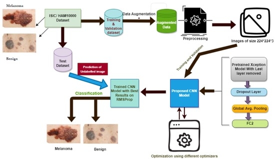
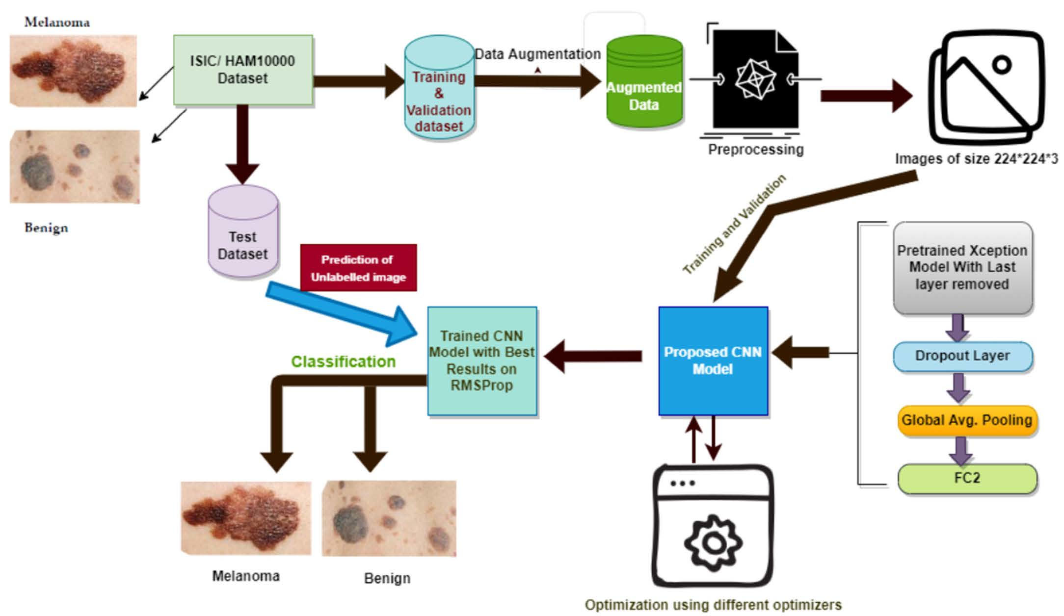
This research aims to develop the best transfer learning approach to classify skin lesion images into two classes. The first class is benign skin tumors, and the second class is malignant cancerous melanoma. The method proposed in this work has the following workflow:
- Dataset selection and augmentation: ISIC archive dataset is selected, and data augmentation is applied to overcome the class imbalance problem, leading to overfitting;
- Preprocessing: Input image preprocessing is kept minimum to increase the generalization ability and adaptability of the proposed model for other classification tasks;
- Selection of base model: Xception model [23], a well-known CNN model pre-trained on the ImageNet dataset, is selected as the base model;
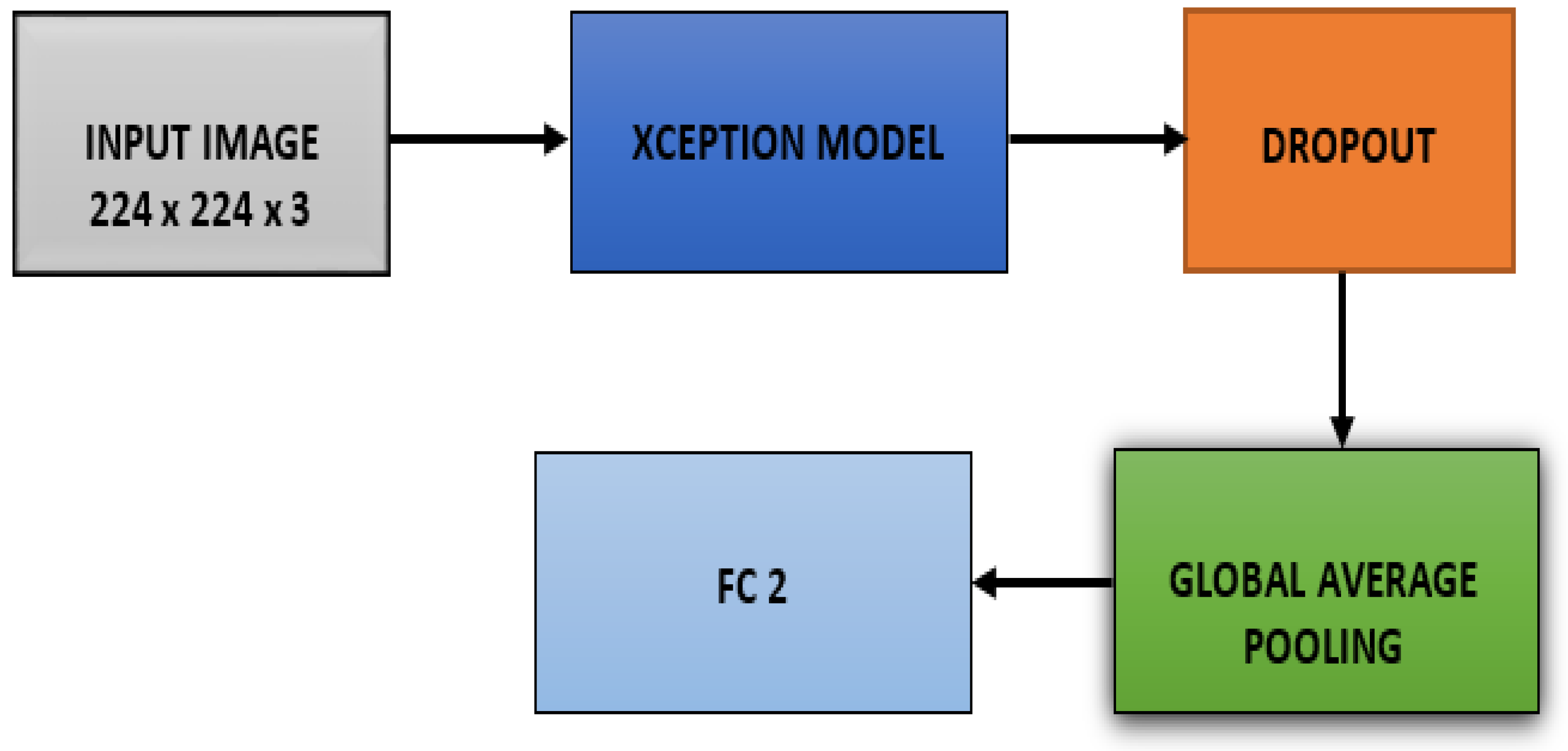
- The last layer of the Xception model is removed, and three more layers are added: drop out layer, global average pooling, and dense or FC layer with two nodes, which is the last layer for binary classification, i.e., melanoma or benign;
- The pre-trained Xception network is fine-tuned multiple times on the ISIC archive dataset with different settings to achieve more accuracy and good performance for skin lesion classification;
- The model is optimized using six different optimizers, and the model performance is compared on each of those optimizers;
- A novel variable learning rate algorithm and early stopping criterion are used to avoid unnecessary model training for fix number of epochs;
- Results: The proposed method’s performance in every different setting is shown and compared to other techniques developed so far.
- Figure 1 below shows the steps that are followed in the proposed methodology.
The following subsections give detailed descriptions of each stage of our proposed methodology.
2.1. Dataset and Its Augmentation
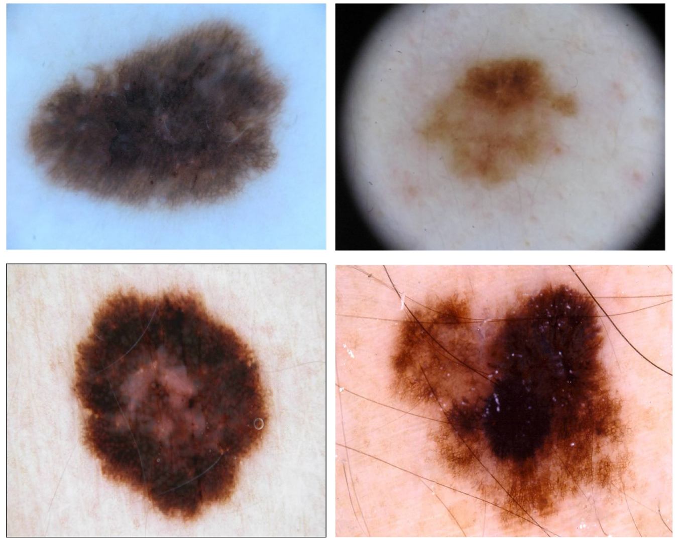
The ISIC archive dataset is used in this study, which consists of publicly available images of skin lesions under Creative Commons licenses. There are over 150,000 images in the ISIC archive, of which approximately 70,000 have been made public. There are many classes of skin lesion images in the ISIC archive with ground-truth diagnoses and other clinical metadata. These images are contributions from specialized melanoma centers from around the world [24]. For the proposed work, two classes, i.e., benign and melanoma, of images were taken from the ISIC archive. The number of images downloaded for benign was 5000 and for that of melanoma was 2285, out of which 10% of images were taken for testing purposes, i.e., 500 and 228 from each class. Therefore, the number of images left for training and validation purposes of the benign class is 4500 and 2057 for melanoma. Here, one thing to note is that there is a class imbalance both in the test and training and validation datasets, which will result in a model that may have low performance on the test dataset, specifically for the minority class.
To overcome this, data augmentation [25] is used to make the number of samples for each class equal for both training and test data. There are several ways for data augmentation; we have rotated the image at an angle of 180°, image width and height shift by a factor of 0.05 each, zoom shift by 0.05 and horizontal and vertical flip set to true. Using these transformations, 272 images were generated for the test set from the melanoma class and 2443 for the training dataset from the melanoma class, making each class’s contribution equal to the training and test datasets. Afterwards, the total number of images in the training dataset is 9000, and 33 % are taken for the validation set, 2970, and the remaining 6030 for the training part. Finally, the test dataset contains 1000 images of melanoma and benign tumors. The sample images from each class in the ISIC dataset is shown in the Figure 2 below.
2.2. Preprocessing
The preprocessing steps in the proposed work are very few to support the model’s generalization ability when tested on other datasets. The original images are 1022 by 767, which are resized to 224 × 224 × 3, i.e., height, width and depth. All the images are scaled down by a rescaling factor of 255 before giving input to the model. The dataset consists of a colorful image that contains three maps: Red, Green and Blue. All the pixels are in the range of 0–255, and these values would be too high for our model to process, so rescaling by a factor of 1/255 transforms all pixels’ value in the range of 0–1 [26].
2.3. Pre-Trained Convolution Neural Network Model and Its Fine-Tuning
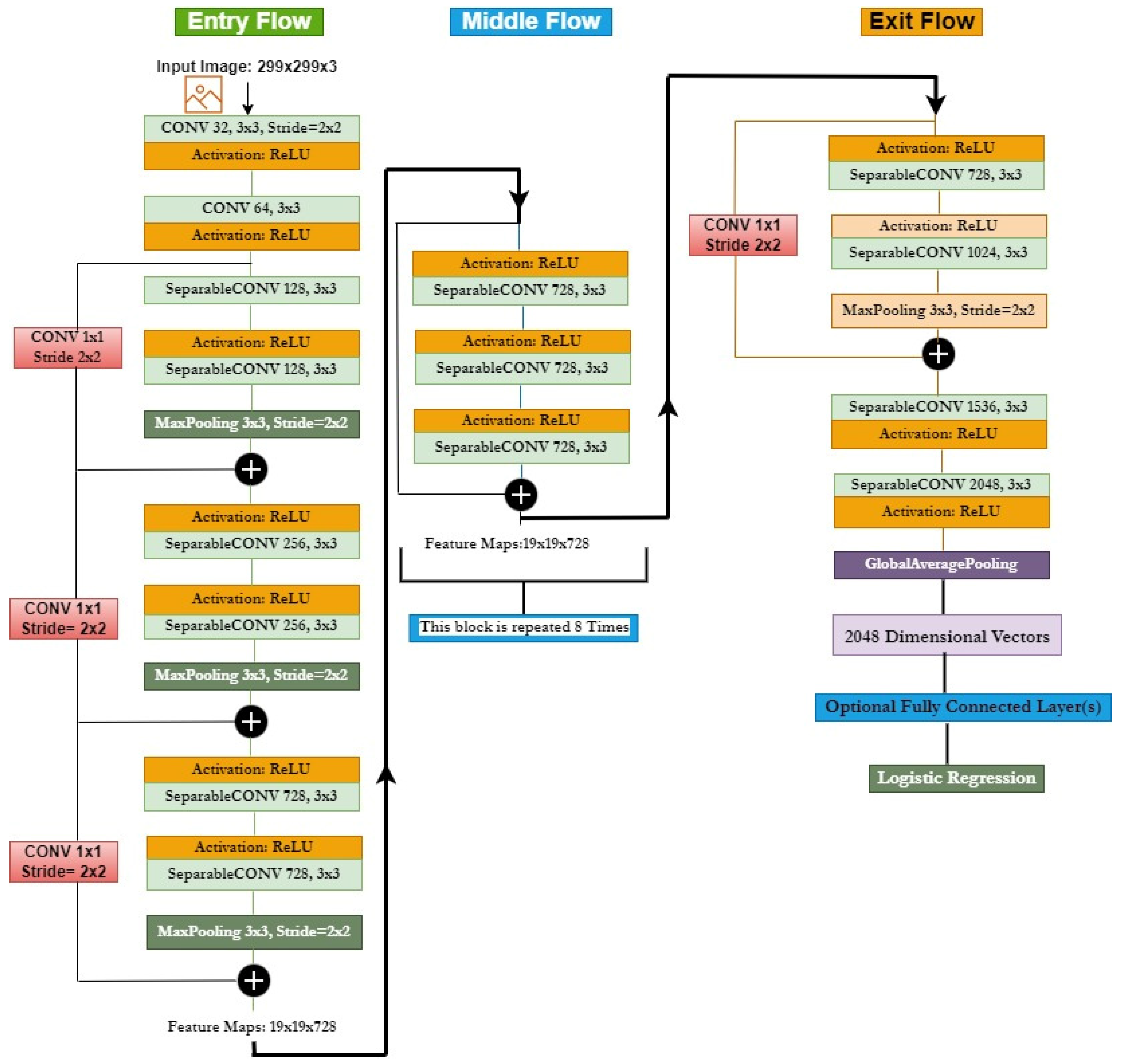
We have used well-established CNN architectures to extract optimized features from the images, called the Xception model. It was developed by Google researchers and is an extreme version of the Google Inception model, which has obtained excellent classification performance as compared to VGGNet, ResNet and Inception model for the image classification task. The Xception model replaces the Inception model with depth-wise separable convolutions instead of inception modules. It is 71 layers deep and trained on the ImageNet database with more than a million images. As shown in Figure 3, the network architecture consists of a linear stack with depth-wise separable convolution layers and residual connections.
The input data first go through the entry flow block, followed by the middle flow, which is repeated eight times, and, at last, through the exit flow block. Here, all the convolution and separable convolution layers are followed by batch normalization. To extract features from this pretrained Xception CNN model, fine-tuning of this model is conducted using ISIC skin lesion images to obtain higher quality features from the images.
We have removed the last FC layer of the Xception model and replaced it with three new layers, which are the dropout layer to prevent the model from overfitting, the global average pooling layer to reduce the total number of parameters in the model to minimize overfitting and the dense or FC layer with two nodes to solve the binary classification problem, as shown in Figure 4.
The model is initialized with ImageNet weights on which it is pretrained, and the weights are updated during the fine-tuning of all the layers during the training of our proposed model on the ISIC skin lesion dataset so that the pretrained Xception model integrates well into our new CNN model.
In this proposed model, we have used different optimizers during the fine-tuning of the model. The optimizers utilized in our experiments are Adam [27], an adaptive learning rate optimizer; Adamax based on Adam, an adaptive learning rate optimizer; LazyAdam for handling sparse updates, another variant of the Adam optimizer [28]; Nadam, which is again a variant of Adam with nesterov momentum [29]; RMSProp, i.e., root mean square propagation [30]; SGD, i.e., stochastic gradient descent [31].
In machine learning, optimization is the task of minimizing the loss function (), where w is the model’s parameter, ∈ Rd. It is conducted by updating the parameters in the direction opposite to the gradient of the objective function ∇w() with respect to the model’s parameters. The step size we take to reach a local minimum is called the learning rate and is represented by η.
In the case of SGD, it performs a parameter update for each of the training images x(i) and its corresponding label y(i) with the following equation:
Momentum can be added to SGD to accelerate it in the relevant direction. It adds a fraction γ of the past time update vector vt−1 to the current update vector vt as:
In this work, we used SGD with nesterov acceleration, which can significantly speed up the training process and improve the convergence. Nesterov acceleration is added to the above equation to give momentum a slowdown phase when slopes come up again. The momentum term γvt−1 is used here to move the parameters , and by calculating w − γvt−1, we obtain an approximation of the next position of the model’s parameters. The gradient is now calculated with respect to the future position of the model’s parameters:
Exponentially decaying average of past gradients, just like momentum, is kept by the Adam optimizer. Momentum can be visualized as a ball running down a slope, but Adam can be pictured as a heavy ball with friction, preferring flat minima on the error surface [27]. The decaying averages in Adam for past and past squared gradients, and , are calculated as follows:
where the first moment and the second momentum of the gradients are and , respectively, and are decay rates and is the gradient on the current mini-batch. The biased correction equation for Adam is:
Finally, to perform the weight update, the following equation is used:
where the default values of β1 and β2 are 0.9 and 0.999 and 10−8 for ϵ.
Adamax, which is based on the infinity norm, is also used as a variant of the Adam optimizer. It is used for sparse parameter updates and has the following set of equations for optimization:
The LazyAdam optimizer handles the updates, which are sparse, more efficiently. For each trainable variable, Adam maintains two moving-average accumulators, which are updated at every step. LazyAdam handles the updates of a gradient in a lazy manner for sparse variables. Instead of updating accumulators for all indices, it only updates accumulators for sparse variable indices that only appear in the current batch. Comparing it with the Adam optimizer can provide the best performance model training in some of the applications [28].
Further, the RMSProp [30] optimizer is used, which is used to resolve the radically diminishing learning rates. It is similar to the SGD algorithm with momentum, but the oscillations are restricted in the vertical direction here. The loss function in RMSProp is minimized based on the following:
where is:
is the value of the momentum or decay rate, which is a hyperparameter and is generally set to value of 0.9, and is used to prevent divide by zero error.
The Nadam optimizer used is very much similar to the Adam optimizer. Like Adam with nesterov momentum [29], we have discussed above in SGD or RMSProp with momentum term. The update rule in Nadam is as follows:
where is the current momentum vector for bias correction.
We used the sparse categorical cross-entropy loss function, which calculates the cross-entropy loss between the labels and predictions with every optimizer algorithm we utilized. Sparse categorical cross-entropy loss is like the categorical cross-entropy loss function defined in Equation (18) below. The only difference between them is related the truth labels definition. In sparse categorical cross-entropy, the truth labels are encoded in the form of an integer such as [1,2] for 2-class problems, while in categorical cross-entropy, it is [1, 0], [0, 1] for 2-class problems.
where n is the number of classes, is the truth label and is the softmax classifier probability for ith class.
In our experiments, the initial learning rate is set to 0.0001 and the batch size to 32 for all the optimizers we have used. The number of epochs is set to 64 for all the optimizers, except for SGD, for which we have set it to 128. The momentum term for SGDM is set to 0.0, and , and are set to 0.9, 0.999 and 0.0000001, respectively, in Adam, Nadam, Adamax and LazyAdam. In RMSProp, the values of , momentum and are set to 0.9, 0 and 0.0000001, respectively.
Early stopping criteria are used during training to stop the process when the validation accuracy has stopped improving. It is a form of regularization that is used to avoid overfitting [32]. The following parameters are set for this:
This is designed to stop the training process if the validation accuracy metric does not improve after 5 epochs. Here, the model’s weight will also be restored from the epoch that has the best value of the monitored quantity as per the following expression:
The dropout value is set to 0.50, which means 50 percent of randomly selected neurons are dropped out or ignored during training. It means on the forward pass, the contribution of these neurons in the activation of downstream neurons is temporally removed, and no weight updates are applied to the neurons on the backward pass [33]. This technique helps deal with overfitting during the training process.
Finally, the activation function used in the last fully connected layer is the softmax activation function. Our model is configured to output 2 values, i.e., malignant or benign. Hence, the softmax function normalizes the output values by converting them from weighted sum values into probabilities that sum to one [34].
3. Experimental Setup and Results
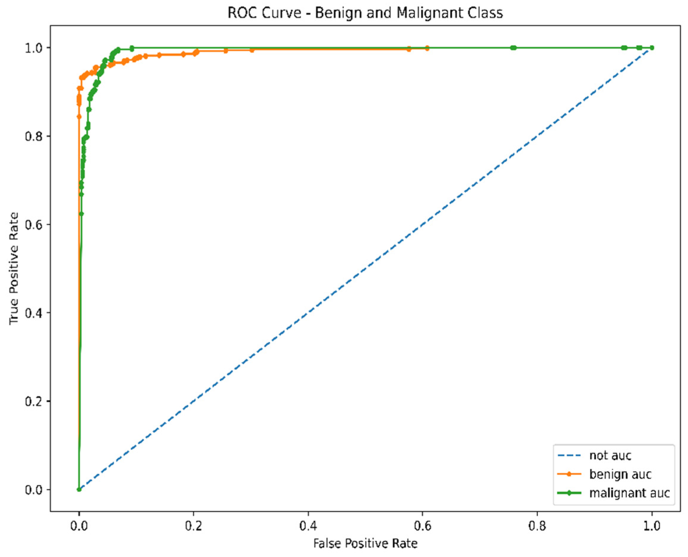
The model is implemented in Google Colabs, a cloud facility provided by Google to implement machine learning algorithms. Colabs provide very powerful processing units such as GPU and TPU. The proposed model is implemented on Tesla P100-PCIE-16GB GPU using Python programming language. After training and validating the proposed CNN model on the augmented dataset, the model was tested on 1000 unlabeled images of melanoma and benign. This section discusses training, validation, and testing processes and the model’s performance analysis during these phases using metrics such as training accuracy, training loss, validation accuracy, validation loss, prediction accuracy and prediction loss. AUC, which stands for area under curve, determines whether the model is capable of distinguishing between classes and is also calculated for the proposed model. The higher the AUC value, the better the model is at predicting benign as benign and malignant as malignant.
3.1. Training and Validation Process
During the training and validation process, while loading the Xception model, the “include_top” argument is set to False to remove the fully-connected output layer of the Xception model, allowing layers to be added for the proposed model by using Xception as a base model. The Xception model is loaded with weights = “imagenet”, as it is trained on the imagenet dataset, which has millions of training images in 1000 categories. Because of this, the Xception model will have prior knowledge about basic shapes, and then, layers added on top of this knowledge for the proposed model are kept trainable so that it can adjust to the skin lesion dataset. The initial learning rate is set to 0.0001, the batch size is set to 32 and drop out is set to 0.50. The number of epochs are set to 64 for Adam, Adamax, LazyAdam, Nadam and RMSProp, and for SGD, it is set to 128. The activation function used in the dense layer is the softmax activation function. All the hyperparameters discussed here are the same for each experiment using different optimizers, except for the number of epochs, which is more for SGD. The training and validation process is executed side by side the classical approach using 67: 33 split of training data into training and validation set, respectively. Table 1 shows the training performance of the model utilizing different optimizers.
From the above results, the best training accuracy of the model is achieved using the LazyAdam optimizer and the lowest training loss using Adam optimizer. Additionally, the validation loss is lowest using LazyAdam, and validation accuracy is highest using RMSProp optimizer. By including early stopping criteria, the model reached the best performance in epoch 7 using Nadam and LazyAdam, while it goes up to 66 epochs using the SGD optimizer. In terms of training and validation time, the model took the least time using the Nadam optimizer, and it took the longest time using the SGD optimizer. The reason for a longer time in SGD can be poor handling of heavy-tailed noise, whereas Nadam performs gradient clipping coordinate-wise in an implicit manner to tackle heavy-tailed noise. Therefore, this clipping makes Nadam significantly faster than SGD.
3.2. Testing Process
After the training performance, the classification performance of the model is discussed. The various classification metrics were calculated for the model, such as sparse categorical cross-entropy loss, accuracy for predicting image correctly as benign or malignant, average accuracy, average precision, average recall, average specificity, average sensitivity and average value of area under the curve. These metrics were calculated using different optimizers in this proposed work. Table 2 shows the classification performance of the proposed model utilizing other optimizers. Various metrics are used here to analyze the model performance for predicting the image class, such as accuracy, sensitivity, specificity and precision. The accuracy is an essential measure in medical image analysis as it gives the ratio between the samples that are correctly classified and the total number of samples in the test dataset. The sensitivity or recall or True Positive Rate (TPR) is also considered an essential metric in medical image analysis, as the goal is to miss as few positive samples as possible to obtain a high recall or sensitivity value. It is the rate of correctly classified positive samples and is calculated as the ratio between positive samples correctly classified and the entire dataset assigned to the positive class.
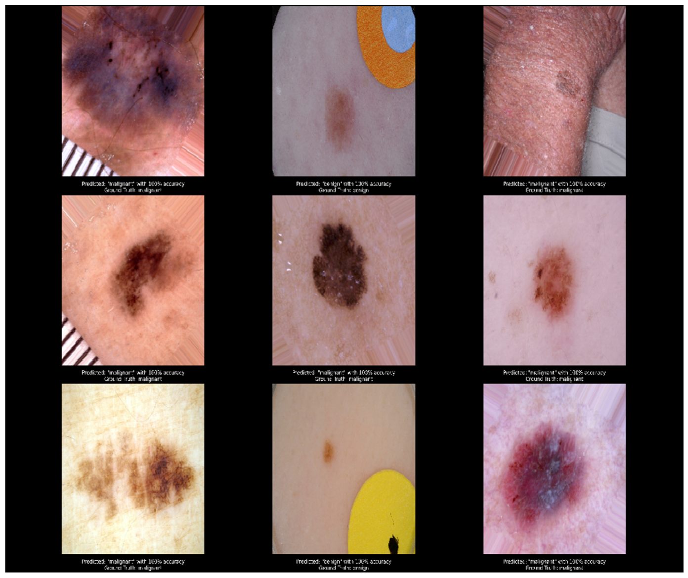
The specificity is negative or opposite of the sensitivity, denoting the rate of correctly classified negative samples. It is calculated as the ratio between negative samples that are correctly classified and all samples that are classified as negative. Finally, precision denotes the proportion of relevant retrieved samples, and it is calculated as the ratio between samples that are correctly classified and all samples assigned to that class. The model loss is very low using the Adamax optimizer, while the class-wise accuracy and average accuracy are highest with the RMSProp optimizer. The average precision, specificity and sensitivity values are also highest using the RMSProp optimizer. In contrast, the average value of area under the curve is highest using the Adamax optimizer, which means that the model performs best at predicting benign as benign and malignant as malignant using the Adamax optimizer.
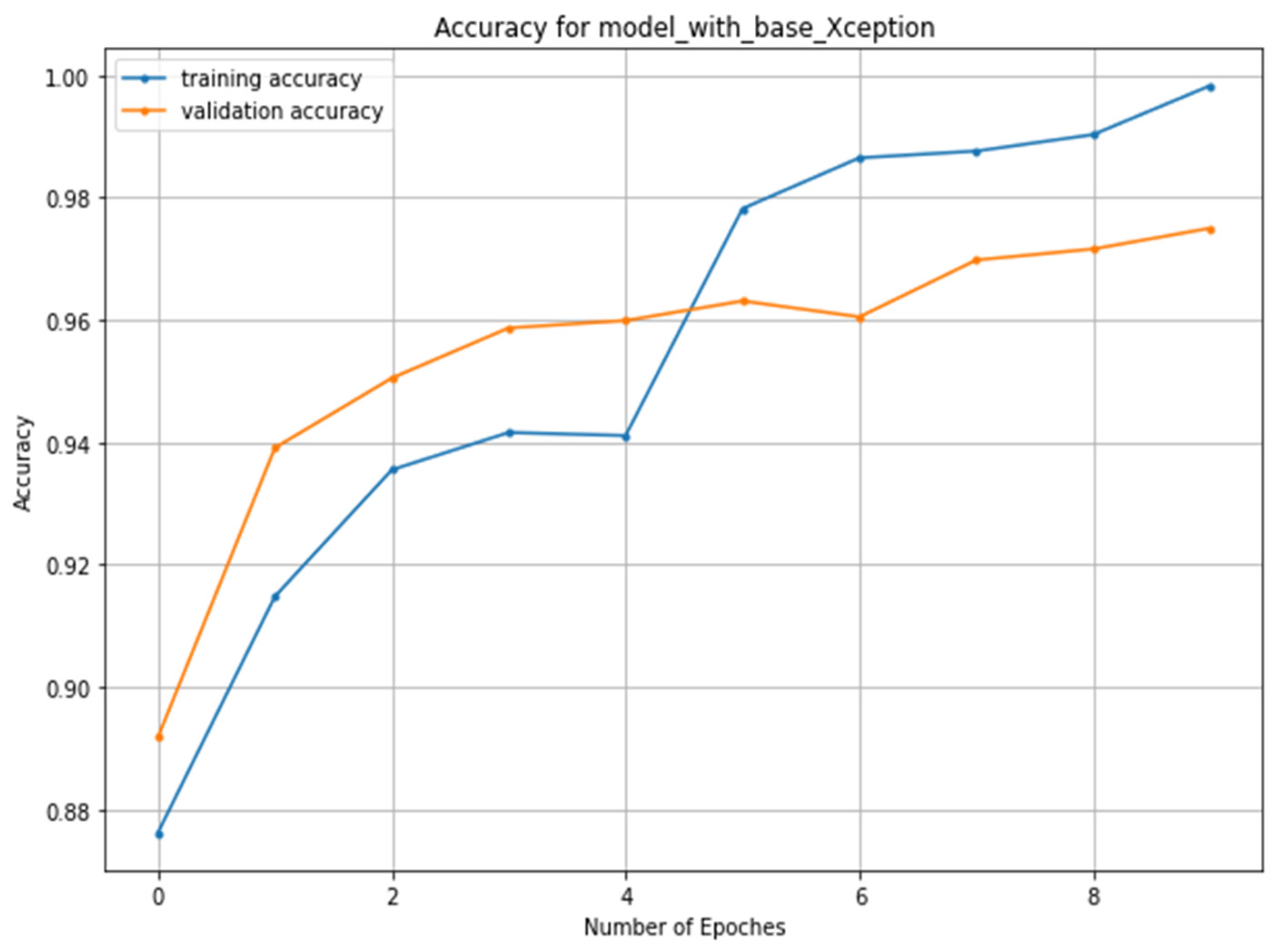
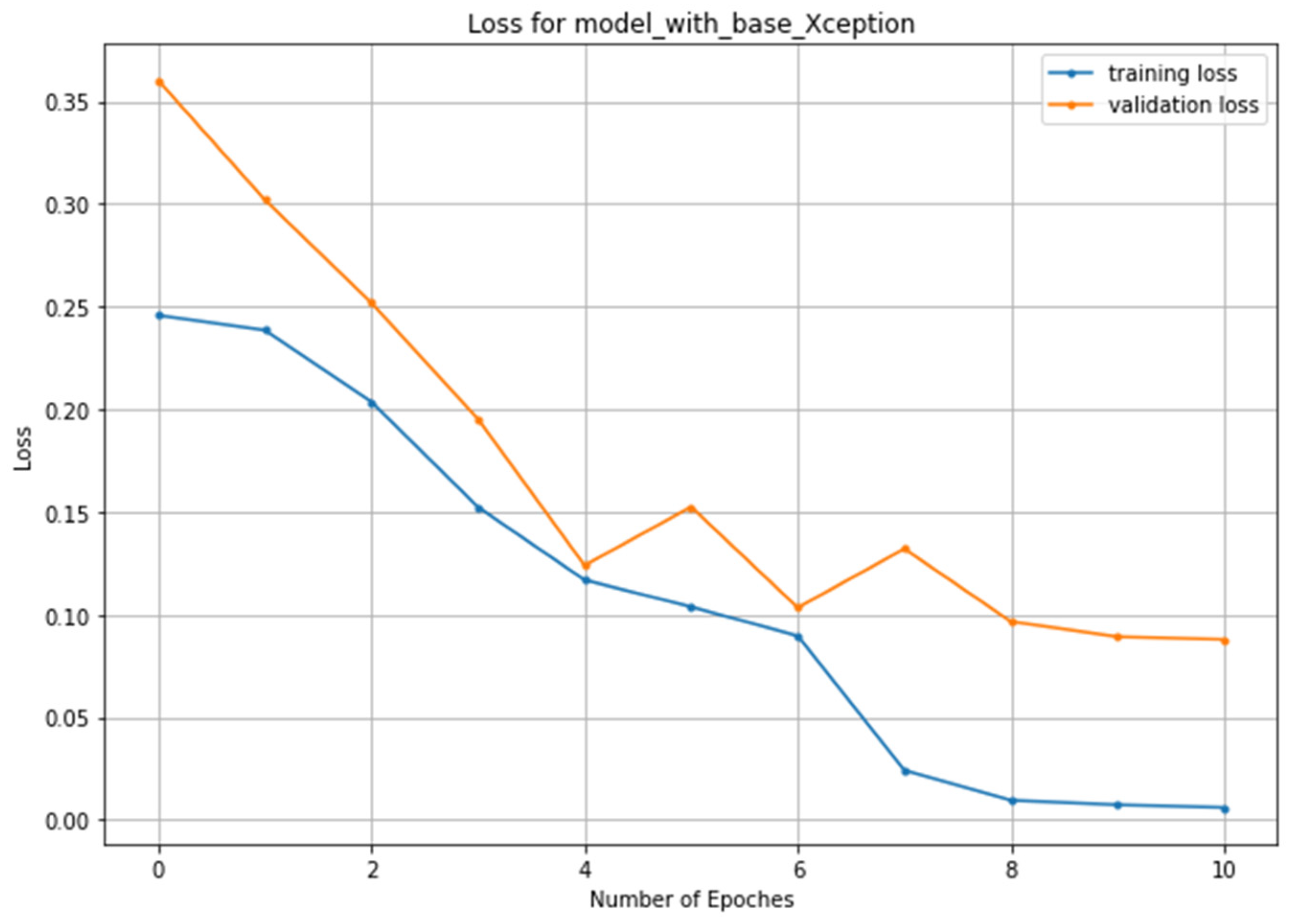
The graphs for training accuracy, validation accuracy, training loss and validation loss with the best values using different optimizers are shown in Figure 5 and Figure 6, respectively. For the classification performance, the predicted results versus ground truth values for the RMSProp optimizer are shown in Figure 7, and ROC–AUC curves are also plotted using the RMSProp optimizer in Figure 8.
Now to prove that the proposed model is the best compared to other state-of-the-art models developed so far that have used the same dataset as used in this work, a comparison is presented below in Table 3.
The above results proved that the proposed model achieved the best figures for accuracy, AUC, sensitivity and specificity compared to other models. The proposed model also achieved the highest training accuracy of 99.83%, which is the best among all the works conducted for skin lesion classification problems.
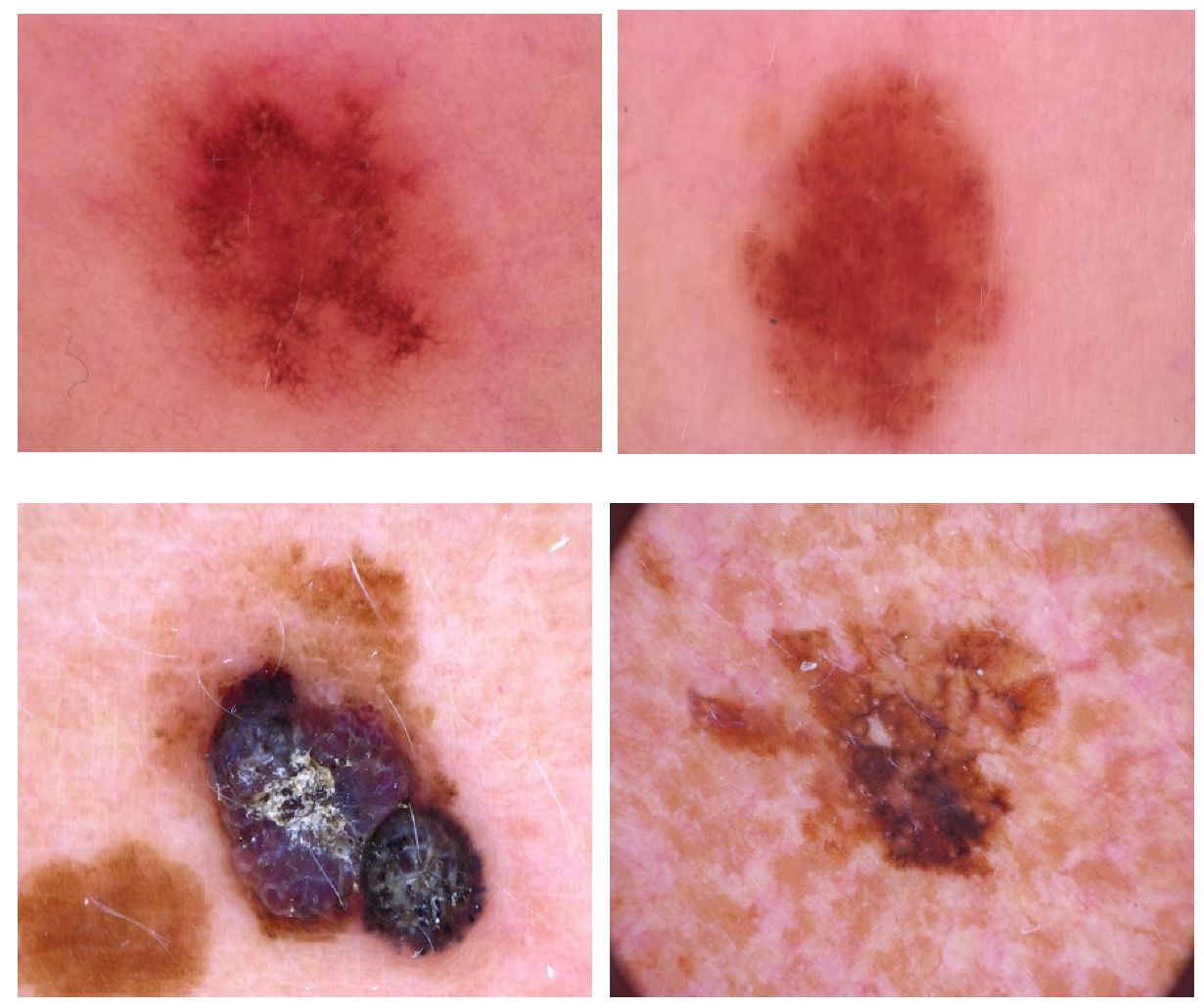
To further check the generalizability of the proposed model, it is trained and tested again on the HAM10000 [39] dataset, which stands for “Human Against Machine”. It consists of dermatoscopic images collected, acquired and stored from different populations and different modalities. A total of 10,015 images of melanocytic nevi, melanoma and others are included in this dataset. We have extracted nevi and melanoma images from this dataset only to show the binary classification as conducted on the ISIC dataset. The sample images of these classes is shown in the Figure 9 below.
The dataset has 7037 images for both classes mentioned, out of which 33% of data is taken for validation and the remaining for training purposes, while the test dataset consists of 781 images of both classes. All the preprocessing steps are the same as the ISIC dataset, including data augmentation of the training set. The model hyperparameters are also the same, and the optimizer utilized is RMSProp, as it has given the best results on the ISIC dataset. Table 4 below shows the model’s performance on the HAM10000 dataset during training and testing compared to other state-of-the-art models on the same dataset.
Table 4 above shows that the proposed model has outperformed other models trained and tested on the HAM10000 dataset in terms of testing and classification accuracy. Thus, the generalizability of the model is proved for diverse datasets. The proposed model can be applied to different datasets due to its better performance.
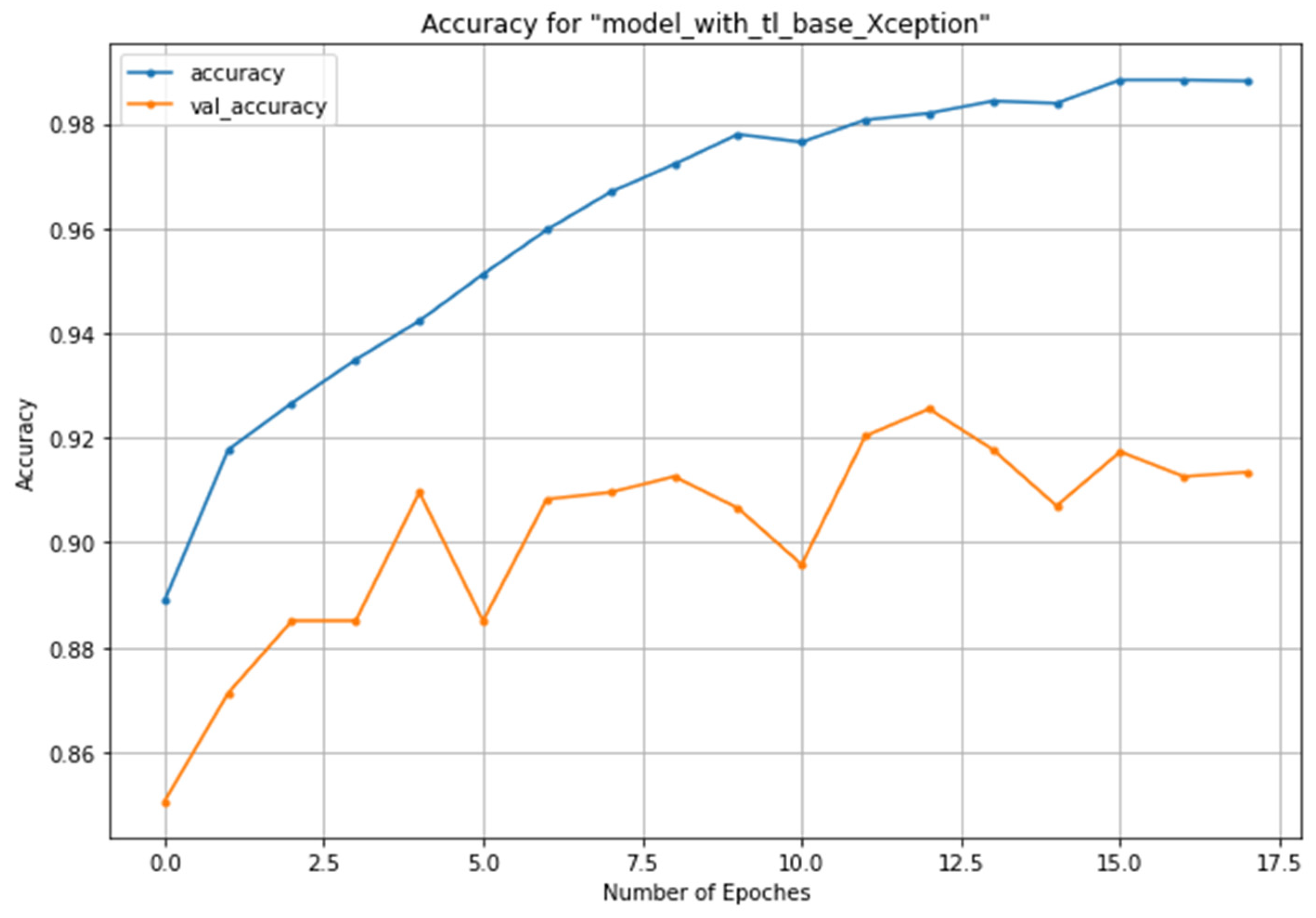
The training vs. validation accuracy plot of the proposed model on the HAM10000 dataset is shown in Figure 10 below, where the validation accuracy is 0.9134, which shows the model does not overfit the training data.
4. Discussion
The main contribution of this work is proposing a CNN architecture based on a transfer learning approach for melanoma skin cancer classification. By utilizing the Xception model pre-trained on the ImageNet dataset and fine-tuning it with different types of optimizers and hyperparameter settings, the proposed model gives very promising results without the need for extensive preprocessing of the input skin lesion images, and there is no need for image segmentation, which most of the previous researchers used in their work for segmenting the lesion area. To justify using early stopping criteria, Table 1 clearly shows the whole epoch reached during training by the model for each optimizer. The training time and system resources are saved using this technique. Additionally, restoring the models’ weights to the best-valued epoch further reduces the chances of degradation in classification results.
Moreover, comparing the results using different optimizers shows that models have excellent performances in almost all cases but are slightly higher in the case of RMSProp and LazyAdam optimizers considering loss and accuracy during training, validation and classification. Further, Table 3 shows that the accuracy, specificity and sensitivity are best for the proposed model compared to other state-of-the-art models. The model also achieved the best results when trained and tested on the HAM10000 dataset as compared to other methods. Therefore, it can be accepted as a generalized model for different types of datasets.
As far as the proposed model’s real-time applicability analysis is concerned, a user-friendly mobile application can be designed to identify melanoma. The user will be able to click the picture or upload a picture with melanoma on the device. The image will be sent to the server where the proposed model is implemented. The feature parameters of the image will be calculated, and the trained model can carry out image classification. The entire process can be completed in few seconds as we have seen the classification time of the proposed model is 2 s. Thus, with the help of a mobile application, it will be very easy to identify melanoma during the early stages and make the task of dermatologists easier.
5. Conclusions and Future Work
Melanoma detection using deep learning architectures gives very promising results, but the lack of large datasets to train the CNN model makes delivering good classification performance challenging. In this paper, we have proposed a transfer learning-based CNN model and data augmentation techniques applied to raise training and classification accuracy. Additionally, various optimizers are tested on the proposed model to obtain the best results to be further applied to different datasets, as conducted in this work on the HAM10000 dataset. The main motive of this work is to obtain a generalized model to classify skin lesion images into different classes and on different types of datasets.
The augmented images distribution is different from the original images, so it can lead to data bias, affecting the model’s performance. In the future, generative adversarial networks (GANs), which use a novel method for data augmentation, can generate a large amount of synthetic data from the original one. We used the CNN model based on the transfer learning approach for melanoma and benign classification and obtained promising results. Still, as part of future research, a CNN model can be developed and trained from scratch using the large amount of data generated through GAN. Thus, the model can be utilized using a transfer learning approach for other forms of medical image classification by fine-tuning it if the dataset for the problem is minimal.
Author Contributions
Conceptualization, M.N.Q. and M.S.U.; Methodology, M.N.Q.; software, M.N.Q.; validation, M.N.Q., M.S.U. and S.S.; formal analysis, M.N.Q. and S.S.; investigation, M.N.Q. and M.S.U.; resources, M.N.Q.; data curation, M.N.Q.; writing—original draft preparation, M.N.Q.; writing—review and editing, M.N.Q., M.S.U. and S.S.; visualization, M.N.Q.; supervision, M.S.U.; funding acquisition, S.S. All authors have read and agreed to the published version of the manuscript.
Funding
This research was supported by the Princess Nourah bint Abdulrahman University Researchers Supporting Project number (PNURSP2022R259), Princess Nourah bint Abdulrahman University, Riyadh, Saudi Arabia.
Institutional Review Board Statement
Not applicable.
Informed Consent Statement
Not applicable.
Data Availability Statement
The data are publicly available at https://www.isic.org/ (accessed on 20 November 2021) and https://dataverse.harvard.edu/dataset.xhtml?persistentId=doi:10.7910/DVN/DBW86T (accessed on 12 March 2022).
Acknowledgments
This research was supported by the Princess Nourah bint Abdulrahman University, Riyadh, Saudi Arabia. All of the authors are very thankful to the funding agency.
Conflicts of Interest
The authors declare no conflict of interest.
Abbreviations
| CNN | Convolution Neural Network |
| ISIC | International Skin Image Collaboration |
| BRAF | Human Gene That Encodes a Protein Called B-Raf |
| VGG | Visual Geometry Group |
| ResNet | Residual Network |
| Adam | Adaptive Moment Estimation |
| Nadam | Nesterov-Accelerated Adaptive Moment Estimation |
| SGD | Stochastic Gradient Descent |
| RMSProp | Root Mean Square Propagation |
| GPU | Graphics Processing Unit |
| TPU | Tensor Processing Unit |
| ROC | Receiver Operating Characteristic Curve |
| AUC | Area Under ROC Curve |
References
- American Cancer Society: Melanoma Skin Cancer. Available online: https://www.cancer.org/cancer/melanoma-skin-cancer/ (accessed on 9 April 2022).
- Goncharova, Y.; Attia, E.A.; Souid, K.; Vasilenko, I.V. Dermoscopic features of facial pigmented skin lesions. ISRN Dermatol. 2013, 2013, 546813. [Google Scholar] [CrossRef]
- Zalaudek, I.; Lallas, A.; Moscarella, E.; Longo, C.; Soyer, H.P.; Argenziano, G. The dermatologist’s stethoscope-traditional and new applications of dermoscopy. Dermatol. Pract. Concept. 2013, 3, 67–71. [Google Scholar] [CrossRef] [PubMed] [Green Version]
- Argenziano, G.; Soyer, H.P. Dermoscopy of pigmented skin lesions—A valuable tool for early diagnosis of melanoma. Lancet Oncol. 2001, 2, 443–449. [Google Scholar] [CrossRef]
- Siegel, R.L.; Miller, K.D.; Jemal, A. Cancer statistics, 2018. CA Cancer J. Clin. 2018, 68, 7–30. [Google Scholar] [CrossRef]
- Gola Isasi, A.; García Zapirain, B.; Méndez Zorrilla, A. Melanomas non-invasive diagnosis application based on the ABCD rule and pattern recognition image processing algorithms. Comput. Biol. Med. 2011, 41, 742–755. [Google Scholar] [CrossRef] [PubMed]
- Haenssle, H.A.; Fink, C.; Schneiderbauer, R.; Toberer, F.; Buhl, T.; Blum, A.; Kalloo, A.; Hassen, A.B.H.; Thomas, L.; Enk, A.; et al. Man against machine: Diagnostic performance of a deep learning convolutional neural network for dermoscopic melanoma recognition in comparison to 58 dermatologists. Ann. Oncol. 2018, 29, 1836–1842. [Google Scholar] [CrossRef] [PubMed]
- Szegedy, C.; Liu, W.; Jia, Y.; Sermanet, P.; Reed, S.; Anguelov, D.; Erhan, D.; Vanhoucke, V.; Rabinovich, A. Going deeper with convolutions. In Proceedings of the 2015 IEEE Conference on Computer Vision and Pattern Recognition (CVPR), Boston, MA, USA, 7–12 June 2015. [Google Scholar]
- Krizhevsky, A.; Sutskever, I.; Hinton, G.E. ImageNet classification with deep convolutional neural networks. In Proceedings of the 25th International Conference on Neural Information Processing Systems—Volume 1 (NIPS’12), Red Hook, NY, USA, 3–6 December 2012; pp. 1097–1105. [Google Scholar]
- He, K.; Zhang, X.; Ren, S.; Sun, J. Deep residual learning for image recognition. In Proceedings of the 2016 IEEE Conference on Computer Vision and Pattern Recognition (CVPR), Las Vegas, NV, USA, 27–30 June 2016. [Google Scholar]
- Simonyan, K.; Zisserman, A. Very Deep Convolutional Networks for Large-Scale Image Recognition. In Proceedings of the 3rd International Conference on Learning Representations (ICLR2015), San Diego, CA, USA, 7–9 May 2015; Available online: https://arxiv.org/abs/1409.1556 (accessed on 10 November 2021).
- Deng, J.; Dong, W.; Socher, R.; Li, L.J.; Li, K.; Fei-Fei, L. ImageNet: A large-scale hierarchical image database. In Proceedings of the 2009 IEEE Conference on Computer Vision and Pattern Recognition (CVPR), Miami, FL, USA, 20–25 June 2009. [Google Scholar]
- Vasconcelos, C.; Vasconcelos, B.N. Increasing Deep Learning Melanoma Classification by Classical and Expert Knowledge Based Image Transforms. arXiv 2017, arXiv:abs/1702.07025. [Google Scholar]
- Lopez, A.R.; Giro-i Nieto, X.; Burdick, J.; Marques, O. Skin lesion classification from dermoscopic images using deep learning techniques. In Proceedings of the 13th IASTED International Conference on Biomedical Engineering (BioMed), Innsbruck, Austria, 20–21 February 2017. [Google Scholar]
- Tajbakhsh, N.; Shin, J.Y.; Gurudu, S.R.; Hurst, R.T.; Kendall, C.B.; Gotway, M.B.; Liang, J. Convolutional Neural Networks for Medical Image Analysis: Full Training or Fine Tuning? IEEE Trans. Med. Imaging 2016, 35, 1299–1312. [Google Scholar] [CrossRef] [PubMed] [Green Version]
- Kawahara, J.; BenTaieb, A.; Hamarneh, G. Deep features to classify skin lesions. In Proceedings of the 13th International Symposium on Biomedical Imaging, (IEEE), Prague, Czech Republic, 16 June 2016; pp. 1397–1400. [Google Scholar] [CrossRef]
- Codella, N.; Cai, J.; Abedini, M.; Garnavi, R.; Halpern, A.; Smith, J.R. Deep learning, sparse coding, and SVM for melanoma recognition in dermoscopy images. In Proceedings of the 6th International Workshop on Machine Learning in Medical Imaging, Held in Conjunction with MICCAI 2015, Munich, Germany, 5 October 2015; pp. 118–126. [Google Scholar]
- DeVries, T.; Ramachandram, D. Skin Lesion Classification Using Deep Multi-scale Convolutional Neural Networks. arXiv 2017, arXiv:1703.01402. [Google Scholar] [CrossRef]
- Szegedy, C.; Ioffe, S.; Vanhoucke, V.; Alemi, A. Inception-v4, Inception-ResNet and the Impact of Residual Connections on Learning. In Proceedings of the AAAI Conference on Artificial Intelligence, Stanford, CA, USA, 21–23 March 2016. [Google Scholar]
- Sabbaghi, S.; Aldeen, M.; Garnavi, R. A deep bag-of-features model for the classification of melanomas in dermoscopy images, 2016. In Proceedings of the 38th Annual International Conference of the IEEE Engineering in Medicine and Biology Society (EMBC), Orlando, FL, USA, 16–20 August 2016; pp. 1369–1372. [Google Scholar] [CrossRef]
- Deivanayagampillai, N.; Suruliandi, A.; Kavitha, J. Melanoma Detection in Dermoscopic Images using Global and Local Feature Extraction. Int. J. Multimed. Ubiquitous Eng. 2017, 12, 19–27. [Google Scholar] [CrossRef]
- Nasiri, S.; Helsper, J.; Jung, M.; Fathi, M. DePicT Melanoma Deep-CLASS: A deep convolutional neural networks approach to classify skin lesion images. BMC Bioinform. 2020, 21 (Suppl. 2), 84. [Google Scholar] [CrossRef] [Green Version]
- Chollet, F. Xception: Deep Learning with Depth Wise Separable Convolutions. In Proceedings of the 2017 IEEE Conference on Computer Vision and Pattern Recognition (CVPR), Honolulu, HI, USA, 21–26 July 2017; pp. 1800–1807. [Google Scholar]
- The International Skin Imaging Collaboration (ISIC). Available online: https://www.isic-archive.com/#!/topWithHeader/onlyHeaderTop/gallery (accessed on 20 November 2021).
- Mikołajczyk, A.; Grochowski, M. Data augmentation for improving deep learning in image classification problem. In Proceedings of the 2018 International Interdisciplinary PhD Workshop (IIPhDW), Świnouście, Poland, 9–12 May 2018; pp. 117–122. [Google Scholar]
- Gu, S.; Pednekar, M.; Slater, R. Improve Image Classification Using Data Augmentation and Neural Networks. SMU Data Sci. Rev. 2019, 2, 1. [Google Scholar]
- Kingma, D.; Ba, J. Adam: A Method for Stochastic Optimization. In Proceedings of the 3rd International Conference on Learning Representations, San Diego, CA, USA, 7–9 May 2015. [Google Scholar]
- LazyAdam a Variant of Adam Optimizer. Available online: https://tensorflow.org/addons/api_docs/python/tfa//optimizers//La-zyAdam (accessed on 18 December 2021).
- Dozat, T. Incorporating Nesterov Momentum into Adam. In Proceedings of the ICLR Workshop, San Juan, Puerto Rico, 2–4 May 2016. [Google Scholar]
- Tieleman, T.; Hinton, G. Lecture 6.5-rmsprop: Divide the gradient by a running average of its recent magnitude. Coursera Neural Netw. Mach. Learn. 2012, 4, 26–31. [Google Scholar]
- Robbins, H.; Monro, S. A stochastic approximation method. Ann. Math. Stat. 1951, 22, 400–407. [Google Scholar] [CrossRef]
- Prechelt, L. Early Stopping—But When? In Neural Networks: Tricks of the Trade; Montavon, G., Orr, G.B., Müller, K.R., Eds.; Lecture Notes in Computer Science; Springer: Berlin, Heidelberg, 2012; Volume 7700. [Google Scholar] [CrossRef]
- Srivastava, N.; Hinton, G.E.; Krizhevsky, A.; Sutskever, I.; Salakhutdinov, R. Dropout: A simple way to prevent neural networks from overfitting. J. Mach. Learn. Res. 2014, 15, 1929–1958. [Google Scholar]
- Nwankpa, C.; Ijomah, W.; Gachagan, A.; Marshall, S. Activation Functions: Comparison of trends in Practice and Research for Deep Learning. In Proceedings of the 2nd International Conference on Computational Sciences and Technology, Jamshoro, Pakistan, 17–19 December 2020. [Google Scholar]
- Harangi, B. Skin lesion classification with ensembles of deep convolutional neural networks. J. Biomed. Inform. 2018, 86, 25–32. [Google Scholar] [CrossRef] [PubMed]
- Yu, L.; Chen, H.; Dou, Q.; Qin, J.; Heng, P.A. Automated Melanoma Recognition in Dermoscopy Images via Very Deep Residual Networks. IEEE Trans. Med. Imaging 2017, 36, 994–1004. [Google Scholar] [CrossRef] [PubMed]
- Albahar, M.A. Skin Lesion Classification Using Convolutional Neural Network with Novel Regularizer. IEEE Access 2019, 7, 38306–38313. [Google Scholar] [CrossRef]
- Yoshida, T.; Celebi, M.E.; Schaefer, G.; Iyatomi, H. Simple and effective preprocessing for automated melanoma discrimination based on cytological findings. In Proceedings of the IEEE International Conference on Big Data, Washington, DC, USA, 5–8 December 2016. [Google Scholar]
- Tschandl, P.; Rosendahl, C.; Kittler, H. The HAM10000 dataset, a large collection of multi-sources dermatoscopic images of common pigmented skin lesions. Sci. Data 2018, 5, 180161. [Google Scholar] [CrossRef] [PubMed]
- Ali, S.; Sipon Miah, J.H.; Rahman, M.; Islam, K. An enhanced technique of skin cancer classification using deep convolutional neural network with transfer learning models. Mach. Learn. Appl. 2021, 5, 100036. [Google Scholar] [CrossRef]
- Sinha, D.; El-Sharkawy, M. Thin MobileNet: An Enhanced MobileNet Architecture. In Proceedings of the IEEE 10th Annual Ubiquitous Computing, Electronics & Mobile Communication Conference (UEMCON), New York, NY, USA, 10–12 October 2019; pp. 280–285. [Google Scholar] [CrossRef]
- Carcagnì, P.; Leo, M.; Cuna, A.; Mazzeo, P.L.; Spagnolo, P.; Celeste, G.; Distante, C. Classification of skin lesions by combining multilevel learnings in a densenet architecture. In Proceedings of the International Conference on Image Analysis and Processing, Trento, Italy, 9–13 September 2019; pp. 335–344. [Google Scholar] [CrossRef]
- Ameri, A. A Deep Learning Approach to Skin Cancer Detection in Dermoscopy Images. J. Biomed. Phys. Eng. 2020, 10, 801–806. [Google Scholar] [CrossRef]
- Pham, T.C.; Tran, G.S.; Nghiem, T.P.; Doucet, A.; Luong, C.M.; Hoang, V. A Comparative Study for Classification of Skin Cancer. In Proceedings of the International Conference on System Science and Engineering (ICSSE), Dong Hoi City, Vietnam, 19–21 July 2019. [Google Scholar] [CrossRef]
- Nugroho, A.; Slamet, I.; Sugiyanto. Skins cancer identification system of HAMl0000 skin cancer dataset using convolutional neural network. In Proceedings of the AIP Conference, Surakata, Indonesia, 19 July 2019; Volume 2202, p. 020039. [Google Scholar] [CrossRef]
Figure 1.
Proposed Methodology.

Figure 2.
Sample images from the ISIC archive dataset: benign (row 1) and melanoma (row 2).

Figure 3.
Xception model network architecture [23].
Figure 3.
Xception model network architecture [23].

Figure 4.
Proposed CNN model based on pretrained Xception architecture.

Figure 5.
Training and validation accuracy using the LazyAdam optimizer.

Figure 6.
Training and validation loss using the Adam optimizer.

Figure 7.
Ground truth vs. predicted value using the RMSProp optimizer: column 1 and 3 shows malignant predicted with 100% accuracy; column 2 top and bottom images are of benign tumors predicted with 100% accuracy.
Figure 7.
Ground truth vs. predicted value using the RMSProp optimizer: column 1 and 3 shows malignant predicted with 100% accuracy; column 2 top and bottom images are of benign tumors predicted with 100% accuracy.

Figure 8.
ROC–AUC curve using the RMSProp optimizer.

Figure 9.
Sample images from the HAM10000 dataset: nevi (row 1) and melanoma (row 2).

Figure 10.
Training and validation accuracy using the HAM1000 dataset.


Table 1.
Performance of the proposed CNN model during training.
| Optimizer | Training Loss | Training Accuracy | Validation Loss | Validation Accuracy | Total Epochs Reached | Training Time (in Seconds) |
|---|---|---|---|---|---|---|
| SGD | 0.2423 | 93.33% | 0.2059 | 95.38% | 66 | 9738.66 |
| Adam | 0.0060 | 99.78% | 0.0879 | 97.64% | 11 | 2170.34 |
| Adamax | 0.0478 | 98.25% | 0.0982 | 95.85% | 9 | 1345.32 |
| Nadam | 0.0364 | 98.59% | 0.1181 | 96.39% | 7 | 1092.50 |
| LazyAdam | 0.0073 | 99.83% | 0.0860 | 97.50% | 7 | 1128.70 |
| RMSProp | 0.0258 | 99.15% | 0.1431 | 97.94% | 10 | 1507.78 |
Table 2.
Performance of the proposed CNN model during classification.
| Metrics | Optimizer | |||||
|---|---|---|---|---|---|---|
| SGD | Adam | Adamax | Nadam | LazyAdam | RMSProp | |
| Sparse_cc_loss | 0.229 | 0.142 | 0.106 | 0.228 | 0.132 | 0.225 |
| Benign_accuracy | 93.8% | 96.2% | 95.6% | 94.9% | 96.0% | 96.9% |
| Malignant_accuracy | 93.8% | 96.2% | 95.6% | 94.9% | 96.0% | 96.9% |
| Avg_accuracy | 93.8% | 96.2% | 95.6% | 94.9% | 96.0% | 96.8% |
| Avg_precision | 82.7% | 95.6% | 94.8% | 93.6% | 95.2% | 96.3% |
| Avg_specificity | 82.7% | 95.6% | 94.7% | 93.6% | 95.0% | 96.2% |
| Avg_sensitivity | 82.7% | 95.6% | 94.7% | 93.6% | 95.0% | 96.2% |
| Avg_AUC | 96.9% | 98.6% | 99.1% | 98.7% | 98.9% | 98.5% |
| Time taken (in secs) | 02 | 04 | 03 | 02 | 02 | 02 |
Table 3.
Comparison of the proposed model to other models.
| Methods | Metrics | |||
|---|---|---|---|---|
| Accuracy | AUC | Sensitivity | Specificity | |
| An ensemble-based CNN framework [35] | 86.6% | 89% | 55.6% | 78.5% |
| FCRN melanoma recognition [36] | 85.5% | 78% | 54.7% | 93.1% |
| Novel regularizer-based CNN for skin lesion classification [37] | - | 98% | 94.3% | 93.6% |
| CNN model with cytological findings [38] | - | 84% | 80.9% | 88.1% |
| Proposed model | 96.8% | 99% | 96.2% | 96.2% |
Note: - accuracy not reported by the author in the paper.
Table 4.
Performance of the proposed CNN model on the HAM10000 dataset.
| Model | Training Accuracy | Classification Accuracy | AUC |
|---|---|---|---|
| Proposed model | 98.81% | 91.54% | 86.41% |
| DCNN model [40] | 93.16% | 90.16% | NA |
| MobileNet [41] | 92.93% | 82.62% | NA |
| DenseNet [42] | 91.36% | 85.25% | NA |
| DLSC model [43] | NA | 84% | 91% |
| Comparative study [44] | NA | 74.75% | 81.46% |
| SCIS [45] | 80% | 78% | NA |
Publisher’s Note: MDPI stays neutral with regard to jurisdictional claims in published maps and institutional affiliations. |
© 2022 by the authors. Licensee MDPI, Basel, Switzerland. This article is an open access article distributed under the terms and conditions of the Creative Commons Attribution (CC BY) license (https://creativecommons.org/licenses/by/4.0/).
Share and Cite
MDPI and ACS Style
Qureshi, M.N.; Umar, M.S.; Shahab, S. A Transfer-Learning-Based Novel Convolution Neural Network for Melanoma Classification. Computers 2022, 11, 64. https://0-doi-org.brum.beds.ac.uk/10.3390/computers11050064
AMA Style
Qureshi MN, Umar MS, Shahab S. A Transfer-Learning-Based Novel Convolution Neural Network for Melanoma Classification. Computers. 2022; 11(5):64. https://0-doi-org.brum.beds.ac.uk/10.3390/computers11050064
Chicago/Turabian StyleQureshi, Mohammad Naved, Mohammad Sarosh Umar, and Sana Shahab. 2022. "A Transfer-Learning-Based Novel Convolution Neural Network for Melanoma Classification" Computers 11, no. 5: 64. https://0-doi-org.brum.beds.ac.uk/10.3390/computers11050064
Note that from the first issue of 2016, this journal uses article numbers instead of page numbers. See further details here.