Multiple View Relations Using the Teaching and Learning-Based Optimization Algorithm


Optical Metrology Division, Centro de Investigaciones en Óptica. A.C., Lomas del Bosque 115, León 37150, Guanajuato, Mexico
*
Author to whom correspondence should be addressed.
Computers 2020, 9(4), 101; https://0-doi-org.brum.beds.ac.uk/10.3390/computers9040101
Submission received: 20 November 2020
/
Revised: 11 December 2020
/
Accepted: 14 December 2020
/
Published: 17 December 2020
Abstract
:In computer vision, estimating geometric relations between two different views of the same scene has great importance due to its applications in 3D reconstruction, object recognition and digitization, image registration, pose retrieval, visual tracking and more. The Random Sample Consensus (RANSAC) is the most popular heuristic technique to tackle this problem. However, RANSAC-like algorithms present a drawback regarding either the tuning of the number of samples and the threshold error or the computational burden. To relief this problem, we propose an estimator based on a metaheuristic, the Teaching–Learning-Based Optimization algorithm (TLBO) that is motivated by the teaching–learning process. We use the TLBO algorithm in the problem of computing multiple view relations given by the homography and the fundamental matrix. To improve the method, candidate models are better evaluated with a more precise objective function. To validate the efficacy of the proposed approach, several tests, and comparisons with two RANSAC-based algorithms and other metaheuristic-based estimators were executed.
1. Introduction
Estimating geometric relations between images is to find a transformation to associate images of the same scene but taken at different viewpoints [1]. The estimation of the epipolar geometry, which is the intrinsic projective geometry between two views, can be found from different experimental setups. For instance, when a moving camera captures a static scene, or when a static camera views a moving object, or even in the case when multiple cameras capture the same scene from different viewpoints.
The importance of finding geometric relations becomes evident considering that it is a necessary task for many computer vision applications. For instance, geometric relations are needed for stitching together a series of images to generate a panorama image [2,3,4]. Other applications that require the estimation of geometric relations are associated to camera calibration, where each camera pose and focal length are computed with their associated correspondences [5,6,7,8]; to 3D reconstruction systems, where incremental structure from motion is applied using geometric entities given by the epipolar geometry [9,10]; to the removal of camera movements, when the motion of an object is studied in a video [11,12]; to the process of digitizing the appearance and geometry of objects in 3D, when textures are used [13]; to the control of robots, where homographies are used [14,15]; to topological mapping, where visual information is used [16]; to the reconstruction of 3D flame with color temperature, where they perform an epipolar plane matching and epipolar line equalization [17]; to the reality augmentation of buildings, where accurate homographies are needed [18], among others [19,20,21,22].
Most of the approaches for computing geometrical relations encoded in the fundamental matrix and the homography are very complex and sometimes inefficient. The reason is that classical optimization techniques are used. For instance, different conventional methods to geometrical solutions have been proposed in the literature [23,24,25,26,27]. However, despite their popularity, these conventional methods present a great weakness. The methods are very sensitive to the initial solution. If the initialization is far from the optimum, it is difficult for those approaches to converge to an optimal solution. Therefore, those classical optimization methods also have more chance of being entrapped in a local minimum.
To avoid the drawbacks of the aforementioned methods, yet preserving accuracy, heuristic approaches have been proposed. The most popular of such approaches is the Random Sample Consensus (RANSAC) [28]. In the RANSAC algorithm, a minimum number of samples of experimental data are randomly taken. Then, for each sample, a model is proposed and evaluated according to a distance error to determine how well each model fits the data. This process is repeated until a number of iterations are completed. Finally, the model with the lower error (maximum number of inliers) is taken. Even considering that RANSAC is a robust and simple algorithm, it has some disadvantages [29].
The RANSAC algorithm experiences troubles with a noisy dataset for a high multi-modality problem. For a better estimation under such circumstances, the RANSAC algorithm needs to be set appropriately. Two different parameters should be tuned: The threshold error , and the number of samples . However, tuning these parameters is not an easy task. The tuning should be done by taking into account the relationships between the model and the number of outliers. Usually, this error relationship is assumed to be Gaussian [1]. If the assumptions fail, the RANSAC algorithm performs poorly, and two problems arises. A low value may increase the accuracy of the model but it makes the algorithm sensitive to noisy data; while a high value can improve the noise tolerance, but at the cost of false detections. On the other hand, a small sample set () can lead to a faster search, but to more inaccuracies; while a larger may enhance accuracy, but at a higher computational cost.
Given the two main problems with RANSAC described above, explorations with recent approaches utilized to solve engineering problems that usually are ill-posed and complex can be done. These approaches applied modern optimization methods such as swarm and evolutionary algorithms, which have delivered better solutions in comparison with classical methods. The use of metaheuristics for estimating multiple view relations has been reported using the Harmony Search algorithm (HS) [30,31], and the Clonal Selection Algorithm (CSA) [29]. Unfortunately, many parameters still need to be tuned using these metaheuristics. For instance, the CSA needs the tuning of the clonal size and the mutation rate along with the length of the antibody and others. HS, on the other hand, requires the pitch adjusting and harmony memory consideration rates, along with the number of improvisations.
Differently from previous metaheuristic approaches, in this work we propose the utilization of a metaheuristic called the Teaching and Learning Based Optimization algorithm (TLBO). By using the TLBO algorithm, we provide the method with a better-guided search while keeping the parameter tuning to a minimum. The TLBO algorithm only needs the number of iterations and the size of the population. Thus, the proposed TLBO-based estimator does not require the tunning of other algorithm-specific parameters. Further, since the proposed method accumulates information of the problem at each iteration it achieves better results than the purely random selection performed by the RANSAC algorithm. Experimental results validate the efficiency of the resultant method in terms of accuracy, and robustness.
The order of the remainder of the paper is as follows. The next section, Section 2, describes the epipolar-geometry elements that the proposed algorithm estimates. Then, Section 3, describes the TLBO algorithm as implemented in this work. Section 4 depicts the proposed method. Section 5 exposes the results; and finally, Section 6 states the conclusions and future work.
2. Epipolar Geometry
In this work, we tackle the problem of estimating geometric relations from point correspondences. These relations are given by the fundamental matrix, , and the homography, . In this section, we first describe the operations to compute point matching, and then we show how to compute the fundamental matrix and the homography using the Teaching Learning-Based Optimization algorithm.
2.1. Feature Matching
The feature correspondence task aims to find the pixel coordinates in two different images I and that refer eventually to the same point in the world. The image-matching process consists of three main operations: (i) feature detection; (ii) feature description; and (iii) feature matching.
In the detection operation, we must find stable matching primitives. Choosing special points when matching images and performing a local analysis on these ones instead of looking at the image as a whole has the advantage of reducing the computational cost. There are many feature points detectors, some of these are: Harris Corners [32], Scale Invariant Feature Transform (SIFT) [33], Speeded Up Robust Features (SURF) [34], Features from Accelerated Segment Test (FAST) [35], Binary Robust Independent Elementary Features (BRIEF) [36], Oriented FAST and Rotated BRIEF (ORB) [37] and others. In this work, the SURF method has been employed, since its complexity is , and the method is invariant to illumination, scale, and rotation. The SURF detector has been demonstrated to be effective for both, high- and low-resolution images [38].
In the second operation, feature description, the previously detected features in I and are described with a compress structure. The descriptors of the image features can be computed with some algorithms including SIFT, SURF, BRIEF along with others. In this work, the SURF descriptor is employed. The SURF algorithm computes a 64-element descriptor vector to characterize each feature point. When the SURF detector and descriptor are applied to the images I and , two sets of feature points described by its own vector are obtained, and , respectively.
In the final operation, feature matching, the descriptor of each feature within the first set is compared with all other descriptors in the second set using some distance calculation. In this work, the Euclidean distance is used to compare descriptor vectors from the first image with descriptors from the second image to build pairs of corresponding points; the match is selected as the one with the shortest distance. After these three operations, N point matches are found, and a set with matches is generated. For this process, an erroneous estimation of matched points may emerge on different sections of the images. This is because the process does not discriminate with complete certainty one point from another.
The noisy dataset U obtained with the above process is the input of the algorithm to compute either the fundamental matrix or the homography. We now describe these geometric relations to later explain how the TLBO-based method computes them considering the epipolar geometry.
2.2. Geometric Entities of the Epipolar Geometry
Given a set of matched projected points, geometric relations can be estimated. In this work, we estimate the fundamental matrix and homography that encapsulate the intrinsic projective geometry between two views.
2.2.1. Fundamental Matrix
Let there be a set of N matched points between two images I and . The 2D image positions of these points are denoted in homogeneous coordinates as in the I image, and in the image. These positions are related by the epipolar geometry as follows:
where is the fundamental matrix, and can be computed with a set of eight good matches as described in [1,39]. The epipolar geometry represents the intrinsic geometry between two-views. It is independent of the scene structure and only depends on the camera’s internal parameters and relative localization between the cameras . The fundamental matrix is the algebraic representation of this intrinsic geometry, called epipolar geometry.
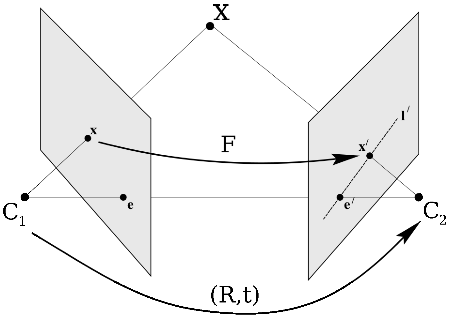
The epipolar geometry can be used to validate the match , since it constrains the position of the points and . As shown in Figure 1, the epipolar line at the point , in the second image, is the intersection of the epipolar plane passing through the optical centers and and the point within the plane of the second image. If the matrix and the point in the first image are known, the epipolar line in the second image where the point is restricted to be, is given by . Similarly, specifies the epipolar line in the first image that corresponds to the point in the second image. This epipolar constraint that restrict the positions of and is used in the proposed method to evaluate candidate solutions by their mapping accuracy.
Given a matrix computed from noisy point correspondences, the quality of the estimated fundamental matrix is evaluated using the epipolar lines. This is done by considering the distance between the points and the epipolar lines to which they must belong. Considering the notation , the distance between the point and the line can be computed as follows:
Likewise, denoting , the other corresponding distance can be calculated as:
To evaluate , a mismatch error produced by the i-correspondence is defined by the sum of squared distances from the points to their corresponding epipolar lines as follows:
2.2.2. Homography
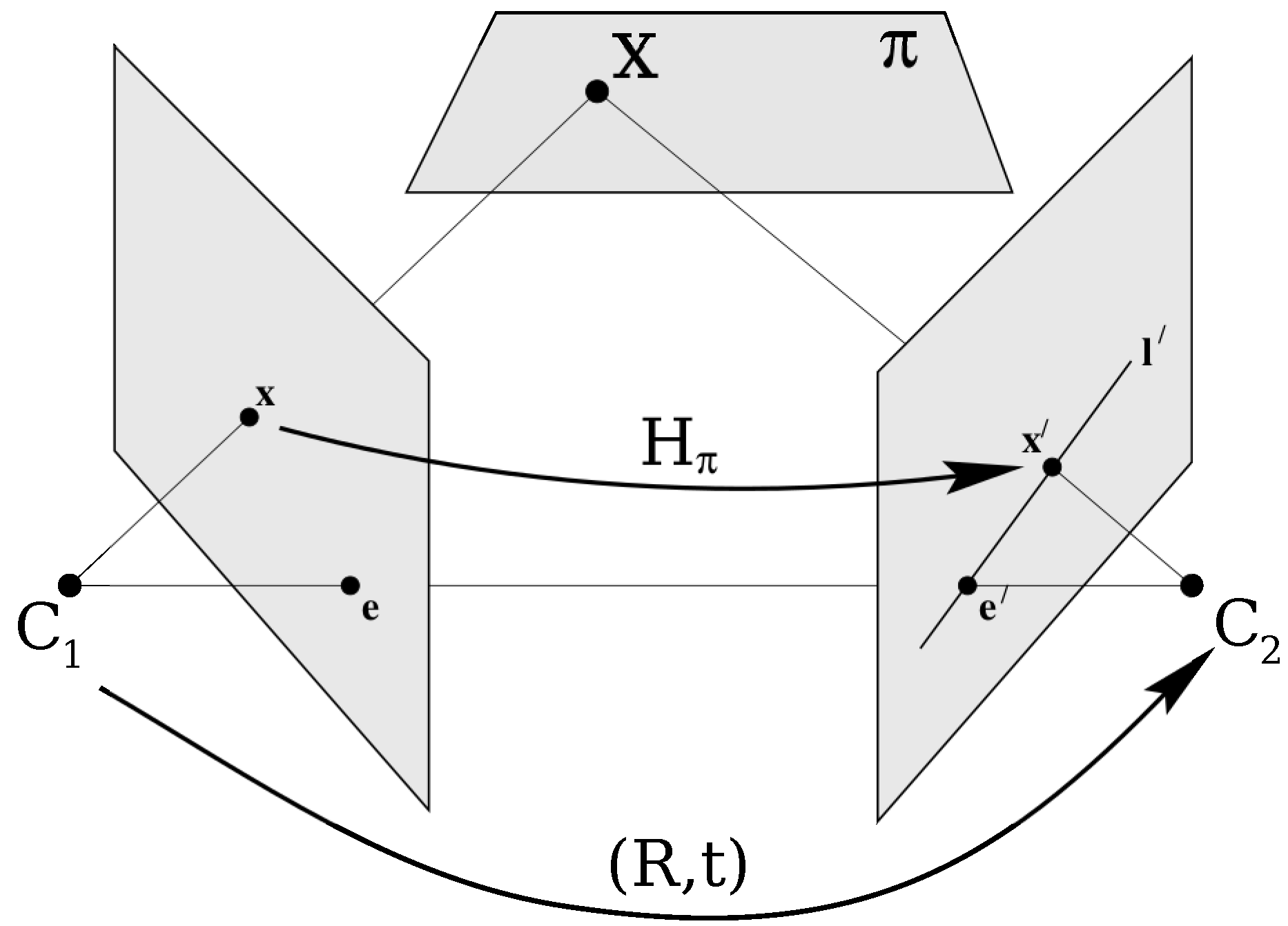
If the match points are said to be in a plane , a homography can be computed. As shown in Figure 2, two perspective images can be geometrically linked through a plane of the scene by a homography . The homography is a projective transformation, and it relates matching or corresponding points belonging to the plane that is projected into two images by or . To find the homography given by two different views, a linear equation system can be generated from a set of four different corresponding points (matches). Then the system can be solved analytically [1].
The computed homography can be evaluated to obtain an accuracy measure. This quality measure can be computed by considering the distance (usually the Euclidean distance) between the position of the point found with the matrix and the actual position of the projection of the observed 3D point. Thereby, the i-correspondence will produce a mismatch error . This error is computed using the sum of squared distances from the estimated point positions to their actual location as stated in following equation
Having described the epipolar geometry, and how a candidate fundamental matrix and homography can be evaluated, we now depict the TLBO algorithm as implemented in the proposed approach.
3. Teaching and Learning Based Optimization Algorithm
The procedure of the TLBO algorithm is based on the metaphor of the teaching and learning processes. First, a population of M students or solutions, S is randomly initialized within the search space. Thus, the initial population is . Each individual , is a real-valued vector with D elements. In the metaphor, D represents the number of assigned subjects a student has, therefore D is the dimension of the problem.
Once the population is initialized the algorithm proceeds to execute the teaching and learning stages. The aim of these two consecutive stages is to enhance the population by modifying individuals. Within the teaching stage, the TLBO algorithm attempts to increase the knowledge (quality) of the population by helping students individually. In the learning stage, on the other hand, the interaction between students is promoted to enhance the quality of the students. The algorithm is carried out until a certain number of iterations.
In the teaching stage, the knowledge transfer is performed by the teacher. Hence within this stage, the individual with the highest fitness value is appointed as the teacher . The TLBO algorithm aims to enhance every other student by moving its position in the teacher direction.
This is done by using the mean value of current population. The locus of student is updated by:
In the above equation, is a real random number, and the teaching factor, is also randomly decided. If has a better quality, i.e., a better fitness value, is replaced by in the population.
As stated by Equation (6), the improvement of the student is affected by both the comparison with the teacher knowledge and the mean quality of all students. The TLBO capabilities of exploration and exploitation are granted by the factors r and . For instance, for the settings of and r near to 1, individuals tend to approximate the teacher. This contributes to the exploitation of the search space surrounding the teacher. Conversely, more exploration in proportion with the r value is performed when .
Finally, during the learner stage, a student tries to improve its fitness value (knowledge) by interacting with an arbitrary student . If is better than , is moved towards accordant with:
If is not better than , is moved away from accordant with:
Similar to the teacher stage, if has a better fitness value, is replaced by in the population.
The TLBO algorithm is a powerful metaheuristic. It solves complex optimization problems yet remaining simple and easy to implement. Therefore, several engineering and scientific applications using this metaheuristic have been published [40,41,42,43]. Differently from the previous work in [44,45,46], this paper proposes a novel application for the TLBO algorithm. Instead of searching for image patterns like the work in [44,45] or detecting vanishing points [46], in this work the TLBO algorithm is implemented for the novel task of estimating the fundamental matrix and homography. The work in [46] deals with the problem of vanishing points detection. While this work tackles the problem of geometric relations encoded in homographies or the fundamental matrix. Although these two problems are different, they can be solved by sampling-based methods such as RANSAC. RANSAC-like methods find models by randomly sampling the search space. Vanishing points can be found by modeling Manhattan frame rotations using sampled image lines. Quite different, the homograpy or fundamental matrix is modeled using RANSAC by sampling candidate matched points. Metaheuristics like the TLBO algorithm also sample the search space, although this sample is not blind but guided by the objective function. In this paper we demonstrate the benefits of metaheuristics over pure random procedures such as RANSAC.
Algorithm 1 depicts the simplest procedure for the process described in this section, which is used in this work for the optimization task of estimating the fundamental matrix and homography as now explained.
| Algorithm 1: Simplest form of the Teaching–Learning-Based Optimization (TLBO) algorithm. |
 |
4. Epipolar Geometry Estimation Using Tlbo
In this section, we depict the utilization of the TLBO algorithm to find multiple view relations, which is a novel task for this metaheuristic. For a metaheuristic to work properly, three different components must be defined: The search space organization, the individual representation, and the objective-function definition. We now describe these elements.
4.1. Search Space
To generate the search space where the TLBO algorithm optimizes, two gray-scale images are processed to find key-features with its corresponding descriptors as described in Section 2. Then, the descriptors are matched using the Euclidean distance in order to find matching pair points . Finally, every pair is added in a set , where M is the number of matches found. For the proposed algorithm to work, it is assumed that the tentative matches in U are consistent with at least one geometric relation model, i.e., a fundamental matrix or a homography. In other words, the two input images are supposed to view the same scene from different viewpoints.
4.2. Individual Representation
In the TLBO-based estimation process, each candidate student S encodes either a homography , or a fundamental matrix . In order to construct a candidate solution or individual that encodes a homography, four indexes are selected from the set of correspondences U. Likewise, in the case of the fundamental matrix, eight indexes are selected from U. A transformation from indexes to either or is done according to Ref. [1].
4.3. Objective Function
In this work, the problem to solve consists in finding the parameters of or through a set of M different noisy correspondences. To find a solution using the TLBO algorithm, this problem is treated as an optimization procedure.
The proposed method implements the TLBO to generate samples or candidate solutions based on information about their quality, rather than randomness as in the case of RANSAC-like algorithms. In the traditional RANSAC method, the classical objective function evaluates only to the number of inliers. Distinctively, we improve results by using a different objective function to accurately evaluate the quality of a candidate model.
The objective function proposed for the TLBO-based estimator uses not only the number of inliers, but also the residual error. Both values are combined into a simple quotient by the following expression:
where represents the quadratic errors or (see Section 2) produced by the jth correspondence considering the candidate transformation or , whereas is defined as follows:
Therefore, the maximization of implies to obtain the candidate solution S having both the highest number of inliers and the lowest residual error, simultaneously. The threshold allows us to assign a number of inliers to a particular candidate solution. When a candidate solution does not map points correctly, the overall quadratic error increases, and the number of outliers must increase as well. Within this work, we have chosen empirically.
The objective function evaluates the quality of a candidate transformation. Guided by the values of this objective function, the set of encoded candidate solutions are modified by using the TLBO process so that they can improve their quality as the optimization process evolves. We now describe the whole process proposed in this work.
4.4. Tlbo for Epipolar Geometry Estimation
The presented approach can be summarized as shown in Figure 3. First, a preprocessing step is carried out to construct the search space. Then, within the initialization procedure of the TLBO algorithm, candidate solutions are randomly generated. After that, the teaching and learning processes of the TLBO algorithm are iteratively executed to improve the quality of the population. Finally, at the end of the predefined number of iterations, the best individual () is selected as the final solution. This solution is used to filter out false matches, i.e., matches not respecting the epipolar restriction. Then, the fundamental-matrix or homography is estimated using all the points in the subset of inliers.
5. Experimental Results
In this section, results of the proposed TLBO-based estimator are reported. A comparison with other approaches is also carried out. The experiments are performed on real images, and the comparisons with the following five different methods: RANSAC as the most recent implementation in OpenCV, MLESAC as implemented in the last version of the Matlab vision toolbox, CSA-RANSAC as implemented in [29] with the same proposed parameters, and an implementation using a Genetic Algorithm (GA), and the Differential Evolution approach (DE) with the same search space and objective function as the TLBO-based estimator.
Images for experimentation are shown in Figure 4, Figure 5, Figure 6 and Figure 7 and 12. Room_1 (640 × 480) and Room_2 (640 × 480) belong to the CIMAT-NAO-A dataset, which was acquired with a NAO humanoid robot. The dataset contains 399 different images with blur effects and low textures. Street_1 (1241 × 376) belongs to the Kitty dataset which is usually used for autonomous driving experiments [47]. Street_2 (1348 × 374), on its part, is taken from the work in [48]. Calibration_rig (690 × 470), Park (720 × 450), and Corridor (370 × 490) are taken from a repository of free images. Finally, Book_1 (671 × 503) and Book_2 (671 × 503) were capture by a generic cellphone camera. The whole set of experiments were carried out on a 2.80 GHz Intel Core i7-7700HQ CPU. The TLBO-based estimator was implemented in C++. Image preparation tasks such as Key-point detection and description were performed by the OpenCV library.
The parameter setup for the metaheuristic approaches, i.e., the TLBO, GA and DE were chosen empirically as usual for metaheuristic methods. The setups are shown in Table 1, Table 2 and Table 3. To perform a fair comparison all metaheuristics were set to execute the same number of objective function evaluations. This particular setting forces the metaheuristics to sample the search space to the same extent. This allows a fair comparison. On the contrary, if a metaheuristic executes more objective function evaluations it gathers more information about the problem, thus having more chances to find a better solution. To compute the objective function, the parameter was empirically determined to 5. All parameters were fixed for the whole set of experiments.
The parameters for the non-metaheuristic methods, i.e., RANSAC and MLESAC were set as follows. Both algorithms need a maximum distance from a point to an epipolar line, and the number of sampling attempts. For the two approaches, the maximum distance was set to 5 pixels similarly to the objective function proposed in Equation (10), and the number of samples equal to the number of objective function evaluations for the metaheuristics estimators.
To show the capabilities of the proposed method for the task of estimating the fundamental matrix , we present Figure 4 and Figure 5. The proposed method also estimates the homography , as shown by the results of Figure 6.
To quantitatively test all methods and compare results, three values are studied: the inlier number , the error , and the residual error, . We first describe the number and the error. Then, results for the residual error are presented.
5.1. Number of Inliers and error
As described in [29,31], the inlier number is used to express the number of detected inliers that are stored in the set . The error, on the other hand, is used to provide a quantitative measure for the quality of the candidate geometric relation. is assessed from the standard deviation of only the inliers. Thus, the error is computed as follows:
where is the quadratic error produced by the i-th inlier. The term corresponds to or as described in Section 2, and represent the errors produced by the ith inlier considering the final fundamental matrix or homography , respectively.
Quantitative results are shown in Table 4 and Table 5. Table 4 exposes the number of inliers and the error for all methods used in Figure 4 and Figure 5. Table 5, on the other hand, shows the results given by the homography for the images in Figure 6.
In three out of four experiments, the TLBO algorithm achieved the smallest error in comparison to the other methods. It was only in the case of the Room_1 image that the GA-based estimator outperformed slightly the TLBO algorithm in terms of the error by 0.01. However, The TLBO algorithm found a greater number of inliers, i.e., matched points within 5 pixels distant from its corresponding epipolar line.
The different performance of each method is linked with its approach to solve the problem. The RANSAC and MLESAC perform a random sampling within the search space, while the metaheuristic-based estimators carried out a guided search. RANSAC-like methods try many different random subsets of the corresponding point matches, and estimate the model using this subset to solve the system. Finally, the best subset is then used to produce the final model that will filter out wrong matches. To achieve this, RANSAC-based methods perform a model computation from point correspondences, and compute an error to rank and compare subsets. The TLBO algorithm, on the other hand, leverages of this error computation to guide the search in order to perform a better space search.
In the experiments, all the methods start with the same set of point correspondences. This set contains both good and bad matches. The non-metaheuristic methods are constrained to sample the search space an equal number of times as the metaheuristic approaches. Given that the former methods are purely random, the less they sample the space, the greater the probability of giving a wrong model. In the case of the metaheuristic approaches, the capability of finding an accurate model resides in the exploration and exploitation capacities of the method. Each metaheuristic can be tuned to modify the exploration and exploitation of the search space. The advantage of the TLBO algorithm resides in that it has fewer parameters to tune, still keeping its accurate performance.
To further show the performance of the proposed method as compared to other approaches, the residual error is computed for the fundamental matrix estimation, and a comparison of correct matched points using the homography is perform.
5.2. Residual Error
Accurate estimation of epipolar entities is important for multiple applications. For instance, camera calibration and 3D reconstruction rely on a nonlinear cost function defined from the relationship between the projection matrices and fundamental matrices. Vision-based control of robots and global motion compensation depend on homography transformations between consecutive frames. Since epipolar correlations are determined from the matched points, these applications strive when only a few points are available. Lack of data is present when there are appearance ambiguities, multi-plane scenes, and dominant dynamic features instead of static features. To show the capabilities of the proposed approach to accurately estimate epipolar entities with few data, we compute the residual error, :
where is the distance in pixels between point and line . The error is the squared distance between an epipolar line and the matching point in the other image, average over all N matches. This particular error is not minimized directly by any of the algorithms.
For the experimental procedure, each pair of images is preprocessed as in Section 4 to found a set of noisy matched points U. Then, a number n of matched points are chosen randomly from U. Finally, the fundamental matrix is estimated, and the residual error computed. The residual error is evaluated over all N matched points, and not just the n matches used to compute . The set of images for experimentation is shown in Figure 7.
The aforementioned procedure was repeated 100 times for each value of n and each pair of images. The average residual error is plotted against n in Figure 8, Figure 9, Figure 10 and Figure 11. Likewise, this values are shown in Table 6, Table 7, Table 8 and Table 9. This gives an idea of how the different algorithms behave as the number of points increases.
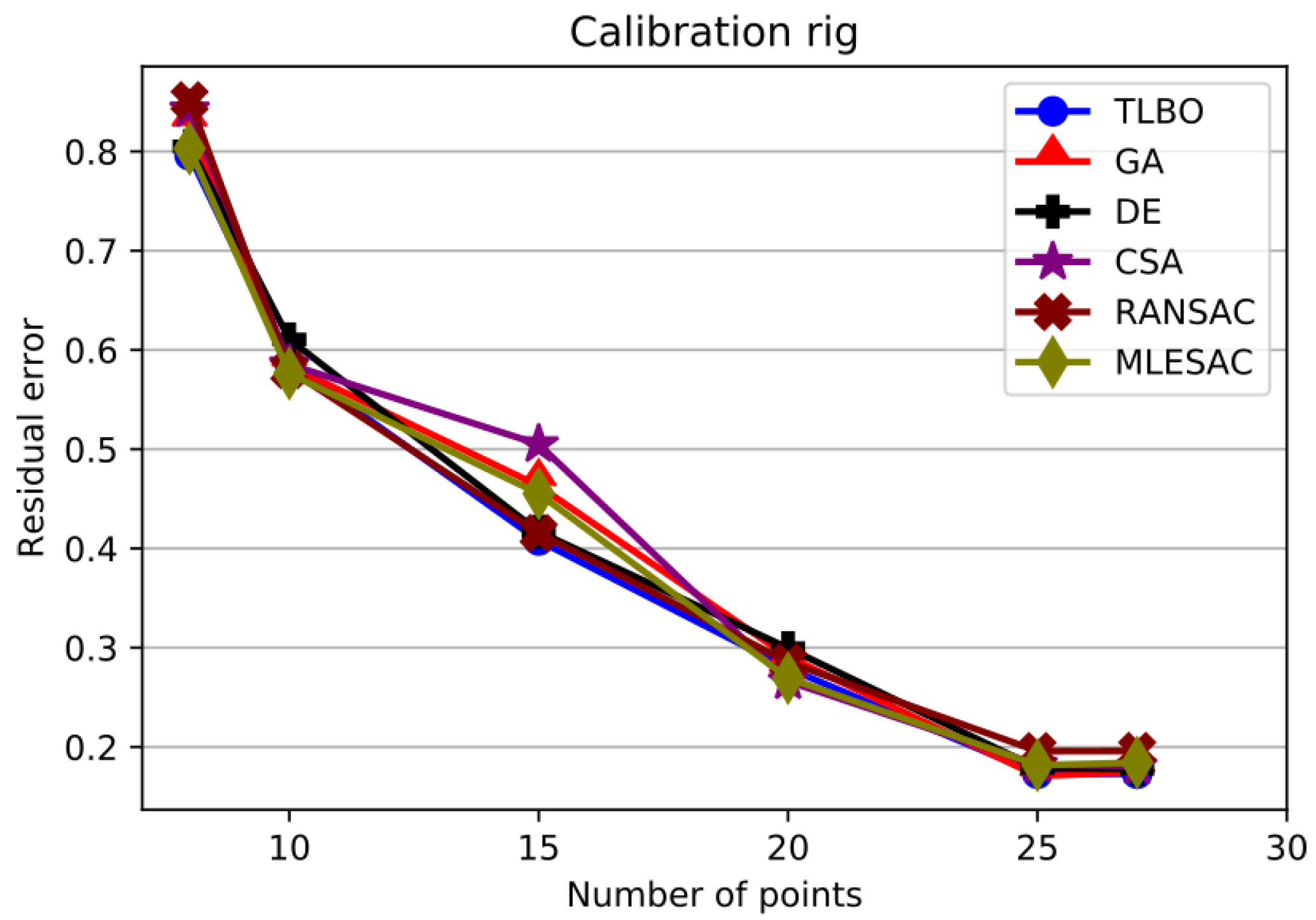
As shown in Figure 8, the error for the Calibration rig is the smallest over the whole set of experiments. This is because the matched points were known precisely. As indicated in Table 6, however, the TLBO algorithm attained a better error in more cases than the rest of the methods. From these results, it can be said that for this experiment a metaheuristic approach guided by the objective function performs better than a purely random procedure.
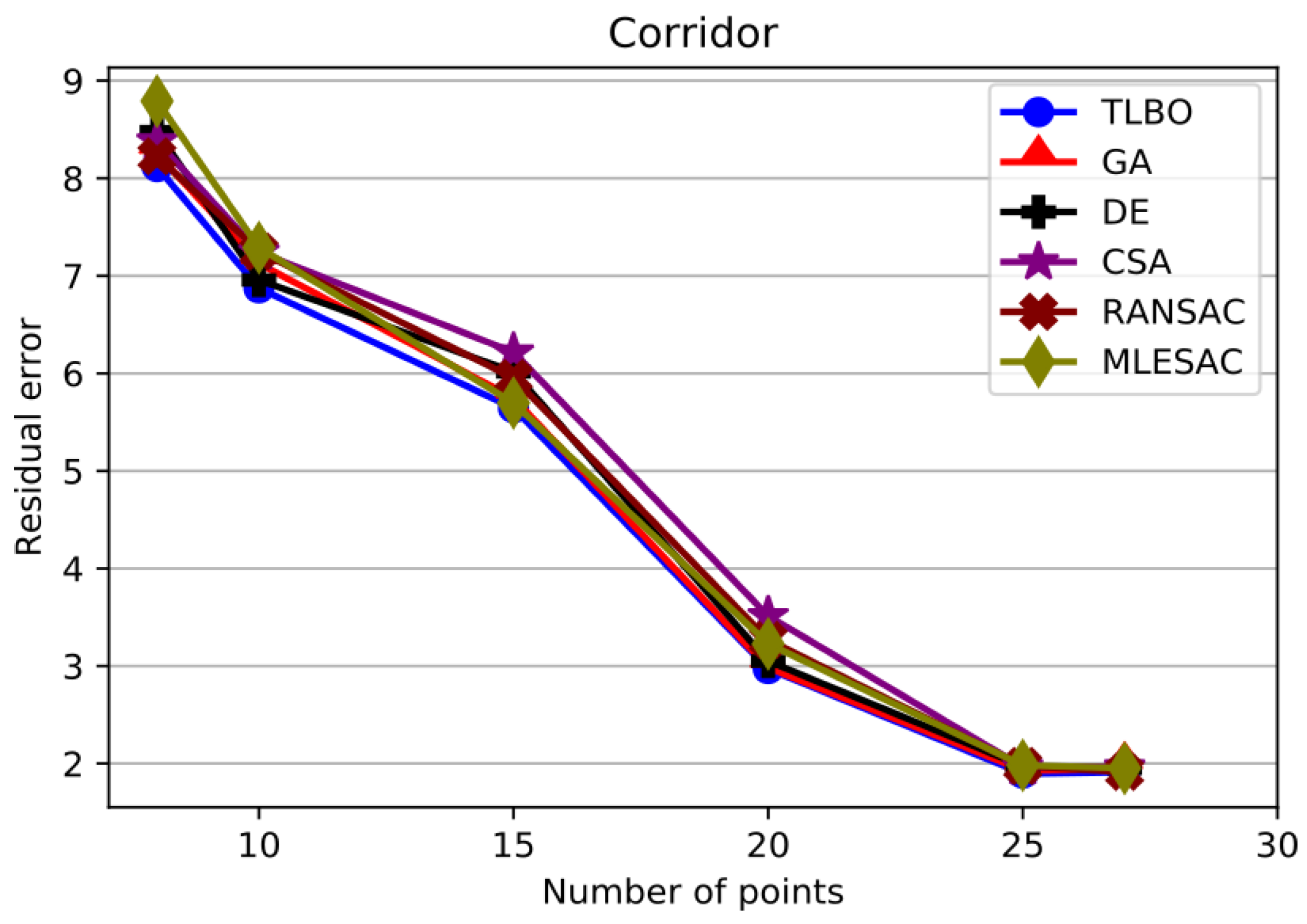
When images get more complicated, the TLBO algorithm outstands from the rest of the methods. For the Park image shown in Figure 9, for instance, the proposed method excels with a smaller error for each value of n. The same is the case for the Corridor image as shown in Figure 10.
Results from the Book image are depicted in Figure 11. In this case, the TLBO algorithm attained a better error overall. Only for n = 15 it was outperformed slightly by the GA-based estimator by 0.007. The cause for the different performance is the searching procedure each algorithm performs. RANSAC, and its variation MLESAC, sample the data randomly to choose the model with the most votes. The TLBO algorithm, on the other hand, guides the search by minimizing an objective function and performing particular operations in the candidate solutions to move them towards the best solution. This permits the TLBO algorithm to achieve a smaller error with less sampling executions.
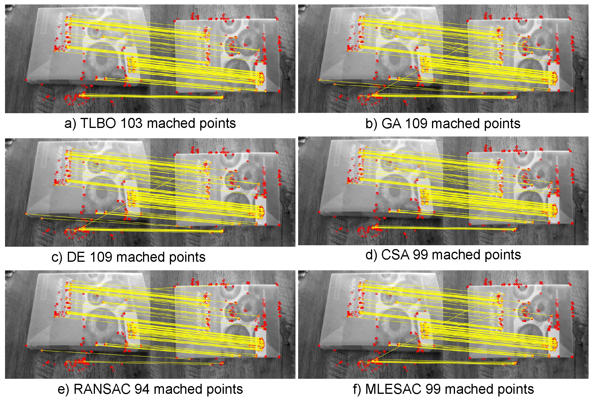
An accurate estimation of a fundamental matrix or homography is also used to filter out false matches. Regarding the homography estimation, Figure 12 depicts results for the computation of the homography. As shown in the figure, the TLBO algorithm found 103 true positive matched points, while the other methods found either less true points or more false positives. As can be concluded by the experiments, the TLBO algorithm is and efficient metaheuristic for estimating epipolar entities.
The comparison experiments with the whole set of methods involved the task of finding the smallest error given the same threshold (maximum distance in pixels for a point to be considered an inlier), and the same possibility of space search. Feature detection was performed to sub-pixel accuracy, which allowed us to compare in this scale. As shown from the results, the TLBO-based estimator outperformed the rest of the methods overall. The reason for this outcome lies in the capabilities of the TLBO. The proposed method does not require many sampling executions because it explores and exploits the search space in a metaheuristic fashion. It also optimizes over the search space guided by a detailed objective function.
Since we constrained the number of samples every method can perform, the RANSAC-like methods performed poorly. This is because, ideally, the threshold should be computed assuming the measurement error Gaussian with zero mean, and the number of samples according to the proportion of outliers. Even when the MLESAC algorithm differs from RANSAC in the error definition, it adopts the same sampling strategy as RANSAC to generate putative solutions, thus it suffers if the number of samples is set to low.
Another reason for the proposed method to outperform the RANSAC-like methods is the definition of the objective function. RANSAC chooses the solution that maximizes the number of inliers, and MLESAC chooses the solution that maximizes the likelihood. The proposed method, on the other hand, is guided by an accurate objective function that takes into account both the number of inliers and the residual of the quadratic error.
Regarding the other metaheuristics, the TLBO algorithm performed better in comparison to the DE and CSA methods. The GA-based estimator outperformed slightly the TLBO algorithm in 3 different cases. However, given that the objective of this work is to present a method that accurately estimates epipolar entities without the need to adjust various parameters for different kinds of images, the proposed approach achieved this task better than the other metaheuristic methods. Differently from the other metaheuristic-based estimators, the TLBO algorithm does not need the tuning of any algorithm-specific parameters.
6. Conclusions
This work tackles the problem of computing the fundamental matrix and homography using the TLBO algorithm. The task of finding multiple view geometric relations is a novel application of the TLBO metaheuristic. The proposed approach is a robust method for estimating the epipolar geometry in spite of poorly matched points. The TLBO-based solution computes the best model for the homography or fundamental matrix, and at the same time it filters out wrong point correspondences. Instead of being purely random as RANSAC-like methods, the proposed approach improves the computed solution by performing a metaheuristic search by using the TLBO algorithm.
Differently from the pure random strategy that the RANSAC algorithm performs, the proposed approach, guided by the TLBO algorithm, builds iteratively new potential solutions considering previously generated candidate individuals. The method takes into consideration the quality of these solutions. Furthermore, the proposed method uses a better objective function.
To certainly evaluate the quality of a candidate model (solution), the used objective function uses both the number of inliers and the residual error. As a result of this approach, a considerable reduction of the number of iterations in comparison with RANSAC is achieved, still maintaining the robustness capability of RANSAC. Future work can be directed towards the metaheuristic solution of the non-linear cases of the epipolar geometry.
Author Contributions
Conceptualization, methodology, software, validation, formal analysis, investigation, writing—original draft preparation, A.L.-M.; writing—review and editing, Supervision, F.J.C. All authors have read and agreed to the published version of the manuscript.
Funding
This research received no external funding.
Conflicts of Interest
The authors declare no conflict of interest that could have appeared to influence the work reported in this paper.
References
- Hartley, R.; Zisserman, A. Multiple View Geometry in Computer Vision; Cambridge University Press: Cambridge, UK, 2003. [Google Scholar]
- Xia, M.; Yao, J.; Xie, R.; Li, L.; Zhang, W. Globally consistent alignment for planar mosaicking via topology analysis. Pattern Recognit. 2017, 66, 239–252. [Google Scholar] [CrossRef]
- Zhang, Y.; Lai, Y.K.; Zhang, F.L. Stereoscopic image stitching with rectangular boundaries. Vis. Comput. 2019, 35, 823–835. [Google Scholar] [CrossRef]
- Park, K.w.; Shim, Y.J.; Lee, M.J.; Ahn, H. Multi-Frame Based Homography Estimation for Video Stitching in Static Camera Environments. Sensors 2020, 20, 92. [Google Scholar] [CrossRef] [Green Version]
- D’Orazio, T.; Guaragnella, C. A survey of automatic event detection in multi-camera third generation surveillance systems. Int. J. Pattern Recognit. Artif. Intell. 2015, 29, 1555001. [Google Scholar] [CrossRef]
- El Akkad, N.; Merras, M.; Saaidi, A.; Satori, K. Camera self-calibration with varying intrinsic parameters by an unknown three-dimensional scene. Vis. Comput. 2014, 30, 519–530. [Google Scholar] [CrossRef] [Green Version]
- Montijano, E.; Cristofalo, E.; Zhou, D.; Schwager, M.; Saguees, C. Vision-based distributed formation control without an external positioning system. IEEE Trans. Robot. 2016, 32, 339–351. [Google Scholar] [CrossRef]
- Ullah, H.; Zia, O.; Kim, J.H.; Han, K.; Lee, J.W. Automatic 360 Mono-Stereo Panorama Generation Using a Cost-Effective Multi-Camera System. Sensors 2020, 20, 3097. [Google Scholar] [CrossRef] [PubMed]
- El Hazzat, S.; Merras, M.; El Akkad, N.; Saaidi, A.; Satori, K. 3D reconstruction system based on incremental structure from motion using a camera with varying parameters. Vis. Comput. 2018, 34, 1443–1460. [Google Scholar] [CrossRef]
- Töberg, S.; Reithmeier, E. Quantitative 3D Reconstruction from Scanning Electron Microscope Images Based on Affine Camera Models. Sensors 2020, 20, 3598. [Google Scholar] [CrossRef]
- Safdarnejad, S.M.; Atoum, Y.; Liu, X. Temporally robust global motion compensation by keypoint-based congealing. In European Conference on Computer Vision; Springer: Berlin/Heidelberg, Germany, 2016; pp. 101–119. [Google Scholar]
- Kanojia, G.; Raman, S. Patch-based detection of dynamic objects in CrowdCam images. Vis. Comput. 2019, 35, 521–534. [Google Scholar] [CrossRef]
- Cleju, I.; Saupe, D. Evaluation of texture registration by epipolar geometry. Vis. Comput. 2010, 26, 1407–1420. [Google Scholar] [CrossRef] [Green Version]
- Delfin, J.; Becerra, H.M.; Arechavaleta, G. Humanoid localization and navigation using a visual memory. In Proceedings of the 2016 IEEE-RAS 16th International Conference on Humanoid Robots (Humanoids), Cancun, Mexico, 15–17 November 2016; IEEE: Piscataway, NJ, USA, 2016; pp. 725–731. [Google Scholar]
- Delfin, J.; Becerra, H.M.; Arechavaleta, G. Humanoid navigation using a visual memory with obstacle avoidance. Robot. Auton. Syst. 2018, 109, 109–124. [Google Scholar] [CrossRef]
- López-Martínez, A.; Cuevas, F.; Sosa-Balderas, J. Visual Memory Construction for Autonomous Humanoid Robot Navigation. In Progress in Optomechatronic Technologies; Springer: Berlin/Heidelberg, Germany, 2019; pp. 103–109. [Google Scholar]
- Wu, Z.; Zhou, Z.; Tian, D.; Wu, W. Reconstruction of three-dimensional flame with color temperature. Vis. Comput. 2015, 31, 613–625. [Google Scholar] [CrossRef] [Green Version]
- Simon, G.; Berger, M.O. Interactive building and augmentation of piecewise planar environments using the intersection lines. Vis. Comput. 2011, 27, 827–841. [Google Scholar] [CrossRef] [Green Version]
- Zhang, Y.; Zhou, L.; Shang, Y.; Zhang, X.; Yu, Q. Contour model based homography estimation of texture-less planar objects in uncalibrated images. Pattern Recognit. 2016, 52, 375–383. [Google Scholar] [CrossRef]
- Saputra, M.R.U.; Markham, A.; Trigoni, N. Visual SLAM and structure from motion in dynamic environments: A survey. ACM Comput. Surv. 2018, 51, 37. [Google Scholar] [CrossRef]
- Liu, S.; Chen, J.; Chang, C.H.; Ai, Y. A new accurate and fast homography computation algorithm for sports and traffic video analysis. IEEE Trans. Circuits Syst. Video Technol. 2018, 28, 2993–3006. [Google Scholar] [CrossRef]
- Du, W.L.; Li, X.Y.; Ye, B.; Tian, X.L. A Fast Dense Feature-Matching Model for Cross-Track Pushbroom Satellite Imagery. Sensors 2018, 18, 4182. [Google Scholar] [CrossRef] [Green Version]
- Zhang, Z.; Deriche, R.; Faugeras, O.; Luong, Q.T. A robust technique for matching two uncalibrated images through the recovery of the unknown epipolar geometry. Artif. Intell. 1995, 78, 87–119. [Google Scholar] [CrossRef] [Green Version]
- Pollefeys, M.; Koch, R.; Van Gool, L. Self-calibration and metric reconstruction inspite of varying and unknown intrinsic camera parameters. Int. J. Comput. Vis. 1999, 32, 7–25. [Google Scholar] [CrossRef]
- Hartley, R.; Zisserman, A. Epipolar geometry and the fundamental matrix. Mult. View Geom. 2000, 9, 239–261. [Google Scholar]
- Furukawa, Y.; Ponce, J. Accurate, dense, and robust multiview stereopsis. IEEE Trans. Pattern Anal. Mach. Intell. 2010, 32, 1362–1376. [Google Scholar] [CrossRef] [PubMed]
- Roberts, R.; Sinha, S.N.; Szeliski, R.; Steedly, D. Structure from motion for scenes with large duplicate structures. In Proceedings of the CVPR 2011, Providence, RI, USA, 20–25 June 2011; IEEE: Piscataway, NJ, USA, 2011; pp. 3137–3144. [Google Scholar]
- Fischler, M.A.; Bolles, R.C. Random sample consensus: A paradigm for model fitting with applications to image analysis and automated cartography. Commun. ACM 1981, 24, 381–395. [Google Scholar] [CrossRef]
- Cuevas, E.; Zaldívar, D.; Perez-Cisneros, M. Estimation of Multiple View Relations Considering Evolutionary Approaches. In Applications of Evolutionary Computation in Image Processing and Pattern Recognition; Springer: Berlin/Heidelberg, Germany, 2016; pp. 107–138. [Google Scholar]
- Cuevas, E.; Díaz, M. A method for estimating view transformations from image correspondences based on the harmony search algorithm. Comput. Intell. Neurosci. 2015, 2015, 434263. [Google Scholar] [CrossRef] [PubMed] [Green Version]
- Cuevas, E.; Osuna, V.; Oliva, D. Estimation of View Transformations in Images. In Evolutionary Computation Techniques: A Comparative Perspective; Springer: Berlin/Heidelberg, Germany, 2017; pp. 181–204. [Google Scholar]
- Harris, C.G.; Stephens, M. A combined corner and edge detector. In Alvey Vision Conference; Elsevier: Amsterdam, The Netherlands, 1988; Volume 15, pp. 10–5244. [Google Scholar]
- Lowe, D.G. Distinctive image features from scale-invariant keypoints. Int. J. Comput. Vis. 2004, 60, 91–110. [Google Scholar] [CrossRef]
- Bay, H.; Tuytelaars, T.; Van Gool, L. Surf: Speeded up robust features. In European Conference on Computer Vision; Springer: Berlin/Heidelberg, Germany, 2006; pp. 404–417. [Google Scholar]
- Rosten, E.; Drummond, T. Machine learning for high-speed corner detection. In European Conference on Computer Vision; Springer: Berlin/Heidelberg, Germany, 2006; pp. 430–443. [Google Scholar]
- Calonder, M.; Lepetit, V.; Strecha, C.; Fua, P. Brief: Binary robust independent elementary features. In European Conference on Computer Vision; Springer: Berlin/Heidelberg, Germany, 2010; pp. 778–792. [Google Scholar]
- Rublee, E.; Rabaud, V.; Konolige, K.; Bradski, G.R. ORB: An efficient alternative to SIFT or SURF. In Proceedings of the 2011 International Conference on Computer Vision, Barcelona, Spain, 6–13 November 2011; Volume 11, p. 2. [Google Scholar]
- Huynh, D.Q.; Saini, A.; Liu, W. Evaluation of three local descriptors on low resolution images for robot navigation. In Proceedings of the 2009 24th International Conference Image and Vision Computing New Zealand, Wellington, New Zealand, 23–25 November 2009; IEEE: Piscataway, NJ, USA, 2009; pp. 113–118. [Google Scholar]
- Hartley, R. In Defense of the Eight Point Algorithm. In IEEE Transactions on Pattern Analysis and Machine Intelligence; IEEE: Piscataway, NJ, USA, 1997. [Google Scholar]
- Rao, R.V.; Savsani, V.J.; Vakharia, D. Teaching–learning-based optimization: A novel method for constrained mechanical design optimization problems. Comput. Aided Des. 2011, 43, 303–315. [Google Scholar] [CrossRef]
- Rao, R. Review of applications of TLBO algorithm and a tutorial for beginners to solve the unconstrained and constrained optimization problems. Decis. Sci. Lett. 2016, 5, 1–30. [Google Scholar]
- Goyal, R.K.; Kaushal, S. A constrained non-linear optimization model for fuzzy pairwise comparison matrices using teaching learning based optimization. Appl. Intell. 2016, 45, 652–661. [Google Scholar] [CrossRef]
- El Ghazi, A.; Ahiod, B. Energy efficient teaching-learning-based optimization for the discrete routing problem in wireless sensor networks. Appl. Intell. 2018, 48, 2755–2769. [Google Scholar] [CrossRef]
- López, A.; Cuevas, F.J. Automatic multi-circle detection on images using the teaching learning based optimisation algorithm. IET Comput. Vis. 2018, 12, 1188–1199. [Google Scholar] [CrossRef]
- Lopez-Martinez, A.; Cuevas, F.J. Automatic circle detection on images using the Teaching Learning Based Optimization algorithm and gradient analysis. Appl. Intell. 2019, 49, 2001–2016. [Google Scholar] [CrossRef]
- López-Martinez, A.; Cuevas, F.J. Vanishing point detection using the teaching learning-based optimisation algorithm. IET Image Process. 2020, 14, 2487–2494. [Google Scholar] [CrossRef]
- Geiger, A.; Lenz, P.; Urtasun, R. Are we ready for autonomous driving? the kitti vision benchmark suite. In Proceedings of the 2012 IEEE Conference on Computer Vision and Pattern Recognition, Providence, RI, USA, 16–21 June 2012; IEEE: Piscataway, NJ, USA, 2012; pp. 3354–3361. [Google Scholar]
- Garcia-Fidalgo, E.; Ortiz, A. Probabilistic appearance-based mapping and localization using visual features. In Iberian Conference on Pattern Recognition and Image Analysis; Springer: Berlin/Heidelberg, Germany, 2013; pp. 277–285. [Google Scholar]
Figure 1.
Epipolar geometry depiction: the fundamental matrix case. Two cameras, and , are viewing the same scene. Both cameras are represented by their centres, and image plane. As shown in the figure, the centres, and lie in the same plane as the 3D point X and its images x and . The point correspondence geometry is constrained as follows. The image point x back-projects to a ray in 3D space defined by the first camera centre, , and x. As can be seen, the 3D point X which projects to x must lie on this ray. Since the image of this ray, is the line in the second view, the image of X in the second view must lie on

Figure 2.
Epipolar geometry depiction: The Homography case. A point x in one image is transferred, differently from the fundamental-matrix case, via the plane to a matching point in the second image. The epipolar line through is obtained by joining to the epipole
Figure 2.
Epipolar geometry depiction: The Homography case. A point x in one image is transferred, differently from the fundamental-matrix case, via the plane to a matching point in the second image. The epipolar line through is obtained by joining to the epipole

Figure 3.
Teaching–Learning-Based Optimization (TLBO)-based process for estimating geometric relations. Three main steps are followed in order to compute the geometric relations given by either the fundamental matrix or the homography. First, a preprocessing step is carried out to compute the search space. Then, the TLBO population is initialized according to the constrains of the problem. Finally, the TLBO learning process is iteratively executed to find the final solution, i.e., a fundamental matrix or a homography.

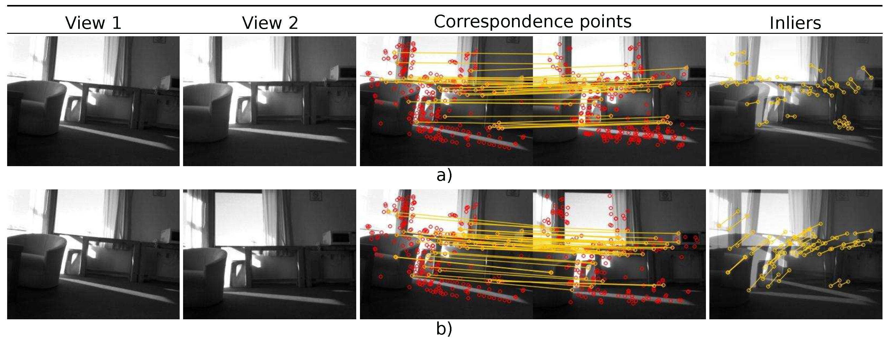
Figure 4.
Results for the fundamental-matrix estimation from test images (a) Room_1 and (b) Room_2. The first and second columns show the first and second view, respectively. The third column shows the correspondence points along with outliers contained in the dataset. The fourth column depicts a blended image of the two views with inliers found by the proposed method.

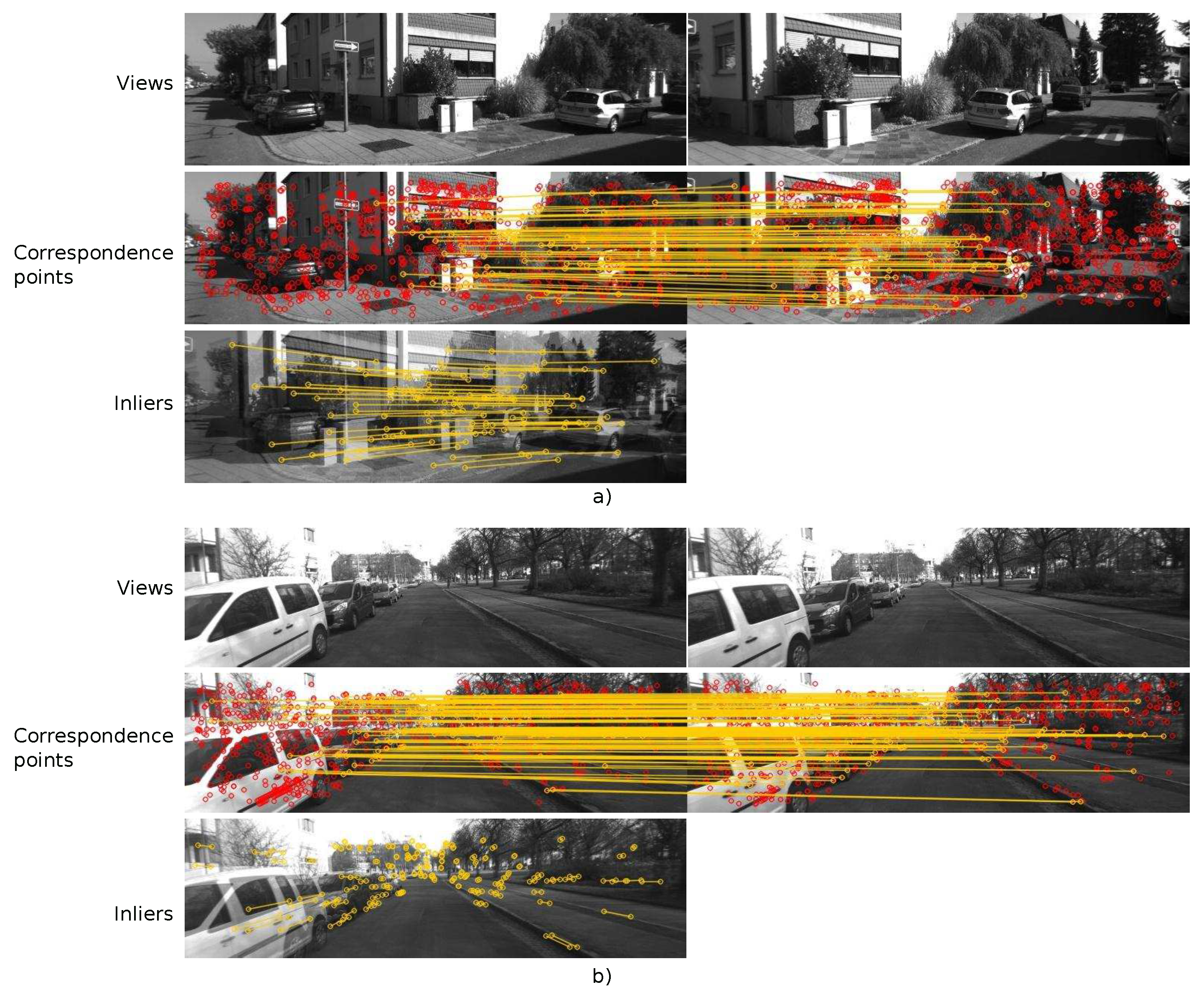
Figure 5.
Results for the fundamental-matrix estimation from test images (a) Street_1 and (b) Street_2. The first row shows the first and second view. The second row shows the correspondence points along with outliers contained in the dataset. The third row depicts a blended image of the two views with inliers found by the proposed method.

Figure 6.
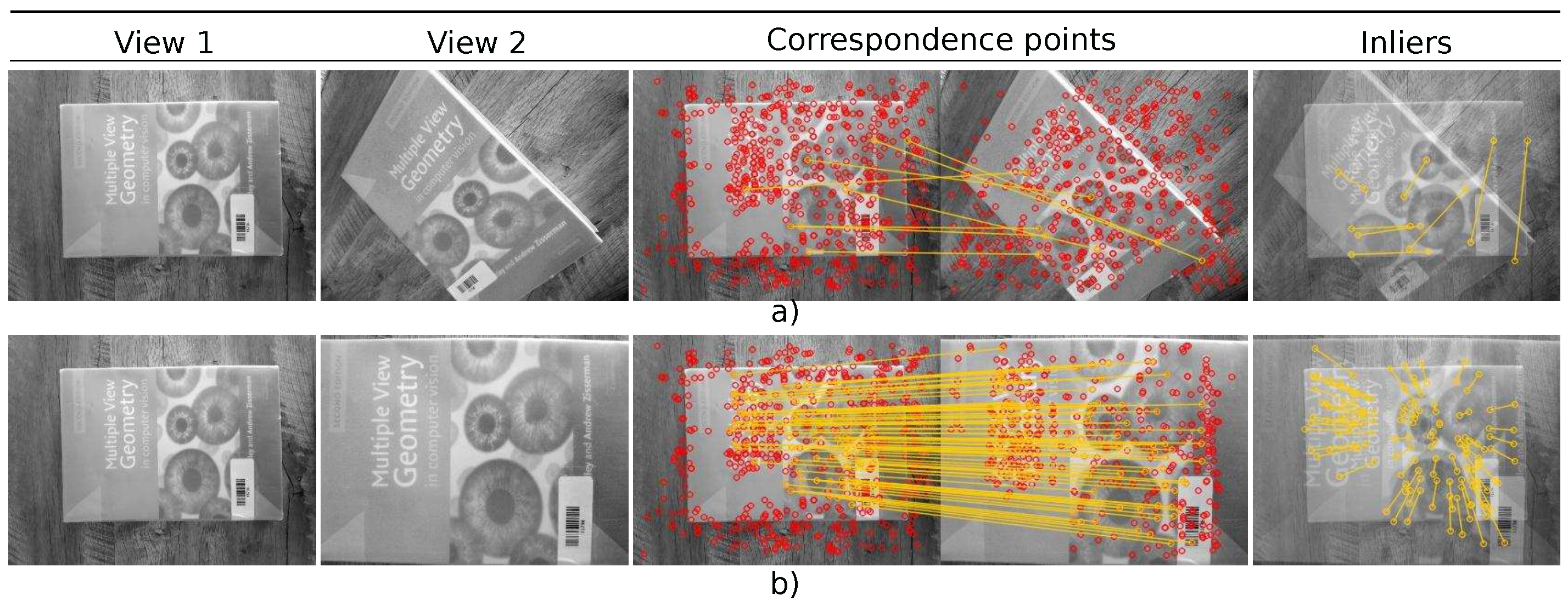
Results for the homography estimation from the test images (a) Book_1 and (b) Book_2. The first and second columns show the first and second view, respectively. The third column shows the correspondence points along with outliers contained in the dataset. The fourth column depicts a blended image of the two views with inliers found by the proposed method.
Figure 6.
Results for the homography estimation from the test images (a) Book_1 and (b) Book_2. The first and second columns show the first and second view, respectively. The third column shows the correspondence points along with outliers contained in the dataset. The fourth column depicts a blended image of the two views with inliers found by the proposed method.

Figure 7.
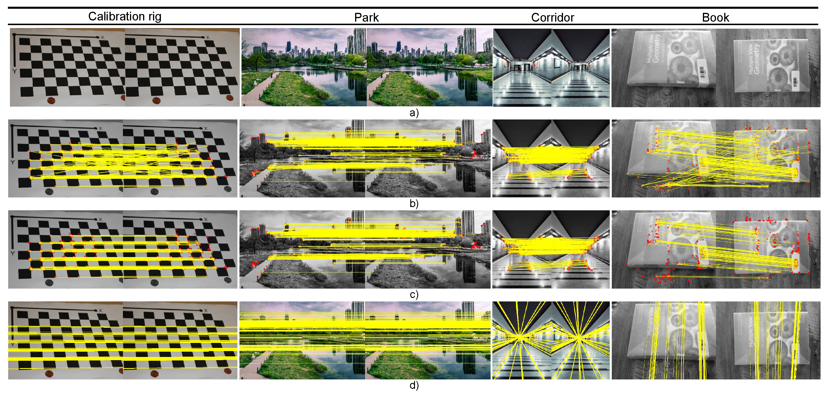
Image pairs for algorithm comparison. With and estimated fundamental matrix, epipole lines can be computed. The whole set of accurate matched points should be close to its corresponding epipole line. (a) The pair of original images. (b) The Euclidian-based matches. (c) The inlier points consistent with the epipolar restriction as found by the proposed method. (d) The epipolar lines (25% of the lines are depicted in the image).
Figure 7.
Image pairs for algorithm comparison. With and estimated fundamental matrix, epipole lines can be computed. The whole set of accurate matched points should be close to its corresponding epipole line. (a) The pair of original images. (b) The Euclidian-based matches. (c) The inlier points consistent with the epipolar restriction as found by the proposed method. (d) The epipolar lines (25% of the lines are depicted in the image).

Figure 8.
Results of the experimental evaluation of the methods for computing the fundamental matrix for the Calibration rig image in Figure 7. In each case, six different approaches are compared. For the experiment, n number of points are used to search for a fundamental matrix. For each n, 100 experiments were carried out and the residual error averaged.

Figure 9.
Results of the experimental evaluation of the methods for computing the fundamental matrix for the Park image in Figure 7. In each case, six different approaches are compared. For the experiment, n number of points are used to search for a fundamental matrix. For each n, 100 experiments were carried out and the residual error averaged.

Figure 10.
Results of the experimental evaluation of the methods for computing the fundamental matrix for the Corridor image in Figure 7. In each case, six different approaches are compared. For the experiment, n number of points are used to search for a fundamental matrix. For each n, 100 experiments were carried out and the residual error averaged.

Figure 11.
Results of the experimental evaluation of the methods for computing the fundamental matrix for the Book image in Figure 7. In each case, six different approaches are compared. For the experiment, n number of points are used to search for a fundamental matrix. For each n, 100 experiments were carried out and the residual error averaged.

Figure 12.
Results of the experimental evaluation of the methods for computing a homography. For each image, the number of matched points is shown. The GA and DE estimators found more matched points. However, some of them are false detections. Clonal Selection Algorithm (CSA), Random Sample Consensus (RANSAC) and MLESAC also detect false positives. The TLBO, on the other hand, detected 103 true positive matched points.


Table 1.
Parameter setup for the TLBO-based estimator.
| Parameter | Value |
|---|---|
| Iterations | 100 |
| Population size | 50 |
Table 2.
Parameter setup for the Genetic Algorithm (GA)-based estimator.
| Parameter | Value |
|---|---|
| Number of generations | 201 |
| Population size | 50 |
| Crossover rate | 0.85 |
| Mutation rate | 0.10 |
| Selection method | Roulette with sigma scaling |
| Crossover method | 1-point crossover |
Table 3.
Parameter setup for the Differential Evolution (DE)-based estimator.
| Parameter | Value |
|---|---|
| Number of epochs | 200 |
| Population size | 50 |
| Differential weight | 0.25 |
| Crossover probability | 0.80 |
Table 4.
Number of inliers IN and error Er for all approaches using images in Figure 4 and Figure 5. The best result is highlighted in bold.
| Image | TLBO-Based | GA-Based | DE-Based | CSA-Based | RANSAC | MLESAC | ||||||
|---|---|---|---|---|---|---|---|---|---|---|---|---|
| IN | Er Error | IN | Er Error | IN | Er Error | IN | Er Error | IN | Er Error | IN | Er Error | |
| Room_1 | 47 | 0.86 | 42 | 0.85 | 45 | 1.12 | 47 | 0.78 | 46 | 2.80 | 43 | 2.36 |
| Room_2 | 42 | 0.75 | 45 | 1.24 | 45 | 1.03 | 45 | 1.29 | 43 | 2.45 | 39 | 1.76 |
| Street_1 | 64 | 0.61 | 59 | 0.91 | 58 | 0.83 | 62 | 1.03 | 62 | 1.75 | 67 | 1.85 |
| Street_2 | 127 | 0.91 | 115 | 1.01 | 110 | 1.24 | 110 | 1.52 | 98 | 2.54 | 95 | 2.67 |
Table 5.
Number of inliers IN and error Er for all approaches, considering the test images in Figure 6. The best result is highlighted in bold.
Table 5.
Number of inliers IN and error Er for all approaches, considering the test images in Figure 6. The best result is highlighted in bold.
| Image | TLBO-Based | GA-Based | DE-Based | CSA-Based | RANSAC | MLESAC | ||||||
|---|---|---|---|---|---|---|---|---|---|---|---|---|
| IN | Er Error | IN | Er Error | IN | Er Error | IN | Er Error | IN | Er Error | IN | Er Error | |
| Book_1 | 8 | 0.25 | 8 | 0.78 | 8 | 0.85 | 8 | 0.64 | 8 | 1.068 | 8 | 1.84 |
| Book_2 | 71 | 0.42 | 73 | 0.63 | 71 | 0.51 | 71 | 0.73 | 68 | 1.07 | 63 | 1.36 |
Table 6.
Data points for the experiment with the Calibration rig image of Figure 7. The number n of points for model estimation and the average residual error Eres for all methods are shown. The best result is highlighted in bold.
Table 6.
Data points for the experiment with the Calibration rig image of Figure 7. The number n of points for model estimation and the average residual error Eres for all methods are shown. The best result is highlighted in bold.
| n | TLBO | GA | DE | CSA | RANSAC | MLESAC |
|---|---|---|---|---|---|---|
| Average Er | Average Er | Average Er | Average Er | Average Er | Average Er | |
| 8 | 0.796 | 0.825 | 0.805 | 0.842 | 0.851 | 0.802 |
| 10 | 0.587 | 0.583 | 0.610 | 0.585 | 0.579 | 0.576 |
| 15 | 0.408 | 0.463 | 0.416 | 0.504 | 0.415 | 0.455 |
| 20 | 0.279 | 0.282 | 0.299 | 0.286 | 0.285 | 0.269 |
| 25 | 0.173 | 0.171 | 0.178 | 0.182 | 0.195 | 0.181 |
| 27 | 0.173 | 0.174 | 0.177 | 0.180 | 0.195 | 0.184 |
Table 7.
Data points for the experiment with the Park image of Figure 7. The number n of points for model estimation and the average residual error Eres for all methods are shown. The best result is highlighted in bold.
Table 7.
Data points for the experiment with the Park image of Figure 7. The number n of points for model estimation and the average residual error Eres for all methods are shown. The best result is highlighted in bold.
| n | TLBO | GA | DE | CSA | RANSAC | MLESAC |
|---|---|---|---|---|---|---|
| Average Er | Average Er | Average Er | Average Er | Average Er | Average Er | |
| 8 | 22.127 | 22.784 | 22.752 | 23.446 | 22.685 | 23.560 |
| 10 | 15.524 | 17.285 | 15.553 | 15.722 | 16.048 | 15.595 |
| 15 | 12.183 | 13.757 | 13.573 | 14.554 | 12.197 | 12.694 |
| 20 | 9.220 | 9.912 | 9.434 | 8.965 | 10.064 | 9.164 |
| 25 | 2.214 | 2.224 | 2.507 | 2.267 | 2.248 | 2.486 |
| 27 | 2.197 | 2.633 | 2.352 | 2.585 | 2.442 | 2.256 |
Table 8.
Data points for the experiment with the Corridor image of Figure 7. The number n of points for model estimation and the average residual error Eres for all methods are shown. The best result is highlighted in bold.
Table 8.
Data points for the experiment with the Corridor image of Figure 7. The number n of points for model estimation and the average residual error Eres for all methods are shown. The best result is highlighted in bold.
| n | TLBO | GA | DE | CSA | RANSAC | MLESAC |
|---|---|---|---|---|---|---|
| Average Er | Average Er | Average Er | Average Er | Average Er | Average Er | |
| 8 | 8.116 | 8.252 | 8.479 | 8.378 | 8.224 | 8.791 |
| 10 | 6.873 | 7.124 | 6.956 | 7.243 | 7.248 | 7.289 |
| 15 | 5.642 | 5.748 | 6.015 | 6.215 | 5.951 | 5.696 |
| 20 | 2.970 | 2.982 | 3.049 | 3.512 | 3.267 | 3.226 |
| 25 | 1.896 | 1.929 | 1.971 | 1.964 | 1.973 | 1.982 |
| 27 | 1.913 | 1.942 | 1.950 | 1.964 | 1.913 | 1.951 |
Table 9.
Data points for the experiment with the Book image of Figure 7. The number n of points for model estimation and the average residual error Eres for all methods are shown. The best result is highlighted in bold.
Table 9.
Data points for the experiment with the Book image of Figure 7. The number n of points for model estimation and the average residual error Eres for all methods are shown. The best result is highlighted in bold.
| n | TLBO | GA | DE | CSA | RANSAC | MLESAC |
|---|---|---|---|---|---|---|
| Average Er | Average Er | Average Er | Average Er | Average Er | Average Er | |
| 8 | 4.756 | 5.077 | 5.046 | 5.059 | 4.875 | 4.923 |
| 10 | 3.483 | 3.831 | 3.545 | 3.715 | 3.583 | 3.862 |
| 15 | 2.722 | 2.715 | 2.957 | 2.814 | 2.965 | 2.941 |
| 20 | 1.993 | 2.218 | 2.150 | 2.199 | 2.101 | 2.346 |
| 25 | 1.530 | 1.589 | 1.595 | 1.535 | 1.612 | 1.602 |
| 27 | 1.542 | 1.579 | 1.565 | 1.546 | 1.548 | 1.597 |
Publisher’s Note: MDPI stays neutral with regard to jurisdictional claims in published maps and institutional affiliations. |
© 2020 by the authors. Licensee MDPI, Basel, Switzerland. This article is an open access article distributed under the terms and conditions of the Creative Commons Attribution (CC BY) license (http://creativecommons.org/licenses/by/4.0/).
Share and Cite
MDPI and ACS Style
López-Martínez, A.; Cuevas, F.J. Multiple View Relations Using the Teaching and Learning-Based Optimization Algorithm. Computers 2020, 9, 101. https://0-doi-org.brum.beds.ac.uk/10.3390/computers9040101
AMA Style
López-Martínez A, Cuevas FJ. Multiple View Relations Using the Teaching and Learning-Based Optimization Algorithm. Computers. 2020; 9(4):101. https://0-doi-org.brum.beds.ac.uk/10.3390/computers9040101
Chicago/Turabian StyleLópez-Martínez, Alan, and Francisco Javier Cuevas. 2020. "Multiple View Relations Using the Teaching and Learning-Based Optimization Algorithm" Computers 9, no. 4: 101. https://0-doi-org.brum.beds.ac.uk/10.3390/computers9040101
Note that from the first issue of 2016, this journal uses article numbers instead of page numbers. See further details here.