
Scaling of Phase Diagram and Critical Point Parameters in Liquid-Vapour Phase Transition of Metallic Fluids


Shiv Enclave, 304, 31-B-Wing, Tilak Nagar, Mumbai 400089, India
†
Retired from Bhabha Atomic Research Centre, Mumbai 400085, India.
Condens. Matter 2021, 6(1), 6; https://0-doi-org.brum.beds.ac.uk/10.3390/condmat6010006
Submission received: 14 December 2020
/
Revised: 23 January 2021
/
Accepted: 25 January 2021
/
Published: 28 January 2021
Abstract
:The first objective of this paper is to investigate the scaling behavior of liquid-vapor phase transition in FCC and BCCmetals starting from the zero-temperature four-parameter formula for cohesive energy. The effective potentials between the atoms in the solid are determined while using lattice inversion techniques as a function of scaling variables in the four-parameter formula. These potentials are split into repulsive and attractive parts, as per the Weeks–Chandler–Anderson prescription, and used in the coupling-parameter expansion for solving the Ornstein–Zernike equation that was supplemented with an accurate closure. Thermodynamic quantities obtained via the correlation functions are used in order to obtain critical point parameters and liquid-vapor phase diagrams. Their dependence on the scaling variables in the cohesive energy formula are also determined. An equally important second objective of the paper is to revisit coupling parameter expansion for solving the Ornstein–Zernike equation. The Newton–Armijo non-linear solver and Krylov-space based linear solvers are employed in this regard. These methods generate a robust algorithm that can be used to span the entire fluid region, except very low temperatures. The accuracy of the method is established by comparing the phase diagrams with those that were obtained via computer simulation. The avoidance of the ’no-solution-region’ of the Ornstein-Zernike equation in coupling-parameter expansion is also discussed. Details of the method and complete algorithm provided here would make this technique more accessible to researchers investigating the thermodynamic properties of one component fluids.
1. Introduction
The scaling and universal features in phase transition theory were first brought out with the van der Waals equation of state [1]. Scaling the thermodynamic variables provided a universal equation of state and critical behavior that is characterized via universal critical exponents. The mean field approach implied in the van der Waals equation neglects long range fluctuations that are close to the critical point and so provide only the classical critical behavior as opposed to the renormalization group theory of critical phenomena [2]. The Ornstein–Zernike equation (OZE) defines the relationship between the short range and long range correlation functions in fluids. When supplemented with appropriate closure relations, which relate the correlation functions to inter-particle interaction, OZE provides a framework to apply the mean field theory to fluids with arbitrary inter molecular potentials [3]. The thermodynamic properties with an accuracy comparable to those obtained via simulation are presently obtained with the OZE.
The zero-temperature cohesive energy for a variety of metals follows a universal curve with suitable scaled variables [4]. It is then natural to explore whether the universal energy-volume curve can be extended to the expanded volume states to describe the liquid-vapor phase transition in metallic fluids [5]. This investigation becomes easy when used with the corrected rigid spheres (CRIS) model, which is a thermodynamic perturbation theory that is based on the cohesive energy of nearest-neighbor pairs in the fluid [6]. In comparison to other perturbation theories [7], which are based on inter-particle interaction potentials, the CRIS model provides an approximate theory of fluids based on cohesive energy curves. However, the accurate prediction of the liquid–vapor phase diagram within the CRIS model needs a tuning of the reference-hard-sphere pair distribution function [8].
The first objective in this paper is to investigate the scaling aspects of the liquid–vapor phase transition in metallic fluids, starting from the scaled cohesive energy (SCE) versus volume curves. An improved SCE formula [9], involving four-parameters, is used for this purpose. First of all, effective pair interaction potentials are derived from the SCE formula by employing lattice inversion techniques, and split into repulsive and attractive components while using the Weeks–Chandler–Anderson (WCA) prescription [10]. These components are used in an accurate thermodynamic perturbation theory, called coupling-parameter expansion (CPE) [11], for solving the Ornstein-Zernike equation (OZE) and an appropriate closure relation. The coupling parameter tunes the strength of the attractive component of the potential, and all correlation functions are expressed as Taylor’s series in around . It is important that the method offers series expansion to arbitrary orders in Taylor’s series. Therefore, all of the thermodynamic quantities are easily computed in the entire phase plane once the correlation functions are determined to sufficient accuracy. The critical point parameters and phase diagrams of metallic fluids are then obtained in terms of the scaling variables in the SCE formula. The results for critical point parameters are similar to those obtained earlier [5] while using the CRIS model; however, there are important differences. For example, the FCC and BCC lattices are found to generate different type of critical point parameters. Further, the scaling of phase diagrams was not considered earlier.
The second objective of the paper is to revisit, in some detail, the methods to be used for implementing the CPE technique. It needs the correlation functions that are given by the non-linear OZE for a reference system, and solutions to a hierarchy of linear integral equations for derivatives of the correlation functions. It is most appropriate to use the Newton–Armijo non-linear solver and Krylov space-based linear solvers [12] for this purpose. In addition to facilitating computation of correlation functions to high order perturbation theory, the CPE technique avoids the ’no-solution region’ of the OZE in the liquid-vapor transition region. Indeed, the occurrence of such regions, for the hypernetted chain (HNC) closure [13] and other closure relations [14], is a bottleneck in applying OZE with the full potential.
The following sections discuss different aspects of the paper, such as the SCE versus volume formula, corrections to be applied for small volumes, lattice inversion to derive potentials, and algorithmic details of the CPE technique. The simulation results on phase diagrams, taken from literature, for specific potentials are compared with the results that were obtained while using present method to establish its accuracy. Critical point parameters and phase diagrams are obtained for potentials that correspond to FCC and BCC lattices. The Appendix A provides details of the complete algorithm for easy implementation of CPE.
2. Scaled Cohesive Energy Formula
The Fermi-pressure in degenerate electron systems, which is a pure quantum effect, manifests as the zero-temperature isotherm in metals. This significantly contributes to total pressure in compressed solids, and it becomes the dominant component at strong compression. Density functional theories (DFT) are routinely used now [15] in order to generate energy versus specific volume (or volume per atom) tables, which are then easily incorporated into semi-empirical formula. Such a formulation for zero-temperature energy and pressure, involving four-parameters [9], is expressed in the SCE formula:
Here, the variable is atomic volume or volume per atom. The four parameters in this model are the atomic volume , the bulk modulus , its pressure derivative , and the cohesive energy per atom at equilibrium conditions. This is a refinement over Rose equation [4], and it provides accurate zero-temperature energy and pressure in compressed states up to , (which corresponds to about 150 GPa) , and expanded states up to about for about forty metals [9]. If energy and pressure are scaled with and , respectively, there only remains two dimensionless parameters and in these expressions. Note that the parameter a is related to the dimensionless length variable , which is simply the (scaled) side length of the atomic volume. Unless specified explicitly, length and energy will be scaled with and , respectively, throughout. Negative a corresponds to compressed states while it is positive for the expanded states. Furthermore, the equilibrium atomic volume , which corresponds to , should be determined, such that the sum of zero-temperature pressure and thermal pressure of ions and electrons is just one bar at 300 K.
Correction for Strong Compression
The expressions given above are inadequate in the region of strong compression. This is evident from Equation (1), which approaches a finite value as . In this limit, energy and pressure must approach those of an electron gas around the nucleus, as given by the quantum statistical model (QSM) [16]. This model provides accurate electronic properties above ∼250 GPa of pressure, as it accounts for exchange and correlation effects in addition to incorporating corrections for electron density gradients [17]. Electron pressure in a compressed atom within the QSM model is analytically expressed as:
Here, ℏ is reduced Planck’s constant, electron mass, Bohr radius, atomic number, and the equilibrium Wigner–Seitz radius. The quantity is electron density at the atomic cell surface, and the negative contribution in pressure is due to the exchange effect. This contribution extends the range of validity of to larger . The internal energy per atom, , is obtained by integrating the thermodynamic relation from a suitable initial volume, say .
It is easy to use an interpolation procedure [18] to smoothly go from SCE model to QSM. Choose a volume , such that the SCE model is accurate for , so that the corrected zero temperature pressure and energy are, respectively, and for . The interpolated expressions for smaller volumes are expressed as:
where is an interpolating function. The parameters , and are chosen, such that and its first two derivatives are continuous at [18]. Note that is continuous at by definition. This procedure gives a smooth transition from SCE model to the QSM, and it is expected to be better than modifying the definition of arbitrarily [19].
3. Lattice Inversion for Potential
The lattice inversion method [20] is a convenient tool for extracting effective inter-particle potentials from , which is re-expressed in dimensionless functional form as . More specifically, , where is the scaled side length of the atomic volume. The lattice is imagined as an assembly of successive shells around a central atom, and so is expressed as a lattice sum over inter-particle potential , where r is the (scaled) nearest-neighbor distance (NND):
Here n is the shell index, number of atoms on the shell, and the normalized shell-radius in units of NND. The factor 1/2 in this equation arises as is defined for a pair of atoms, while corresponds to a single atom. For numerical applications, the infinite sum is truncated at some finite shell (∼20), so that U is negligible there after. The NND and x are related as , where is a constant that is dependent on the lattice type. For the FCC lattice (four atoms in unit cell) , while for BCC lattice (two atoms in unit cell) . On separating the first shell-contribution, Equation (6) is expressed as:
The subtracted term is the contribution to from second and higher shells. This equation is solved via iteration [21] to express explicitly in terms of [20]. However, for computational purposes, it is reasonable to assume that for for a sufficiently large value of . Subsequently, Equation (7) is solved [21] by marching to lower values of r starting from , as the second term is already computed. It is advantageous to define a geometrically progressing mesh over the required domain, , and interpolate for in-between values of r for computing the second term. Alternatively, starting with the approximation provided by the first term, few iterations on the second term readily provide a converged profile of .
Tables for the lattice dependent constants have been enumerated [22] for 50 shells. In fact, tabulations are provided for elementary sub-lattices, where atoms are placed only at cell corners (SC), faces centers (FC), and edge centers (EC). All of the cubic lattices (FCC, BCC, ECC, etc.) are decomposed into these sub-lattice types. The lattice dependent constants and for for FCC and BCC lattices are reproduced in Table 1 and Table 2, respectively, for convenience.
Chen-Möbius Formula
A remarkable explicit formula for the potential in terms of is obtained [23] by generalizing the lattice sum expression to the form:
Here, the expanded sequence of shell radii monotonically increses , and it contains the original sequence . Most importantly, the expanded sequence has the additional property that it forms a semi-group. That is, for any two integers n and m, there exists an integer p, such that . The elements of that are not contained in the original set are radii of virtual shells, and the corresponding occupation numbers in the expanded set are zero. Thus, for the FCC lattice, the expanded radii are given by: . Hence, 14 is a virtual shell and as is not in the original set (see Table 1). For the BCC lattice, the set is to be generated appropriately from , so as to have the semi-group property. Now, motivated by Equation (7), a general expansion for is attempted in the form:
where are weight factors for different shells. Substituting this expansion in Equation (8) gives:
The double sum on the right-hand-side can be rewritten by grouping terms while using the semi-group prperty. Substituting , and grouping terms yields:
Here, equals 1 for and 0 for . For a given p, the indices m and are those satisfying the semi-group property. The second sum terminates at p, due to the monotonic property of the elements in . Now, Equation (11) reduces to an identity if are chosen, so that the second sum is 1 for and 0 for . A recursion formula for , for , then follows on separating out the last term in this sum:
Note that for . Thus, the weight factors in Equation (9) are readily computed once and are specified. This choice is already discussed for FCC lattice, and Table 3 provides the generated inversion-constants for 20 shells. Note that shell 14 is virtual and .
Generating a new set of shell radii and, consequently, is more involved in the case of BCC lattice. A possible approach [23] is to add virtual shells of radii to the existing set . The occupation numbers of these new shells are zero. Subsequently, is generated by reordering the enlarged sets to obtain monotonically increasing shell radii which also satisfy the semi-group property. This procedure is not unique and several virtual shells are introduced, as seen in Table 4 and Table 5. These tables, which cover a total of 30 shells, have 19 virtual shells. Nevertheless, the method provides an inversion formula, as its parameters for sufficient number of shells are easily generated on a computer.
4. Inter-Particle Potentials for FCC and BCC Metals
The cohesive energy formula for metals is more general than in Equation (6), as it is necessary to account for embedding energy [24] due to the presence of free electrons at lattice sites. The generalized form is given by:
Here, is the embedding energy that results due to the electrons, and is the electron density at the central atom. This electron density is expressible as a sum of the density () contributions from all other atoms, which is, . By employing suitable empirical forms for , its contribution from is readily subtracted out before determining the inter-particle potentials [25]. However, such potentials would be devoid of the binding effects modeled as embedding energy. On the other hand, approximating with a Taylor’s expansion (truncated to second order) about an average electron density , Equation (13) is reducible to the pair-potential form [26], however, with an effective potential given by . Furthermore, it is also found that the radial distribution functions of liquid metals obtained with the effective potentials agree quite well with the simulation results using full potentials [26]. Acordingly, it will be assumed here after, although not indicated explicitly, that all of the potentials derived from cohesive energy are effective potentials.
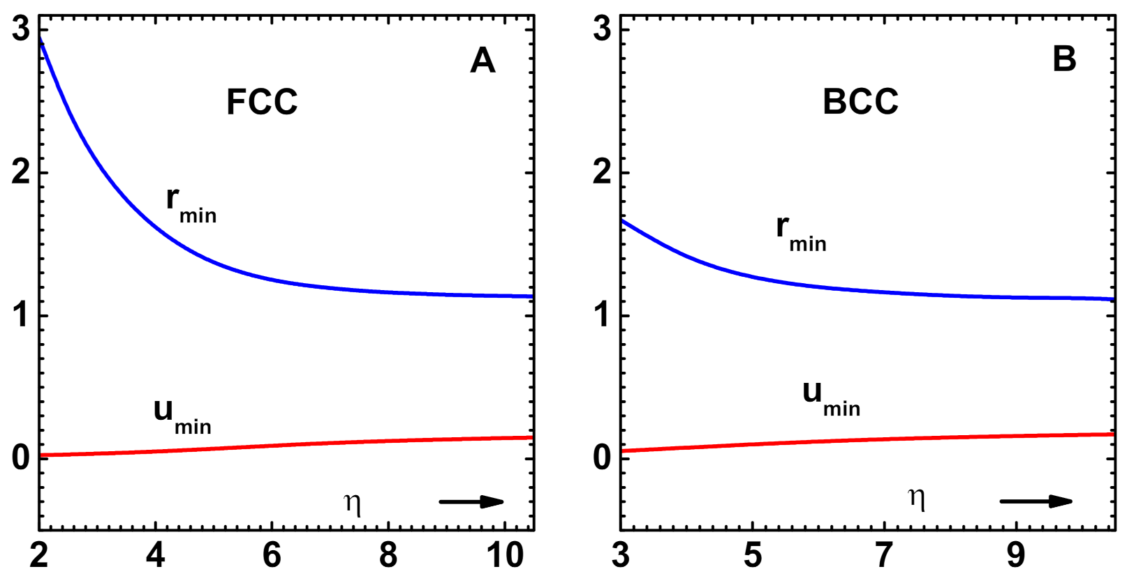
As an illustration of the model, the effective potential versus nearest-neighbor distance r for Cu (curve-1) is shown in Figure 1A. Table 6 provides the parameters used in the model. The potential minimum occurs at in reduced units. The repulsive (curve-2) and attractive (curves-3) components of the potential, as per WCA specification (see below), are also shown. The cohesive energy versus side length of atomic volume is shown in Figure 1B. Keeping all of the parameters except fixed, variations of the potential minimum and position versus are shown in Figure 2A. These results, which correspond to FCC lattices in general, show that potential parameters are somewhat insensitive to beyond . Therefore, critical point parameters, which are to be discussed below, also would show this weak dependence for larger values of . Figure 2B shows similar results, obtained using data for Fe (see Table 6), which correspond to BCC lattices. The trends of variation of the parameters are similar, although the range of variation of is much less.
Having discussed the details of obtaining the inter-particle potentials, it is now appropriate to consider a general method for computing properties of metallic fluids. Critical point parameters and phase diagrams in liquid-vapor phase transition are obtained thereafter. The scaling of cohesive energy and potential would imply such a scaling of critical point parameters with respect to and some (approximate) universal form for phase diagrams.
5. Coupling-Parameter Expansion
The CPE in thermodynamic perturbation theory [11] is based on dividing the inter-particle potential into a reference (repulsive) and perturbation (attractive) components. The most appropriate division is based on the WCA prescription [10], which is defined as
The reference part is purely repulsive and it determines the structure of dense liquids, while the attractive perturbing component is responsible for cohesion and phase changes [10]. A coupling-parameter is introduced into the potential and it is expressed as . Its magnitude determines the strength of the perturbation; with being the reference part and the full potential. All of the correlation functions, which determine the structure of the fluid, like the pair distribution function , are now to be treated as functions of . In the thermodynamic perturbation theory (TPT), these functions are expanded as Taylor’s series in regarding their reference part as
Here, is the reference system’s pair distribution function and denotes its derivatives at . Similar Taylor’s series representations hold for other correlation functions as well: the direct correlation function , the total correlation function , and the indirect correlation function . For all of them, the subscript 0 will denote the function that corresponds to the reference system. The effect of the perturbation is accurately determined if the derivatives, like , are obtained up to sufficient orders. Traditional perturbation theory is mainly limited to the first two orders [7]; however, CPE accounts for quite higher orders by taking recourse to the OZE, which defines the relation between the short ranged direct correlation function and the long ranged total correlation function . The latter is the appropriate function to be used in the OZE as it tends to zero for large r, just like the pair-potential. For one-component systems with spherically symmetric potential, as in the present case, the OZE is written as:
where is the number density of atoms. This relation has to be supplemented with a closure relation involving , and the pair-potential . An exact closure is unfeasible; however, several approximate forms are available [3]. All of the closures are generally expressed in terms of a ’bridge function’ in the form:
where , Boltzmann’s constant and T absolute temperature. Note that is also scaled with energy unit . Approximate forms of generate different closures; for instance, the one called HNC that was mentioned earlier corresponds to the choice .
Being an integral equation with displacement kernel, the OZE is easily solved in the Fourier space, leading to the solution
where the Fourier transform and its inverse, for any function , are defined as
A ’bar’ is used throughout to denote Fourier transforms. It is useful to rewrite these equations in terms of the functions and and the symmetric kernel , as discussed below.
The two algebraic equations Equations (17) and (18), although defined in two different spaces, define the non-linear systems that determine the correlation functions and entire thermodynamic properties. When the inter-particle potential contains an attractive component, solutions to the OZE with most of the closures develop singularities in the liquid-vapor transition region [14]. Hence, the determination of the critical points and phase diagrams is a difficult task, and very careful strategies need to be implemented [27]. The CPE technique completely avoids this problem of dealing with singularities, as all correlation functions are expanded in Taylor’s series. The issues that are related to convergence of the series and ’no-solution-region’ are discussed later. The Newton–Armijo non-linear solver considered next is applicable to general potentials; however, it is discussed below for the case of reference potential, as required in the CPE method.
5.1. Newton-Armijo Solver for Reference System
For repulsive inter-particle potentials, as in the case of reference system, an accurate form of bridge function [28] is , so the closure is expressed as
The solution to the OZE in terms of is given by
These nonlinear equations are readily solved while using Newton’s method [29]. While, in this reference, these are treated as two equations and two unknowns, it is possible to take Equation (20) as providing if is given. Accordingly, only Equation (21) is to be solved by Newtons’ method. Starting with initial guess solution (and, hence, , and ), an improved solution is obtained while using the first order correction terms:
where is the derivative with respect to . Taking Fourier transform of and substituting in the second equation yields
The linear operator defining this equation involves the following operations: (i) Fourier inverse taking to , (ii) multiplication by , (iii) Fourier transform of the resulting product, and (iv) multiplication by . This may be symbolically written as: , where denotes the Fourier transform. Thus, the action of essentially involves two Fourier transform operations, which is re-defined with a symmetric kernel as:
where and . Subsequently, the operator is re-defined as , where represents integration with the symmetric kernel . The adjoint of , as needed in Krylov space-based linear equation solvers discussed next, is then easily computed as .
Numerical implementation of this algorithm uses a uniformly spaced discrete coordinates with where is, typically, 10. This choice allows the use of FFT (Fast Fourier-transform) techniques. With a typical , the discrete mesh sufficiently extends to account for the asymptotic variation of the correlation functions. In Fourier space, is chosen, such that , so that orthogonality of trigonometric functions is maintained in the discrete space. With these choices, the linear equation for is reduced to a matrix equation of order , which is most efficiently solved while using Krylov space-based methods [12].
The process of improving the solution, called Newton’s iterations, is continued until the Euclidean norm is less than a prescribed value. If the norms satisfy the condition (subscripts ’1’ and ’0’ denote the current and previous iteration values, and is a small number), next Newton’s iteration follows. Otherwise, it is likely that iteration with full step would diverge. Accordingly, a smaller step size with is to be used. Note that the norms correspond to , while to . Armijo’s rule restricts the new step size to with a value of . For choosing that , a sub-iteration yielding with is performed. A quadratic fit of versus is then used to obtain , which corresponds to the minimum of in the interval . Another sub-iteration providing is performed and, if it satisfies the norm-reduction criterion, next Newton’s iteration follows. Otherwise, more sub-iterations are performed, each time with the replacements and , and, similarly, the respective norms. If the sub-iterations exceed a prescribed limit 10), it would be necessary to restart Newton’s iterations with a new guess solution.
The linear equations to be solved, at each Newton’s iteration, is of the standard form . The Conjugate Gradient (CG) method is the simplest of all iterative methods attempting a solution in the Krylov space, although it is applicable to symmetric matrices [30]. For non-symmetric matrices, as in the present case, the CG method is applicable to the normal equation as is symmetric. The algorithm starts with a guess solution and its error vector , and auxiliary vectors . Afterwards, the iteration process, called CGNR (Conjugate Gradient to Normal equations to minimize Residual) (see Appendix A), generates new solutions , such that the residual error norm is minimized at each iteration n. The process converges to the exact solution in utmost (dimension of the matrix) iterations if is non-singular [30]. In practice, iterations are terminated when the error norm satisfies a prescribed criteria. There is little point in getting a high degree of convergence in the early stages of Newton’s iterations. In what are called inexact methods, the criteria used are with a typical value . A more common method, called GMRES (Generalized Minimum Residual), although it does not need , requires much larger storage space [30].
The correlation functions of the reference system are determined with the methods discussed (also see Appendix A) in the entire fluid-phase-plane, except at very low temperatures, where perturbation theories are inapplicable.
5.2. Derivatives of Correlation Functions
The next step in CPE is to compute the derivatives, like in Equation (15). Writing the general closure relation in Equation (17) in the form , where , repeated differentiation with respect to yields
where denote the Binomial coefficients and is the Kroenecker delta. This is valid for arbitrary and, in particular, for . The arguments r and of all functions are omitted for simplifying the equations. Note that is the attractive component in the potential according to the WCA prescription. The summation in Equation (25) only contains derivatives lower than n as the term containing is separated out. Substituting for and using the relation for yields the recursion relation:
The derivative is written as , so that only contains derivatives of y of an order lower than n. This is needed, as is yet to be determined with another equation. The definition of structure factor:
shows that for . From now on, the arguments k and of all Fourier functions are also omitted. Repeated differentiation of the relation yields
where the first and last terms are separately written from the summation. Simplifying the expression and substituting in gives the recursion
Here, the definition of is used and is substituted as in the summation. Note that only contains lower order derivatives and for . Taking Fourier transform of Equation (26) and substituting in Equation (29) yields a linear equation for , which is expressed as
This expression is valid for arbitrary value of . The linear operator in this equation (for all n) is identical to that shown in Equation (23) if the derivatives are evaluated at , which is, for the reference system. Thus, the Krylov space-based methods mentioned above are also applicable here; with the only change being the source term .
5.3. Derivatives of Bridge Function
The density-dependent bridge function for a general potential with attractive component is expressed as [28]
where all are functions of r and . Defining yields for where . Now, repeated differentiation of the relation readily yields the recursion formula:
which provides all derivatives in terms of . The parameter defined earlier is now identified as , and the summation term provides .
5.4. Thermodynamic Functions
After computing the Taylor’s series for all functions to an arbitrary high order, setting provides correlation functions that correspond to the full potential. The results that are discussed below are obtained with 7th order approximation, as a further increase in order does not have any significant effect. Thermodynamic properties, like pressure and inverse compressibility , are expressed as
Similar expressions hold for internal energy and chemical potential [27]. The argument is omitted from these expressions. For computational purposes, Equation (33) is re-expressed in terms of the ’cavity function’ , as:
Here, is the second virial coefficient for U, and it is separated out explicitly. An excellent first order perturbation theory [31] for the equation of state follows from this equation with the approximations: and , thereby terminating the integral at . The second approximation is the basis of first order theory. The first approximation is motivated from the observation that derivative is only predominant near , where is small.
The OZE does not provide exact thermodynamic consistency [3] in the sense that pressure that is computed from different routes does not agree with each other. The inverse compressibility , being expressed in terms of the short ranged correlation function , is the more appropriate response function to compute pressure via integration with respect to . The method followed here employs a fine mesh of T and over the phase plane where is computed. Subsequently, two-dimensional (2-D) interpolation is used for intermediate values, and P is obtained via integration over from zero. Solutions of the critical conditions provide the critical point parameters and Maxwell’s construction the phase diagram. Using thermodynamic relations to obtain other quantities, like energy and entropy, equation of state tables [32] can be generated in the expanded volume regions.
There are some important issues underlying the above procedure. It is known that there are multiple solutions to OZE and closure relations in the two-phase region when attractive interactions are present. This is illustrated in Baxter’s analytical solution [33] of the sticky hard sphere model. These include isotherms with negative compressibility, complex, and even diverging pair distribution function. Numerical methods also show similar features for general potentials and closure relations (see following section). Solutions that are given by van der Waals equation, first order perturbation theory, and the CPE show isotherms with negative compressibility in the two-phase region. The nonphysical pressure that is generated by these approaches is replaced with a flat isotherm while using thermodynamic conditions of equal pressure and chemical potential, or the equivalent Maxwell’s construction. The use of virial pressure (Equation (33)) or inverse compressibility (Equation (34)) produces similar results via Maxwell’s construction, although some differences arise due to the inherent thermodynamic inconsistency mentioned earlier. Another approach is to compute virial pressure and chemical potential, only in regions where compressibility is positive, and then derive the phase diagram while using thermodynamic conditions [27]. The structure factor within the two-phase region is to be obtained as a weighted average of contributions of the gas and liquid phases that correspond to any point on the isotherm. Only renormalization group approaches, such as in the the hierarchical reference theory [34], generate flat isotherms in the two-phase region without using Maxwell’s construction.
Yet another relevant issue regarding the utility of Taylor’s series expansion of (and other correlation functions) needs clarification. Negative compressibility, at any phase point, implies that is negative and, by continuity requirements, would vanish at some , as it should approach unity for large k. Therefore, and, consequently, would diverge at . Thus, negative compressibility at any phase point implies a singularity in the Fourier transform (The author thanks one of the anonymous reviewers of Condensed Matter (MDPI) journal for this argument). Taylor’s series expansions that are assumed in CPE do not converge to this singular solution, in fact, numerical results indicate that they converge to a different solution (see following section). This is plausible in a scenario, wherein multiple solutions exist in the two-phase region. Their utility in computing phase diagram (via thermodynamic or Maxwell’s construction) needs to be evaluated by comparing the results with those from independent methods.
5.5. ’No-Solution-Region ’
Multiple solutions and singularities of the OZE in the liquid-vapor transition region have been investigated in detail for the Lennard-Jones (LJ) potential: , with the HNC closure [13] and other closures [14]. The pseudo-arc-length continuation algorithm is needed for the direct application of Newton’s method to the full potential for tracking these singularities [13]. The no-solution-line is defined as the curve in the phase plane, along which the Jacobian is singular and so Newton’s method is inapplicable. Figure 3A displays (curve-1) this curve for the LJ-HNC model [13].
In fact, there are more characteristic features, like the ’fold-bifurcation’ of solutions in the liquid-vapor region of the nonlinear OZE. However, the CPE method does not pick up these singularities, as it is based on series expansion about the repulsive component of the potential. The situation is similar that of van der Waals equation, although free of singularities, which predicts a region of negative compressibility. Figure 3A also shows the spinodal line ( defined by ) for the LJ-HNC model, which is obtained using 7th order CPE of this paper (curve-2).
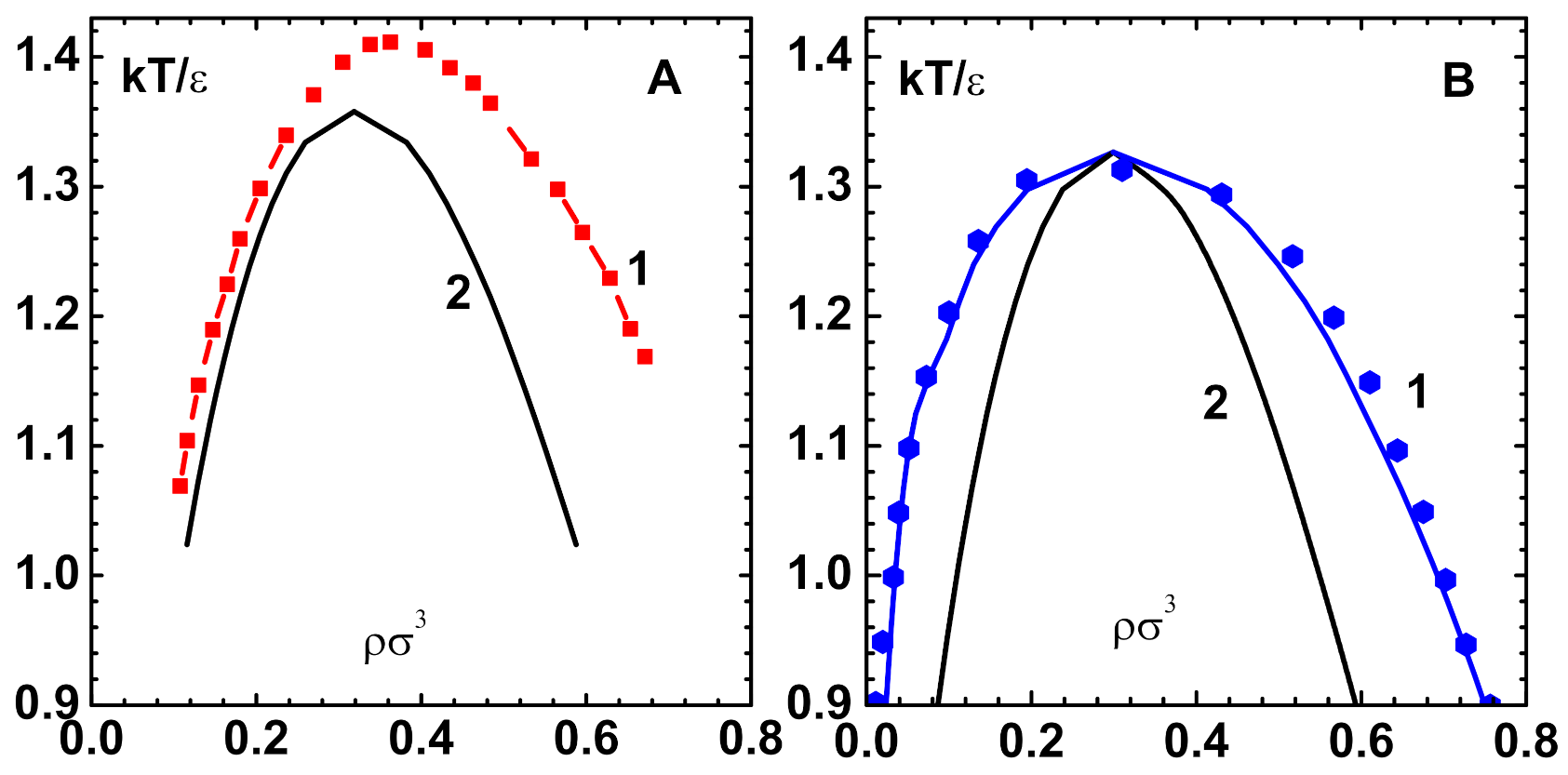
The LJ system is also investigated while using the density-dependent bridge function [28] for comparison with simulation data [35]. This is important because the bridge function is the sole ingredient that determines the predictive power of OZE. The results for phase diagram (co-existence curve) that were obtained with CPE shown (curve-1) in Figure 3B compare well with simulation data (symbols). There is only slight disagreement along the liquid branch near the transition point. The critical point parameters obtained: and also compare well with simulation data given in square brackets. The spinodal line (curve-2), which is different from that obtained with HNC, is also shown.
As discussed in the previous section, it is necessary to check wheter the CPE generates any meaningful correlation functions, particularly in the two-phase region. Figure 4A shows the direct correlation function (curve-c), the reference function (curve-0), and six successive derivative terms (curve-1 to curve-6) for the LJ system using the density-dependent bridge function [28]. These correspond to the phase point and , which is in the spinodal region. It is evident that the expansion approaches a well defined function . The reference function is mostly negative, but the positive part in for , arising out of attractive interactions, gives rise to negative compressibility. Similarly, Figure 4B shows the pair distribution function (curve-g), the reference function (curve-0), and six derivative terms (curve-1 to curve-6), also corresponding to the same phase point. The reference function with a small peak develops to with two well defined peaks due to attractive interactions. It will be more accurate to use the series expansions in Equation (17) (closure relation) for computing . These ’correlation functions’ are nonphysical, as they generate negative compressibility and van der Waals’s loop in pressure, but they may be used in order to compute phase diagram via Maxwell’s construction. Afterwards, it will be necessary to take the weighted averages (as explained earlier for structure factor) of contributions of gas and liquid phases to obtain physically acceptable correlation functions.
6. Liquid-Vapor Phase Transition in Metals
The CPE method and inter-particle potentials that are derived via lattice inversion method for metallic fluids are next evaluated as these have softer repulsive components. The simulation results using Morse potential [36] with parameters corresponding to Au and Cu are used for comparing phase diagrams. The data that are given in Table 6 and the cohesive energy formula in Equation (4) provide the parameter-free potentials for use in CPE.
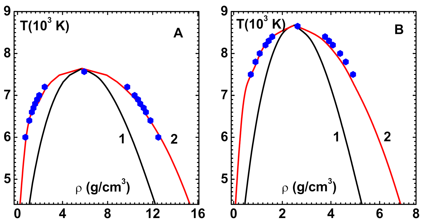
The results shown (curve-2) in Figure 5A and simulation data [36] (symbols) for Au agree quite well. Critical point parameters of CPE method, viz., g/cm , K and GPa and simulations (given in square brackets) also agree well. The spinodal curve (defined by ) is also shown (curve-1). A similar comparison of phase diagram for Cu is shown (curve-2) in Figure 5B with simulation data [36] (symbols). The critical point parameters g/cm , K and GPa also compare reasonably with the simulation results that are given in square brackets.
Scaling of Critical Parameters and Phase Diagram
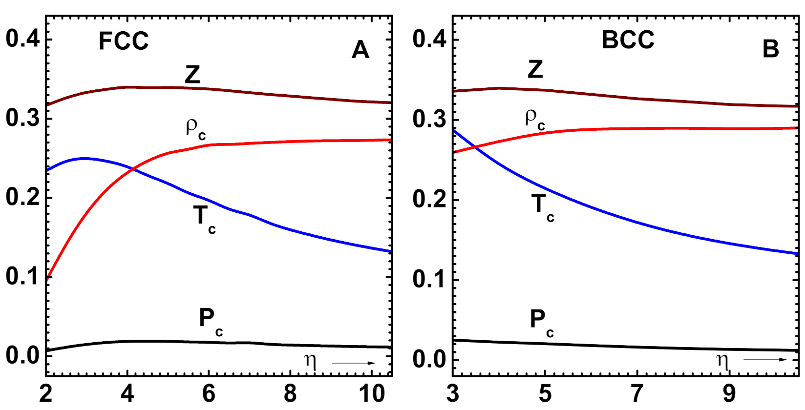
Having established the accuracy of methods, the scaling behavior of critical point parameters and phase diagram is now investigated. As the cohesive energy formula in Equation (4) only contains two parameters, ( and ), it is obvious that the effective potentials and, hence, all of the features that are related to co-existence also only depend on these variables. Of these two, is generally a small number (see Table 6). Computations utilizing CPE are performed to determine the variation of critical point parameters: and , with the scaling variable , and results for FCC lattices are shown in Figure 6A. Note that the graph displays dimensionless quantities that are expressed in the units: , and , respectively. Similar results for BCC lattices are provided in Figure 6B. The parameter is kept constant at 0.0808 for FCC and 0.0148 for BCC lattices. Varying this parameter within its range does not produce significant changes in these curves. For FCC lattices, the variation in and are more pronounced for smaller values of . These results are somewhat similar to those that were obtained earlier [5]; however, their variations and dependence on the lattice type are new.
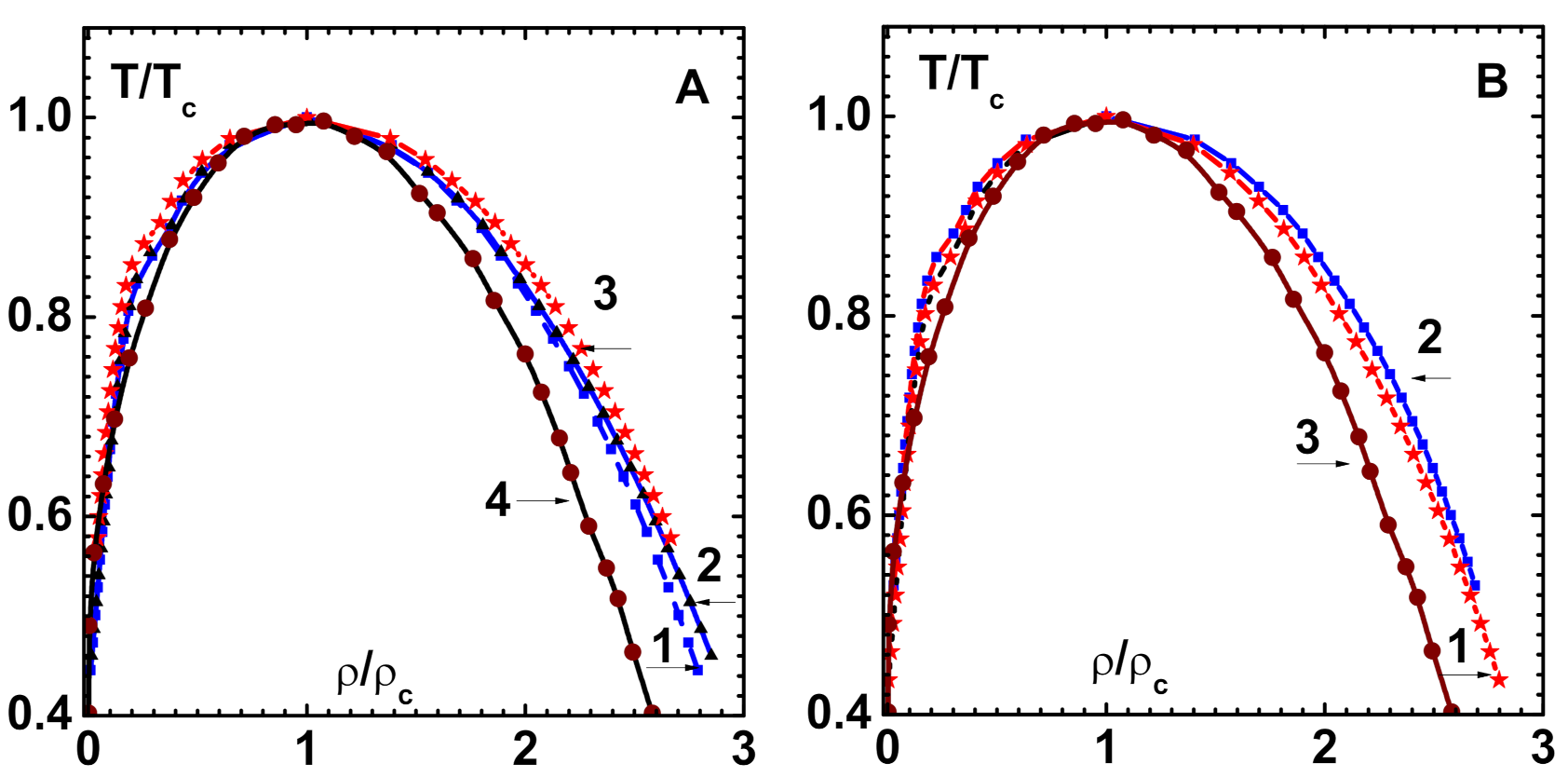
Phase diagrams for three FCC metals, Al (curve-1), Cu (curve-2), and Au (curve-3) are displayed in reduced variables and in Figure 7A. Similar results are given in Figure 7B for two BCC metals Fe(curve-1) and W(curve-2). Panels A (curve-4) and B (curve-3) also contain van der Waals phase diagram for comparison. These results indicate that there are similarities in the co-existence region for these metallic fluids, although there is no perfect universality, as in the case of van der Waals model. This is due to the fact that the interaction potentials, scaled with and , do not assume a universal form. Similar observations are also found in the simulation data of phase diagrams while using Morse potential [36].
7. Summary
The main aim in this paper is to discuss the scaling aspects of liquid–vapor phase transition in metallic fluids. There are two requirements to carry out this investigation: (i) realistic (effective) inter-particle potentials and (ii) an accurate statistical mechanical model. The four-parameter formula for cohesive energy expressed in units and consists of just two dimensionless variables ( and ). This is quite accurate in the compressed as well as expanded volume states, although it needs to be corrected for extreme compression while using the QSM for electrons. Accordingly, effective potentials derived from the cohesive energy formula will mainly depend on these variables and . Two complementary ways to impact lattice inversion are considered: (i) direct iterative method and (ii) Chen-Möbius inversion formula. New tables for inversion parameters covering up to 20 atomic shells are generated for FCC and BCC lattices, which are easily extended to other lattice types. Variations of the potential depth and first neighbor distance versus are then evaluated for the two lattices.
The statistical mechanical model using CPE is revisited and explicit recursion formulas for the derivatives of correlations and bridge function are derived. In fact, very high order derivatives are easily computed with the present formulation. The Newton–Armijo nonlinear solver together with Krylov space-based linear solvers are implemented within the CPE. The same linear solvers are applicable to solve the linear equations for the derivatives of correlation functions, as the matrices involved are the same. With these techniques, it is possible to cover the entire fluid region, except in the low temperature limit, where perturbation theory is inapplicable. The entire procedure is evaluated with simulation data for LJ system as well as metallic fluids. The ’no-solution-region’ concurring when OZE is applied to the full potential is also checked with CPE results for the LJ system. The variations of critical point parameters versus are then evaluated for FCC and BCC lattices. Further, it is also shown that the phase diagrams of these systems show (approximate) universal behavior when expressed in terms of reduced variables. It is hoped that the CPE elaborated in this paper would be increasingly used to derive thermodynamic properties of one component fluids. To that end, the Appendix A (Algorithms A1–A5) provides short outlines of the main algorithmic components.
Funding
This research received no external funding.
Acknowledgments
The author thanks the reviewers of Condensed Matter Journal
for critical reviews and suggestions to improve the presentation of the paper.
Conflicts of Interest
The author declare no conflict of interest.
Appendix A. Algorithm for CPE
The main components of the algorithm to implement CPE is provided below. Newton is the non-liner solver for the reference potential and CGNR is the linear solver. Other linear solvers, like GMRES, can also be used. Matrix computes matrix-vector products in the linear solver. Recursive equations for derivatives of correlation functions are in Derivative. The heart of the algorithm is fast Fourier transforms provided in Fourier. Note that and are the global variables used in Matrix.
| Algorithm A1: Newton |
| in: |
| out: |
| While Do |
| if Exit |
| Algorithm A2: CGNR |
| in: |
| out: |
| While Do |
| if Exit |
| Algorithm A3: Matrix |
| in: x |
| out: y |
| If (p .eq. 1) |
| If (p .eq. 2) |
| |
| Algorithm A4: Derivative [] |
| in: |
| out: |
| While Do |
| Algorithm A5: Fourier |
| in: p |
| out: y |
| Do: |
| |
| Do : |
| Do: |
| Do: |
| Do : |
| Do : |
| Do : |
| Do : |
| Do : |
| Do : |
| Do : |
References
- Landau, L.D.; Lifshitz, E.M. Statistical Physics; Pergamon Press: London, UK, 1959. [Google Scholar]
- Menon, S.V.G. Renormalization Group Theory of Critical Phenomena; Wiley Eastern Ltd.: Bengaluru, India, 1995; Available online: https://www.researchgate.net/publication/260165199 (accessed on 23 January 2021).
- Hansen, J.P.; McDonald, I.R. Theory of Simple Liquids, 4th ed.; Academic Press: Cambridge, MA, USA, 2013. [Google Scholar]
- Rose, J.H.; Smith, J.R.; Guinea, F.; Ferrante, F. Universal features of the equation of state of metals. Phys. Rev. B 1984, 29, 2963. [Google Scholar] [CrossRef]
- Rosenfeld, Y. Predicting the liquid-vapor critical point from the crystal anharmonicity. Contrib. Plasma Phys. 2001, 41, 183. [Google Scholar] [CrossRef]
- Kerley, G.I. Perturbation theory and the thermodynamic properties of fluids. II. J. Chem. Phys. 1980, 73, 478. [Google Scholar] [CrossRef]
- Solana, J.R. Perturbation Theories for Thermodynamic Properties of Fluids and Solids; CRC Press: New York, NY, USA, 2013. [Google Scholar]
- Cowen, B.J.; Carpenter, J.H. Improved reference system for corrected rigid spheres equation of state model. J. Appl. Phys. 2020, 128, 055901. [Google Scholar] [CrossRef]
- Li, J.H.; Liang, S.H.; Guo, H.B.; Liu, B.X. Four-parameter equation of state and determination of the thermal and mechanical properties of metals. J. Alloys Compd. 2007, 431, 23. [Google Scholar] [CrossRef]
- Weeks, J.D.; Chandler, D.; Andersen, H.C. Role of Repulsive Forces in Determining the Equilibrium Structure of Simple Liquids. J. Chem. Phys. 1971, 54, 5237. [Google Scholar] [CrossRef]
- Ramana, A.S.V.; Menon, S.V.G. Coupling-parameter expansion in thermodynamic perturbation theory. Phys. Rev. E 2013, 87, 022101. [Google Scholar] [CrossRef]
- Kelley, C.T. Solving Nonlinear Equations with Newton’s Method, Fundamentals of Algorithms; SIAM: Philadelphia, PA, USA, 2003. [Google Scholar]
- Peplow, A.T.; Beardmore, R.E.; Bresme, F. Algorithms for the computation of solutions of Ornstein-Zernike Equation. Phys. Rev. E 2006, 74, 046705. [Google Scholar] [CrossRef]
- Tikhonov, D.A.; Sarkisov, G.N. Singularities of solution of the Ornstein-Zernike Equation within the gas-liquid transition region. Russ. J. Phys. Chem. 2000, 74, 470. [Google Scholar]
- Gillan, M.J.; Alfe, D.; Brodholt, J.; Vocadlo, L.; Price, G.D. First-principles modeling of Earth and planetary materials at high pressure and temperatures. Rep. Prog. Phys. 2006, 69, 2365. [Google Scholar] [CrossRef]
- Kalitkin, N.N.; Kuz’mina, L.V. Curves of cold compression at high pressures. Sov. Phys. Solid State 1972, 13, 1938. [Google Scholar]
- More, R.M. Quantum-statistical model for high-density matter. Phys. Rev. A 1979, 19, 1234. [Google Scholar] [CrossRef]
- Kerley, G.I. User’s Manual for PANDA II- A Computer Code for Calculating Equation of State; Sandia Report, SAND88-229.UC-405; Sandia: Albuquerque, NM, USA, 1991. [Google Scholar]
- Heltemes, T.A.; Moses, G.A. BADGER v 1.0: A Fortran equation of state library. Comput. Phys. Commun. 2012, 183, 2629. [Google Scholar] [CrossRef]
- Carlsson, A.E.; Gelatt, C.D., Jr.; Ehrenreich, H. An ab initio pair potential applied to metals. Philos. Mag. A 1980, 41, 241. [Google Scholar] [CrossRef]
- Bazant, M.Z.; Kaxiras, E. Modeling of covalent bonding in solids by inversion of cohesive energy curves. Phys. Rev. Lett. 1996, 77, 4370. [Google Scholar] [CrossRef] [PubMed] [Green Version]
- Wiley, J.D.; Seman, J.A. The enumeration of neighbors on cubic and hexagonal-based lattices. Bell Syst. Tech. J. 1970, 49, 355. [Google Scholar] [CrossRef]
- Nan-Xian, C.; Zhao-Dou, C.; Yu-Chuan, W. Multidimensional inverse lattice problem and a uniformly sampled arithmetic Fourier transform. Phys. Rev. E 1997, 55, R5. [Google Scholar] [CrossRef] [Green Version]
- Daw, M.S.; Baskes, M.I. Embedded-atom method: Derivation and application to impurities, surfaces and other defects in metals. Phys. Rev. B 1984, 29, 6443. [Google Scholar] [CrossRef] [Green Version]
- Xie, Q.; Zhang, W.; Chen, N. Analytical long-range embedded-atom potentials. arXiv 1997, arXiv:9610183v2. [Google Scholar]
- Foiles, S.M. Application of the embedded-atom method to liquid transition metals. Phys. Rev. B 1985, 32, 3409. [Google Scholar] [CrossRef]
- Charpentier, I.; Jakse, N. Phase diagram of complex fluids using an efficient integral equation method. J. Chem. Phys. 2005, 123, 204910. [Google Scholar] [CrossRef] [PubMed]
- Sarkisov, G.N. Structure of simple fluid in the vicinity of the critical point: Approximate integral equation theory of liquids. J. Chem. Phys. 2003, 119, 373. [Google Scholar] [CrossRef]
- Zerah, G. An efficient Newton’s method for numerical solution of fluid integral equations. J. Comput. Phys. 1985, 61, 280. [Google Scholar] [CrossRef]
- Kelley, C.T. Iterative Methods for Solving Linear and Nonlinear Equations; SIAM: Philadelphia, PA, USA, 1995. [Google Scholar]
- Song, Y.; Mason, E.A. Statistical-mechanical theory of a new analytical equation of state. J. Chem. Phys. 1989, 91, 7840. [Google Scholar] [CrossRef]
- Menon, S.V.G.; Nayak, B. An equation of state for metals at high temperature and pressure in compressed and expanded volume regions. Condens. Matter 2019, 4, 71. [Google Scholar] [CrossRef] [Green Version]
- Baxter, R.J. Percus-Yevick equation of hard spheres with surface adhesion. J. Chem. Phys. 1968, 49, 2770. [Google Scholar] [CrossRef]
- Parola, A.; Pini, D.; Reatto, L. The smooth cut-off hierarchical reference theory of fluids. Mol. Phys. 2009, 107, 503. [Google Scholar] [CrossRef] [Green Version]
- Johnson, J.K.; Zollweg, J.A.; Gubbins, K.E. The Lennard-Jones equation of state revisited. Mol. Phys. 1993, 78, 591. [Google Scholar] [CrossRef]
- Singh, J.K.; Adhikari, J.; Kwak, S.K. Vapor-liquid phase co-existence curves for Morse fluids. Fluid Phase Equilib. 2006, 248, 1. [Google Scholar] [CrossRef]
Figure 1.
(A) Effective potential for Cu versus scaled nearest-neighbor distance (curve-1, with repulsive (curve-2) and attractive components (curve-3) as per WCA prescription. Potential minimum is at in reduced units. (B) Cohesive energy for Cu versus scaled side length of atomic volume x. Energy minimum () occurs at (1) in reduced units. Length and energy units are and (see text), respectively.

Figure 2.
(A) Potential minimum and its position versus for FCC lattices. All other parameters correspond to those of Cu (see text). (B) Similar results for BCC lattices. All of the parameters, except , correspond to those of Fe (see text).
Figure 2.
(A) Potential minimum and its position versus for FCC lattices. All other parameters correspond to those of Cu (see text). (B) Similar results for BCC lattices. All of the parameters, except , correspond to those of Fe (see text).

Figure 3.
(A) The ’no-solution-line’ (curve-1) for Lennard–Jones potential and hypernetted chain (HNC) obtained with pseudo-arc-length continuation algorithm [13]. Newton’s method applied to the full potential diverges on this curve. The spinodal line (curve-2) (defined by ) obtained using the CPE of this paper lies inside the no-solution region. (B) Comparison of co-existence line (curve-1), obtained with CPE and density-dependent bridge function [28], with simulation results (symbols) [35]. The spinodal line (curve-2), which is different from that obtained with HNC, is also shown.

Figure 4.
Convergence of coupling-parameter expansion (CPE) for the direct correlation function and pair distribution function for the LJ system (obtained with density-dependent bridge function [28]) at the phase point and , which is in the spinodal region. (A) Direct correlation function (curve-c), reference function (curve-0) and successive derivative terms (curve-1 to curve-6) are shown. (B) Pair distribution function (curve-g), reference function (curve-0) and derivative terms (curve-1 to curve-6) are shown.

Figure 5.
Comparison of phase diagram obtained with 7th order CPE and density-dependent bridge function [28] against simulation data for soft repulsive potentials occurring in metallic fluids: (A) The CPE phase diagram for Au (curve-2) and simulation results (symbols) using Morse potential [36] (see text). The spinodal curve (defined by ) that shows the boundary of meta-stable states (curve-1) is also shown. (B) The CPE phase diagram for Cu (curve-2) is compared against simulation results (symbols) using Morse potential [36] (see text). The spinodal curve (curve-1) is also shown.

Figure 6.
Variation of critical point parameters: , and , with the scaling variable (see text). Note that these quantities are expressed in the units: , and , respectively. (A) The results for FCC lattices. (B) Results for BCC lattices.
Figure 6.
Variation of critical point parameters: , and , with the scaling variable (see text). Note that these quantities are expressed in the units: , and , respectively. (A) The results for FCC lattices. (B) Results for BCC lattices.

Figure 7.
Phase diagram of metals in reduced variables and . (A) FCC metals Al (curve-1), Cu (curve-2) and Au (curve-3). van der Waals phase diagram is also shown (curve-4). (B) Similar results for BCC metals Fe (curve-1) and W (curve-2). van der Waals phase diagram is shown (curve-3) for comparison.


Table 1.
Shell radii and occupation numbers for FCC lattice. (see Equation (6)).
Table 1.
Shell radii and occupation numbers for FCC lattice. (see Equation (6)).
| n | n | n | n | ||||||||
|---|---|---|---|---|---|---|---|---|---|---|---|
| 1 | 12 | 1 | 6 | 8 | 11 | 24 | 16 | 48 | |||
| 2 | 6 | 7 | 48 | 12 | 24 | 17 | 30 | ||||
| 3 | 24 | 8 | 6 | 13 | 72 | 18 | 72 | ||||
| 4 | 12 | 2 | 9 | 36 | 3 | 14 | 48 | 19 | 24 | ||
| 5 | 24 | 10 | 24 | 15 | 12 | 4 | 20 | 48 |
Note that . There is no shell of radius .
Table 2.
Shell radii and occupation numbers for BCC lattice. (see Equation (6))
Table 2.
Shell radii and occupation numbers for BCC lattice. (see Equation (6))
| n | n | n | n | ||||||||
|---|---|---|---|---|---|---|---|---|---|---|---|
| 1 | 8 | 1 | 6 | 6 | 11 | 12 | 16 | 24 | |||
| 2 | 6 | 7 | 24 | 12 | 48 | 17 | 8 | 4 | |||
| 3 | 12 | 8 | 24 | 13 | 30 | 18 | 48 | ||||
| 4 | 24 | 9 | 24 | 14 | 24 | 19 | 24 | ||||
| 5 | 8 | 2 | 10 | 32 | 3 | 15 | 24 | 20 | 48 |
Note that there is no formula for radii in BCC lattice.
Table 3.
Constants of Chen–Möbius inversion formula for FCC lattice.
| n | n | n | n | ||||||||||||
|---|---|---|---|---|---|---|---|---|---|---|---|---|---|---|---|
| 1 | 12 | 1/12 | 6 | 8 | 1/9 | 11 | 24 | 16 | 24 | ||||||
| 2 | 6 | 7 | 48 | 12 | 24 | 7/72 | 17 | 24 | |||||||
| 3 | 24 | 8 | 6 | 1/32 | 13 | 72 | 18 | 24 | |||||||
| 4 | 12 | 9 | 36 | 1/12 | 14 | 0 | 1/3 | 19 | 24 | ||||||
| 5 | 24 | 10 | 24 | 0 | 15 | 48 | 1/3 | 20 | 24 | 5/24 |
Note that and are introduced.
Table 4.
Constants of Chen–Möbius inversion formula for BCC lattice.
| n | n | n | |||||||||
|---|---|---|---|---|---|---|---|---|---|---|---|
| 1 | 8 | 1 | 0.12500 | 6 | 0 | 0.03955 | 11 | 0 | |||
| 2 | 6 | 7 | 0 | 0.28125 | 12 | 0 | 0.5625 | ||||
| 3 | 0 | 0.07031 | 8 | 24 | 13 | 6 | 0.09375 | ||||
| 4 | 0 | 9 | 8 | 14 | 0 | 0.02225 | |||||
| 5 | 12 | 10 | 0 | 15 | 0 | 0.31641 |
Note that and , and many others are introduced.
Table 5.
Constants of Chen–Möbius inversion formula for BCC lattice—continued.
| n | n | n | |||||||||
|---|---|---|---|---|---|---|---|---|---|---|---|
| 16 | 24 | 21 | 24 | 26 | 32 | ||||||
| 17 | 0 | 22 | 0 | 27 | 0 | ||||||
| 18 | 24 | 23 | 0 | 0.5625 | 28 | 0 | 0.01251 | ||||
| 19 | 0 | 0.21094 | 24 | 0 | 0.63281 | 29 | 12 | 0.75 | |||
| 20 | 0 | 25 | 0 | 0.5625 | 30 | 0 | 0.26697 |
Note that and , and many others are new.
Table 6.
Material Parameters for four-parameter model .
| Material | At. No. | At. Wt. | |||||||
|---|---|---|---|---|---|---|---|---|---|
| GPa | eV | A | |||||||
| Copper | 11.38 | 134.8 | 5.19 | 3.489 | 5.0619 | 0.0808 | 2.2771 | 29 | 63.50 |
| Aluminum | 16.35 | 79.3 | 4.37 | 3.389 | 4.6361 | 0.0296 | 2.5382 | 13 | 26.98 |
| Gold | 16.95 | 180.7 | 5.43 | 3.812 | 6.7182 | 2.5686 | 79 | 196.97 | |
| Iron | 11.81 | 163.0 | 4.50 | 4.281 | 5.0270 | 0.0148 | 2.2775 | 26 | 55.85 |
| Tungsten | 15.82 | 325.0 | 4.36 | 8.791 | 5.732 | 2.2775 | 74 | 183.85 |
Publisher’s Note: MDPI stays neutral with regard to jurisdictional claims in published maps and institutional affiliations. |
© 2021 by the author. Licensee MDPI, Basel, Switzerland. This article is an open access article distributed under the terms and conditions of the Creative Commons Attribution (CC BY) license (http://creativecommons.org/licenses/by/4.0/).
Share and Cite
MDPI and ACS Style
Menon, S.V.G. Scaling of Phase Diagram and Critical Point Parameters in Liquid-Vapour Phase Transition of Metallic Fluids. Condens. Matter 2021, 6, 6. https://0-doi-org.brum.beds.ac.uk/10.3390/condmat6010006
AMA Style
Menon SVG. Scaling of Phase Diagram and Critical Point Parameters in Liquid-Vapour Phase Transition of Metallic Fluids. Condensed Matter. 2021; 6(1):6. https://0-doi-org.brum.beds.ac.uk/10.3390/condmat6010006
Chicago/Turabian StyleMenon, S.V.G. 2021. "Scaling of Phase Diagram and Critical Point Parameters in Liquid-Vapour Phase Transition of Metallic Fluids" Condensed Matter 6, no. 1: 6. https://0-doi-org.brum.beds.ac.uk/10.3390/condmat6010006