
Study of Light Polarization by Ferrofluid Film Using Jones Calculus


1
Soft Matter Lab, School of Arts, Sciences and Humanities, University of São Paulo, Sao Paulo 03828-000, Brazil
2
Space Science Center, 235 Martindale Drive, Morehead State University, Morehead, KY 40531, USA
*
Author to whom correspondence should be addressed.
Condens. Matter 2022, 7(1), 28; https://0-doi-org.brum.beds.ac.uk/10.3390/condmat7010028
Submission received: 13 February 2022
/
Revised: 5 March 2022
/
Accepted: 7 March 2022
/
Published: 9 March 2022
Abstract
:We studied the polarized light patterns obtained using a thin film of ferrofluid subjected to an applied magnetic field. We obtained patterns of polarized light with magnetic field configurations between parallel plates, monopolar, tetrapolar, and hexapolar, and studied how polarized light varies for different intensities and orientations of the applied magnetic field. Using the Jones calculus, we explored the key optical properties of this system and how these properties relate to the applied magnetic field. We have observed general aspects of polarized light obtained by transmission in a Ferrocell using polariscopes and analyzing the resulting Jones vector, such as the formation and rotation of dark bands known as isogyres. We suggest that in a thin film of ferrofluid as in a Ferrocell, two effects occur. The primary effect is dichroism, which is more sensitive to the component of the magnetic field in the direction parallel to the film plane. The secondary effect is the birefringence that can be observed by analyzing the circular polarization of light. Birefringence is related to the thin film thickness of ferrofluid.
1. Introduction
There are certain things that lead us to think about nature. Humanity is in contact with luminous patterns in nature that have aroused our curiosity since antiquity. Take, for example, rainbows, halos, glories, and other atmospheric phenomena that are present in our daily lives. Besides the contemplative aspect of these phenomena, we also have the practical results of these luminous effects. For example, some of the development of mathematical physics techniques used in engineering and science today were created by scientists who fundamentally studied rainbows, or the serendipitous case of C. R. T. Wilson, who attempted to reproduce in the laboratory the Glory effect by the development of the device known as “the cloud chamber”, which is now used to observe the presence of cosmic rays, earning him the Nobel prize for Physics in 1927 [1]. Besides pattern formation, the effects of magnetism have motivated the study of the universe. For example, when Albert Einstein was a child, his father gave him a compass. Many years later, Einstein reported that this first contact with the compass motivated him to understand different aspects of physics because “something deeper had to be hidden behind things”, such as observing the movement of the compass needle, always pointing in the same direction, no matter which way he turned the compass, made such an impact on him. The connection between electricity and magnetism is described today by Einstein’s special theory of relativity [2].
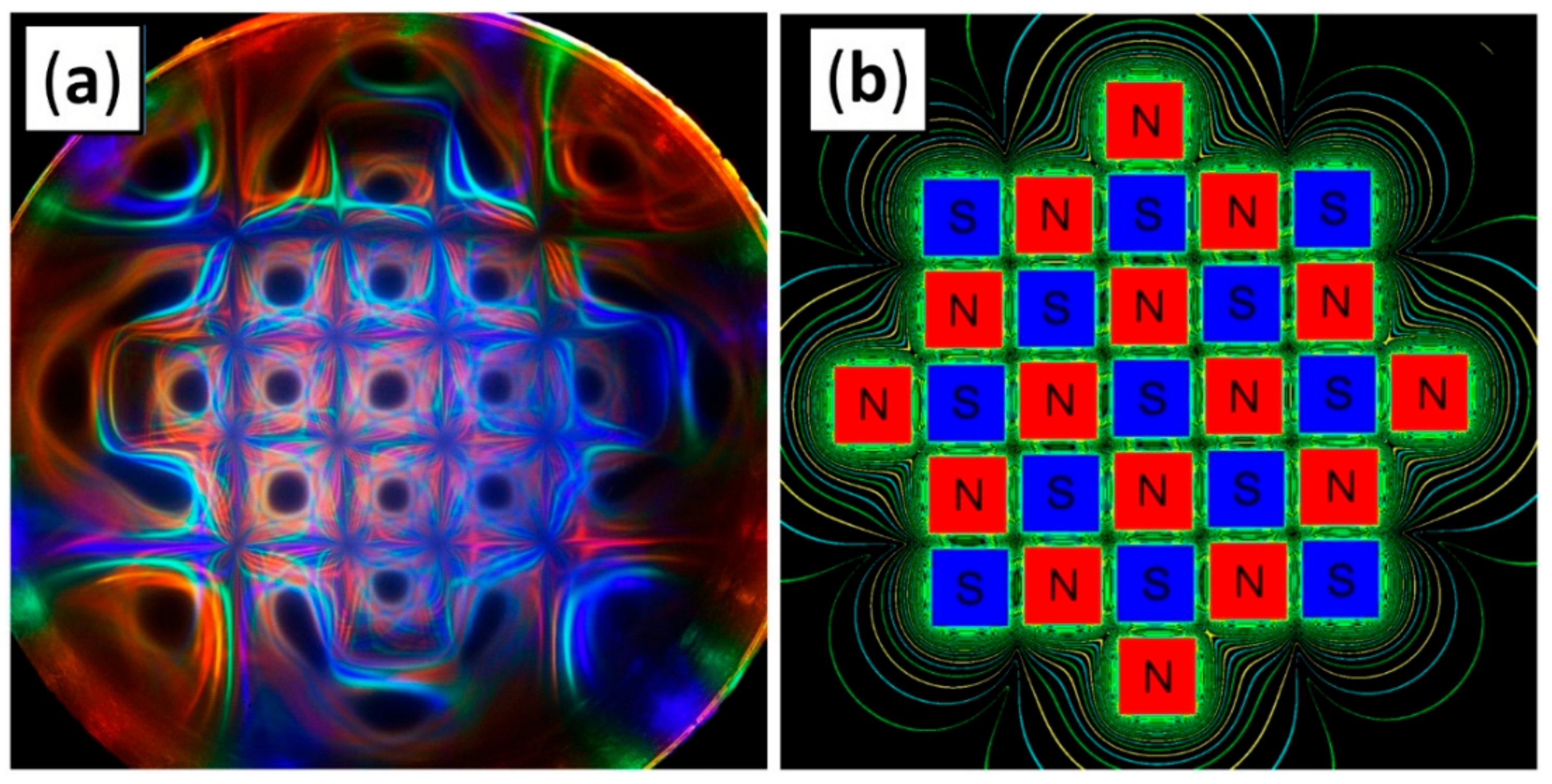
Certain phenomena that simultaneously involve optics and magnetism are known as magneto-optical phenomena and can be observed with a device known as Ferrocell, in which one can see several interesting effects, such as Horocycles of light [3] or light polarization [4,5,6,7,8]. Left and right polarization of light can propagate at different speeds in ferrofluids leading to birefringence and dichroism and making possible some technological applications such as tunable gratings, optical modulators, and sensors [4,5,6,7,8,9,10,11,12,13,14,15,16,17], which explains the increased interest in understanding the features behind this system in matters such as the polarization of light [18,19,20,21]. In Figure 1, we show the image of light that propagated through a ferrofluid that was altered by the presence of a magnetic field in a device known as a Ferrocell. The lines of light in this kind of set-up are mostly perpendicular to the magnetic field [22,23].
Some authors suggested that studies involving situations of transverse configuration in ferrofluids are important for understanding some magneto-optical properties [18]. The transverse configuration is related to the component of the magnetic field perpendicular to the direction of propagation of light. As Ferrocell is a thin film of ferrofluid, this system is ideal for studying the effects of light in ferrofluid in a transverse configuration, directly observing the light patterns, and facilitating understanding of how light is scattered by magnetic nanoparticles aligned with a magnetic field.
During our explorations with the polarized light in the Ferrocell, we observed evidence of the coexistence of effects in linear polarized light and in circular polarized light, which made us question what are the causes that can create such a phenomenon? In the literature, we can find some methods to explore and find answers for this question [24,25,26].
For this reason, the present work is based on our previous works that studied the polarization of light in ferrofluid thin films with the Ferrocell [20], and now we present an interpretation of the results we obtained using polariscopes with a formal representation of the Jones calculus, Stokes parameters, and Poincaré sphere. As far as we know, this work presents for the very first time a connection between polariscopic experiments and Ferrocell, with the observation of patterns involving structures known as isogyres and their relationship with the orientation of magnetic field lines, which in turn has a direct consequence in the study of ferrofluid magneto-optics. These results can be used to study the light patterns with the different effects that can occur in the scattering of light by nanoparticles under the effect of magnetic fields.
2. Materials and Methods
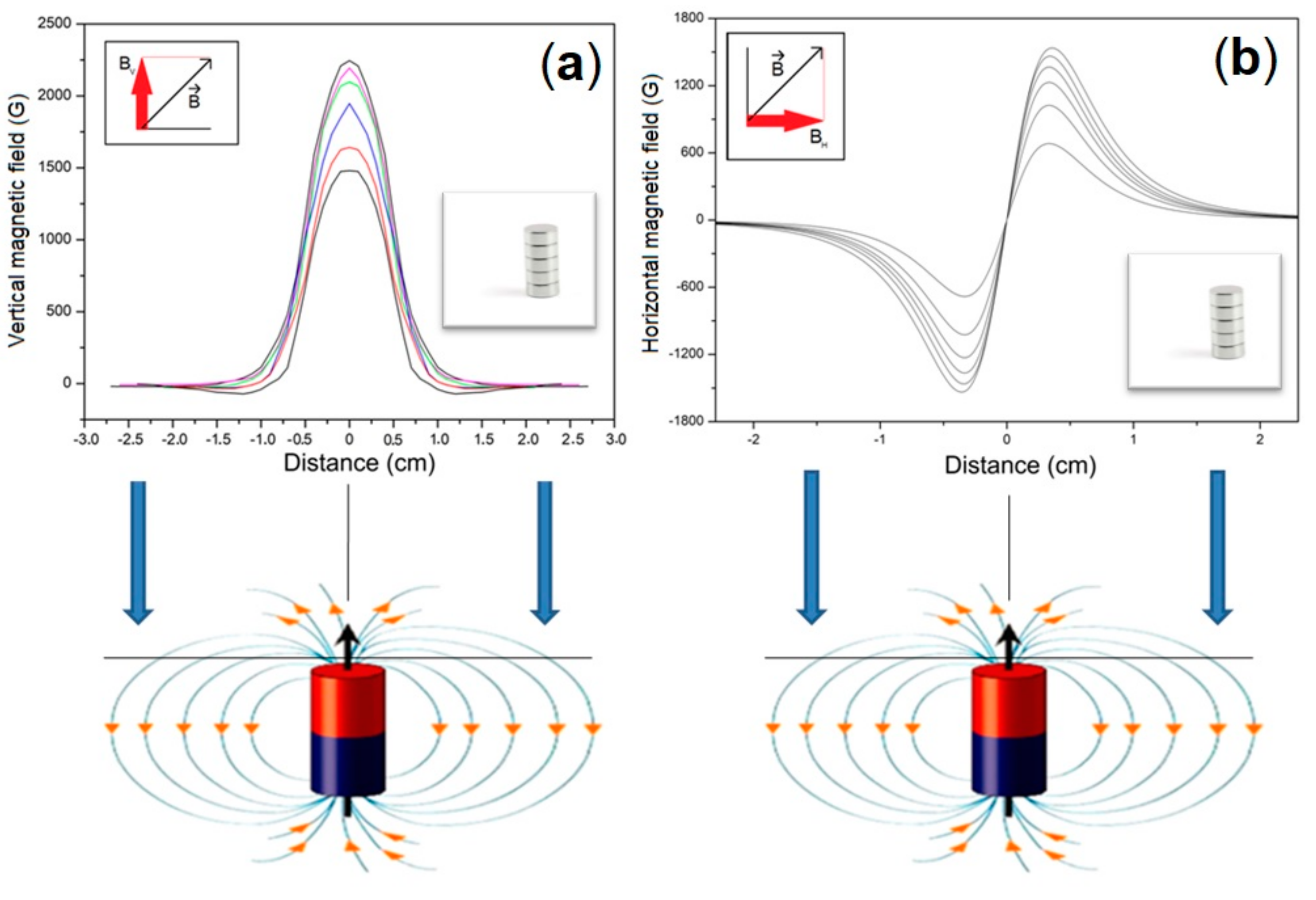
In this work, permanent magnets were used as sources of a magnetic field in the Ferrocell, whose ferrofluid film defines a plane. Thus, we need to know the orientation of the magnetic field in this plane. For example, in Figure 2, we show the vertical and horizontal magnetic field components in the Ferrocell plane for a column of cylindrical magnets.
The magnetic field is obtained by placing a cylindrical magnet over the Ferrocell. To increase the magnetic field strength, we placed other identical magnets on the first magnet, which provided the field increase, allowing the use of the magnetic field strength as an independent variable in this system. The field components were measured from the central point on one of the faces of the magnetic cylinder and moved linearly from this point with a Hall sensor on the surface of the plane where the Ferrocell will be placed.
This is the field configuration called monopolar, as the Ferrocell was exposed mainly to one of the “charges” of a magnetic dipole. These rare-earth magnets allow us to easily obtain magnetic fields in the order of 0.1 T (1000 G).
In Figure 2 the different curves in each graph show the intensity of each component of the magnetic field in space as we increased the field, obtained experimentally using a gaussmeter.
We have used a thin film of ferrofluid between 2 microscope glass slides. The ferrofluid used in our experiment was the EFH1 (Ferrotec) with saturation magnetization of 440 G, with 10 nm single size domain iron oxide nanoparticles. The ferrofluid solution was placed between 2 microscope glass slides. The microscope slides used were flat pieces of glass, typically 75 by 26 mm and about 1 mm thick for the base glued to a square coverslip at the top, with each glass plate having a thickness variation of around 1 µm, forming a thin film of ferrofluid with a thickness of around 10 µm.
The ferrofluid sample was placed in the Ferrocell and sealed over 2 years ago. The magnetic field was applied, and measurements were made over a time period of 10 s of minutes to 1 h. After that, the intense magnetic field was removed. The process was repeated routinely over the past 2 years, and the results were the same. We were careful to avoid leaving the magnet directly on the Ferrocell for periods of several hours in a row, as this can cause damage to the Ferrocell, what we call Ferrocell “burning”, which occurs by the action of the magnetic field compressing the nanoparticles against each other, as well as against the glass plates, precipitating clumps of material near the magnet. When this burning happens, we simply leave the Ferrocell without the presence of a strong magnetic field for a few days, and the Ferrocell will fully recover. If the exposure of Ferrocell was longer than several hours, this can cause the destruction of the surfactant layer that surrounds the iron monodomains, permanently destabilizing the material and forming clumps of iron that do not dissolve, damaging the Ferrocell.
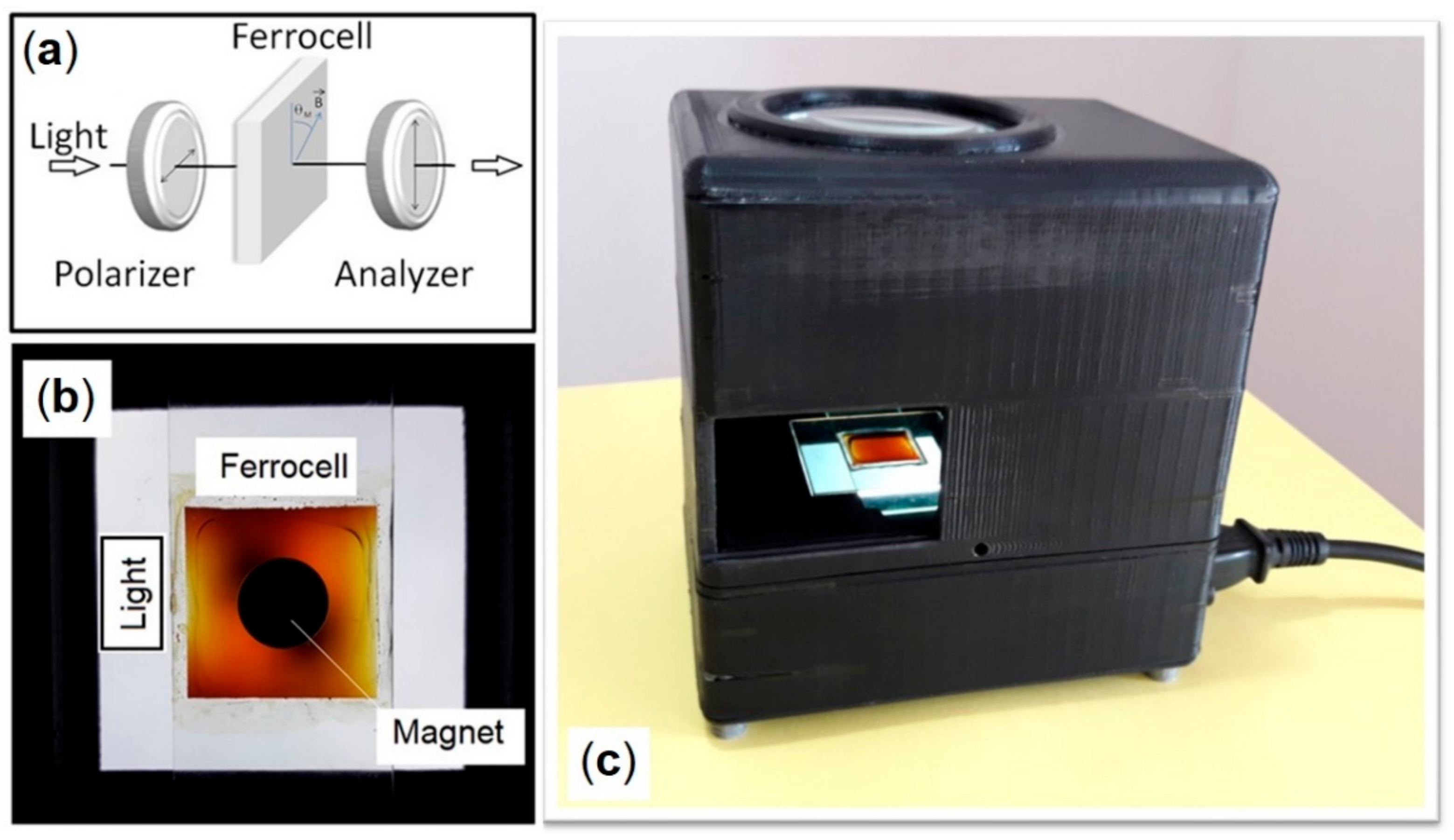
In this experiment, shown in Figure 3, we used some types of polariscopes, in which the polarization of light was used as a sensor. Thus that incident light with well-characterized polarization properties interacted with the sample. Emerging light was analyzed to understand the effects of the magnetic field in ferrofluid nanoparticles, with light following a transmission geometry. As we used linear or circular polarized light sources for different magnetic field configurations, in the next sections, we will specify which polarizer and analyzer set was being used for each respective magnetic field.
The initial light source was white, passing through a diffuser. Then the light passed through a polarizer thus that we have a plane wave illuminating the entire area of the Ferrocell with a defined polarization at each point, after which the light passed through the Ferrocell. The transmitted light passed through the analyzer polarizer. The images were recorded in a camera and transferred to a computer, where they were processed to obtain the respective light intensities.
A way of modeling the measurement of light scattering by the ferrofluid was by classical electromagnetic theory [25,27]. The basic idea was to interpret images obtained with the polariscope, as there were 4 fundamental properties of electromagnetic waves that can be explored: amplitude, phase, frequency, and polarization because a parallel beam of light interacting with a collection of particles causes several distinct effects such as absorption, elastic scattering, extinction, dichroism, and thermal emission.
Most photometric and polarimetric optical instruments measure quantities that are averages of real-valued linear combinations of products of field vector components and have dimension as intensities, such as the stokes parameters, which can be obtained considering a plane electromagnetic wave propagating in a medium with real constants ε, μ and k (permittivity, permeability, and wave number). The electric field of the light [27,28] in the position r and at instant t is given by
Ec(r,t) = E0exp(ik n.r − i ω t),
In a coordinate system used to describe the direction of propagation and the state of a plane electromagnetic wave with a couple of angles (θ, ϕ) where 0 < θ < π is the polar angle measured from the positive z-axis and 0 < ϕ < 2π is the azimuth angle measured from positive x-axis in the clockwise direction when looking in the direction of the positive z-axis. The electric field of the light at the observation point is given by
where Eθ and Eϕ are the components for the angles θ and ϕ of the electric field vector, respectively.
E = Eθ + Eϕ,
The first parameter I describes the intensity, while the Stokes parameters Q, U, and V describe the polarization of the wave. For the case of the Ferrocell, the polarization characteristics are related to mean values of size, shape, and spatial distance of the particles filling the thin film influenced by the applied magnetic field. The traditional way of studying the effects of polarization is through polarimetry, commonly used from the study of stress in materials to chirality in liquids. Therefore, it is important that we understand the Malus’ law [29] in associating polarizers and samples given by:
where I is the intensity of light and θM is the angle between each polarizer, which is a way to study the dichroism.
Since we will explore some experiments using the Ferrocell using different arrangements of optical elements, we will also use the representation of polarized light based on the Jones vectors, and Jones Matrices for the optical elements, which complements that of Stokes parameters. For example, for the case of a polarized light incident beam represented by its Jones vector Ei, in Cartesian coordinates, which passes through an optical element represented by the transformation matrix A, emerging as a new vector Et [3,29]:
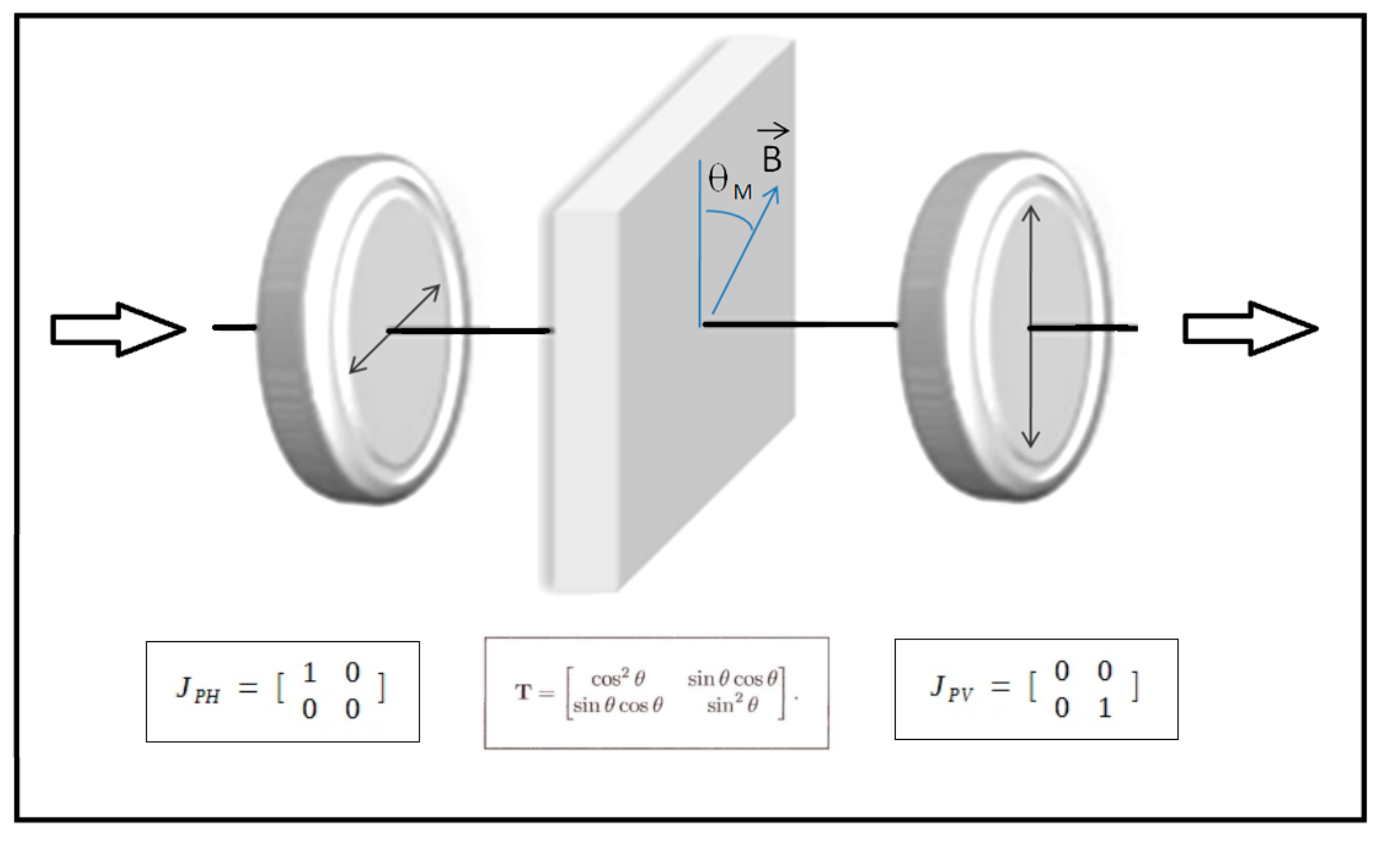
In this work, an application of the Jones Matrix calculus was to determine the intensity of output light beam when the Ferrocell subjected to a monopolar magnetic field was placed between 2 crossed polarizers. To model the effect of many media on light’s polarization state, we used Jones matrices and the related transfer function. For example, the Jones vector for the output beam is Et = J. Ei and the Jones matrix for this configuration is
3. Linear Polarization Characteristics of Light in a Ferrocell
We start showing the case when the important magnetic field component is in the plane of the film between two plates, as one can see in Figure 4. This system is equivalent to the case of the three polarizers system, in which the Malus law is commonly used. In our polariscopic experiment, when the magnetic field is aligned with the polarization axis of the first polarizer or aligned with the analyzer, the light intensity is at a minimum, while in the case in which the magnetic field lines rotated at an angle of 45° with respect to the vertical polarizer, gives the maximum light intensity. This effect is shown in Figure 5.
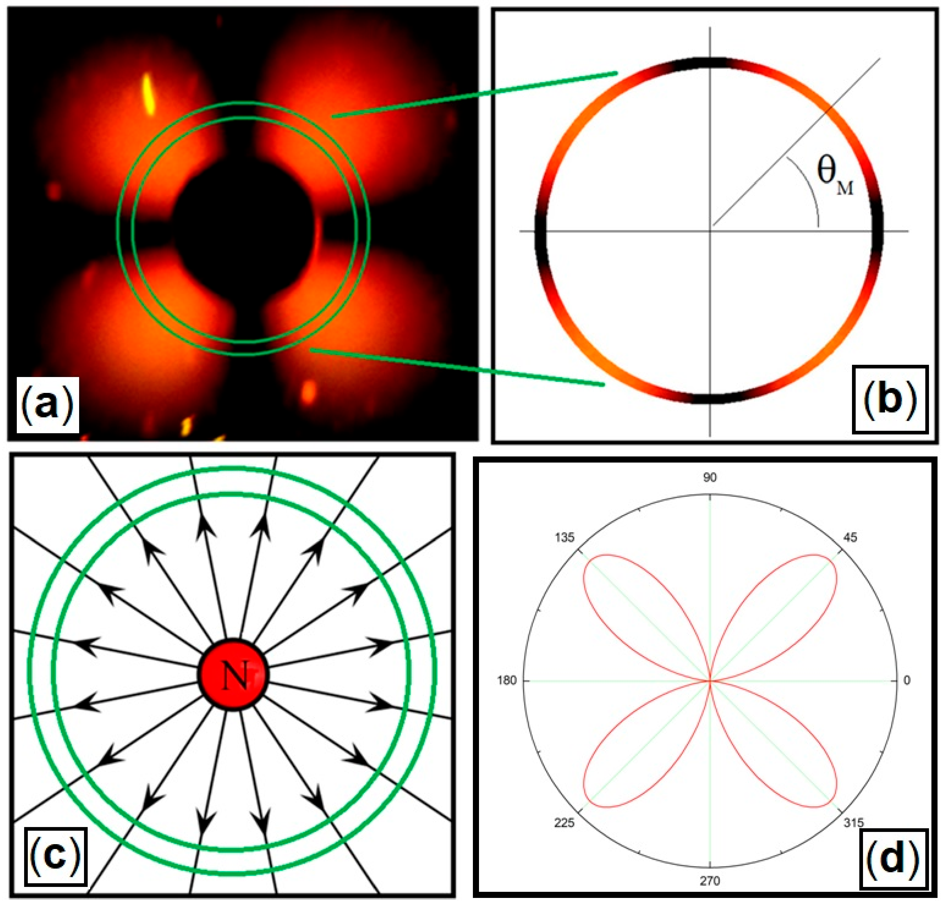
Placing a cylindrical magnet over the center of the Ferrocell in the crossed polarizer and analyzer configuration, we have the formation of a pattern that resembles a Maltese cross, as shown in Figure 6. A possible explanation for this pattern was presented in our previous works [3,20], in which we considered the absorption of polarized light by radially structures arranged within the ferrofluid due to the monopolar magnetic field. The arms of this Maltese cross form dark regions that are known asisogyres, and they occur since they show regions of cross-polarization that cut off the passage of light [20,22]. The presence of the applied magnetic field forms microneedles formed in the ferrofluid. These microneedles align in the direction of the magnetic field lines.
We can analyze the effect of absorption of polarized light considering a ring around the center of Figure 6a demarcated by the two green circles experimentally in Figure 6b and compare it with a model of a radial diffraction grating that is associated with the monopolar field of Figure 6c. For a model radial diffraction grating, the intensity in polar coordinates is shown in Figure 6d.
Applying the Malus law directly, after the first polarizer, we have a vertical linear polarized light with intensity I1, after the Ferrocell in a monopolar configuration creates a radial diffraction grating related to the diagram of the magnetic field of Figure 6c, for an angle θM in the profile of Figure 6b, the light intensity in polar coordinates after the analyzer is the image of Figure 6d forming a cross with four luminous lobes, in which the arms of the cross are isogyres. The expression for light intensity is obtained considering:
Taking into account that cos(90° − θM) = sin(θM) and sin(2θM) = 2sin(θM)cos(θM), we can reduce Equation (7) to the following expression:
We compare the plot of Equation (8) with the data obtained with the experiment in Figure 7, in which there is an agreement for the maximum and minimum values of light intensity.
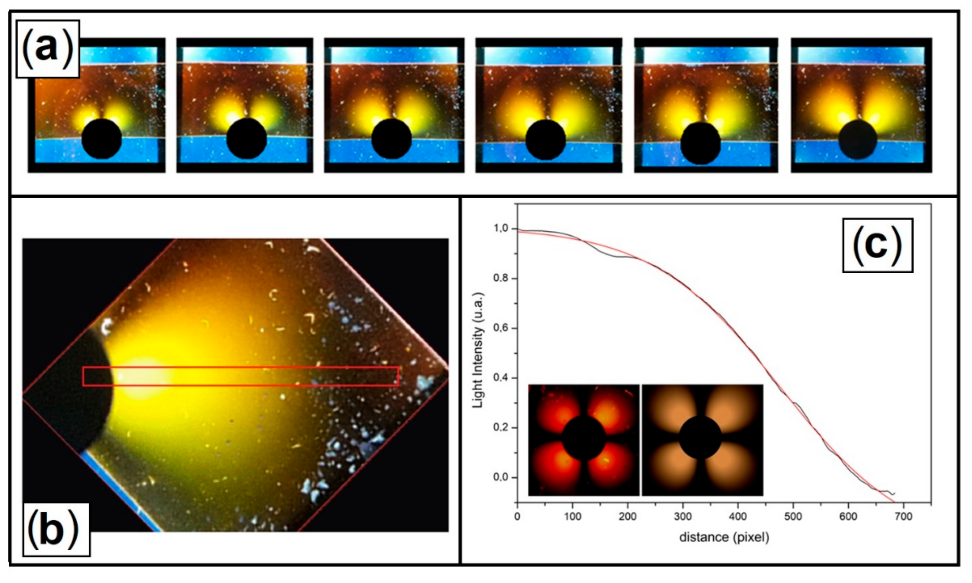
We then decided to quantitatively verify the relationship between the formation of these patterns and the intensity of the magnetic field, varying the field (Figure 8a) and observing the pattern of greater intensity that is in the equidistant line of two adjacent arms of the Maltese cross, as shown inside the rectangle red in Figure 8b. In each light pattern, the intensity decays exponentially, as in the example of Figure 8c. We have a comparison between the initial luminous pattern of Figure 6a and a simulation of this pattern inside Figure 8c using our previous work [20,30] to model polarized light in a Ferrocell.
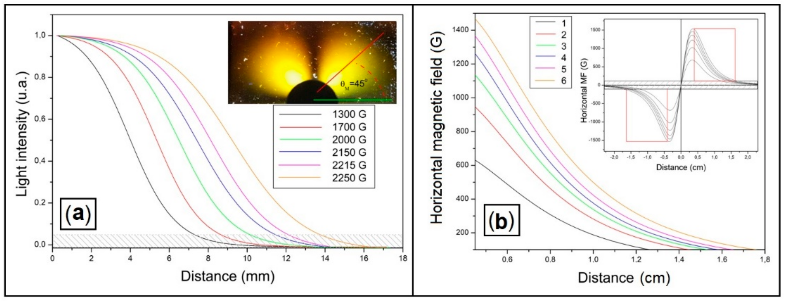
In Figure 9a, we see the graphs of the exponential decay of luminous intensity of each pattern shown in Figure 8a and Figure 9a, the variation of the horizontal magnetic field of each monopolar configuration used.
Even with the increase of the magnetic field, the light intensity is saturated and goes down exponentially in each case of the pattern of Figure 8a. We can see a strong correlation between these two graphs, which indicates that the horizontal component of the magnetic field is the most important factor in the formation of these luminous lobes.
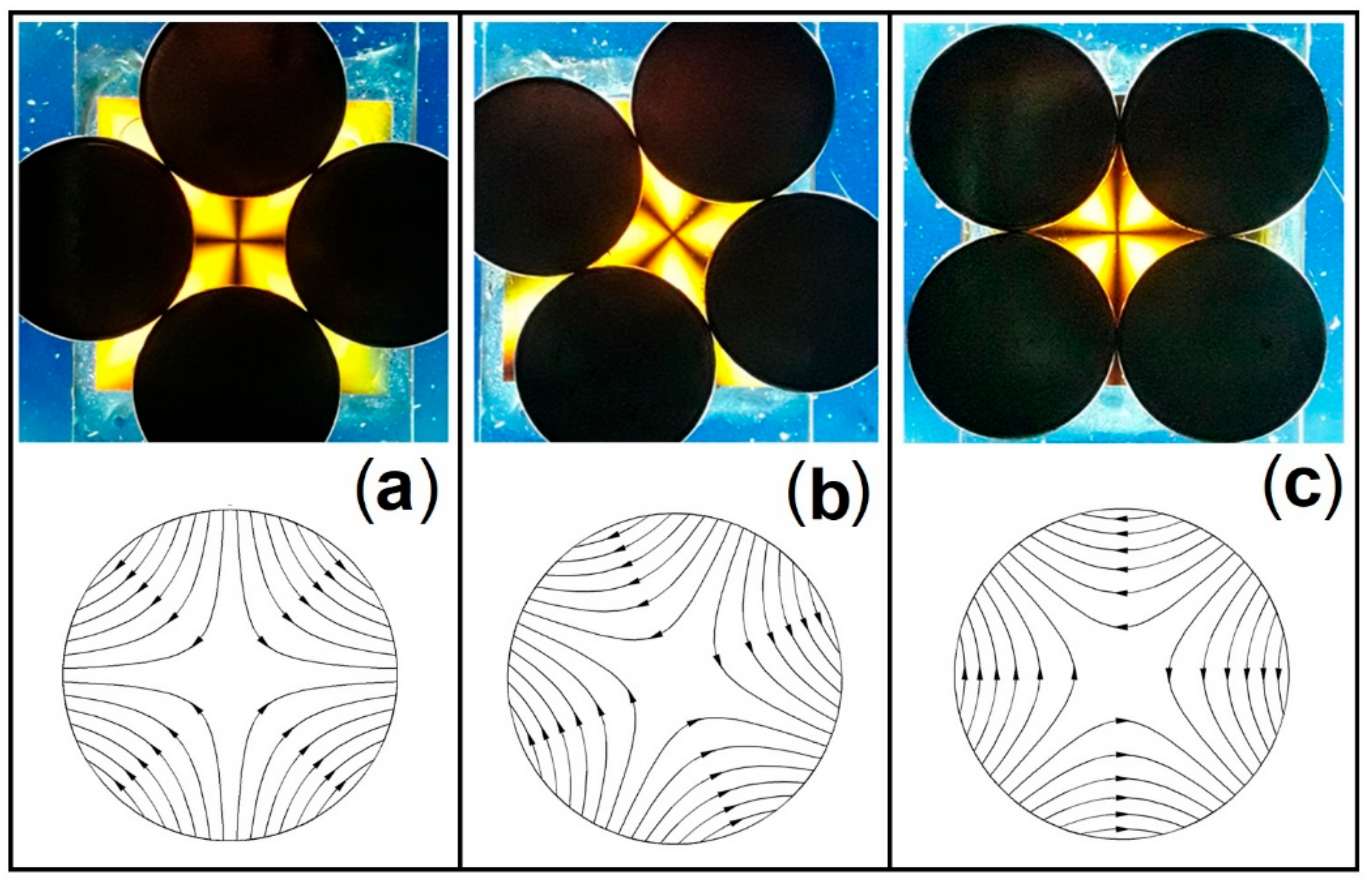
Using other field configurations, we can explore other properties of this magneto-optical system. For example, using a tetrapolar magnetic field setup, we obtained the patterns in Figure 10. We have placed the diagrams of the magnetic field lines together with each light pattern to facilitate the analysis of this system. By rotating this pattern, we observe the curious case of rotation of the isogyres.
We will take Figure 10b above in order to analyze this rotation of the isogyres in comparison with the orientation of the horizontal magnetic field on the Ferrocell plate in Figure 11.
We mark in this luminous pattern the two lines of the isogyres (straight line 1 and straight line 2), as well as the lines of maximum luminous intensity (straight line 3 and straight line 4) in Figure 11a. We can observe these same lines in place of the horizontal magnetic field on the Ferrocell in Figure 11b, along with the tangents of the magnetic field at each crossing point represented by the colors green and yellow for the isogyres, in addition to the colors orange and red for points of maximum luminous intensity.
In the points mentioned above, we can consider that the polarization component of the light that passes through the Ferrocell is parallel to the applied magnetic field. With this information, we observe the same polarization states in the Poincaré sphere shown in Figure 12, and we can obtain the other Stokes parameters associated with each polarization vector obtained by the light scattering of the particles in the ferrofluid.
Furthermore, we obtained the luminous pattern for a hexapolar configuration shown in Figure 13, and we compared it with the polarization states in the magnetic field diagram. Unlike the previous tetrapolar case, where we had two lines of isogyre and two lines of maximum luminous intensity, for the hexapolar case, we have three lines of isogyre intersecting and three lines of maximum intensity.
4. Circular Polarization Characteristics of Light in a Ferrocell
Now we are going to explore some properties of circularly polarized light in a thin film of ferrofluid. According to literature related to light polarization in magnetic fluids, if linearly polarized light passes through ferrofluids under external magnetic fields, the transmitted light can become elliptically polarized depending on the relative orientation between the polarization of the incident light and the applied magnetic field [32].
In order to exemplify the existence of circular polarization of light using Ferrocell, we will explore the phenomena presenting some results. We start our exploration with Figure 14, in which we present a polariscopic system composed of the light passing through a linear polarizer, the Ferrocell, and a circular analyzer, which is a right circular analyzer in the first case and a left circular analyzer in the second one.
The images obtained for the patterns observed are presented in Figure 14d,e for the case of the monopolar configuration. In this figure, we can see in Figure 14c the case for no applied magnetic field, in Figure 14d the pattern obtained for which the analyzer is a left circular device, and for a right circular device in Figure 14c. For Figure 14d,e, the system presents only two dark lobes for each case, in comparison with the previous section with four luminous lobes for the same magnetic field configuration. In addition to that, each pattern is orthogonal to each other. The light intensity is maximum in the diagonal, starting at the top left and ending at the bottom right for the case of the analyzer with left orientation in Figure 14d, and the maximum intensity of light is perpendicular to this diagonal for the case of right circular polarization of Figure 14e.
Continuing our exploration of the existence of elliptical polarization in the Ferrocell, we present another optical arrangement of a circular polariscope using two circular polarizers in opposition in Figure 15a, one left circular polarizer, and the analyzer is a right circular polarizer. In Figure 15b, we have the image of the Ferrocell without an external magnetic field. In Figure 15c, we have the monopolar case for the sequence of optical elements formed by the aright circular polarizer, the Ferrocell, and a left circular analyzer, and for Figure 15d a left circular polarizer, the Ferrocell, and a right circular analyzer. The patterns are similar to the case of Figure 14d,e, but now we can see the existence of different colors, showing that the polarization effect depends on the wavelength of light.
In order to improve our knowledge of the existence of the effects of circular polarized light, we will use the configuration of tetrapolar and hexapolar magnetic fields in Figure 16 and Figure 17.
The most evident result here is that circularly polarized light alternates mainly in regions between the isogyres of linearly polarized light cases if we observe the tetrapolar field diagrams of Figure 16f,g and the hexapolar field of Figure 17g,h. This points to the fact that in the case of partially circularly polarized light, the vertical component of the field going down or up inside the Ferrocell is an important factor and affects the polarization of the light. Comparing the luminous intensities for the cases of linearly polarized light and circularly polarized light, we realize that the light in Ferrocell can present partially polarized light in a circular shape, or more generally, elliptically polarized. To understand this, let us explore some aspects of the Jones vectors for partially polarized light.
Considering a spherical coordinate system associated with a local right-handed Cartesian coordinate system having its origin at the observation point [27], and using Equations (1) and (2), we have the real electric vector with the shape of an ellipse expressed by
where . Thus ∆ is a phase shift parameter. With the ellipsometric interpretation of Stokes parameters expressed as
where and express the orientation of this ellipse. In this way, the electric field of the light is expressed as two-component vector with , here, is an amplitude parameter, not the wavelength [28,29]:
The previous experiment shows that the Ferrocell is an optical element sensitive to polarization described by the operator acting on Jones vectors. The applied magnetic field creating a diffraction grating in the ferrofluid, rotated at angle θM with respect to x-axis is basically a projection on the operator , and the intensity I is the modulus squared of the inner product of this system discussed previously, giving by
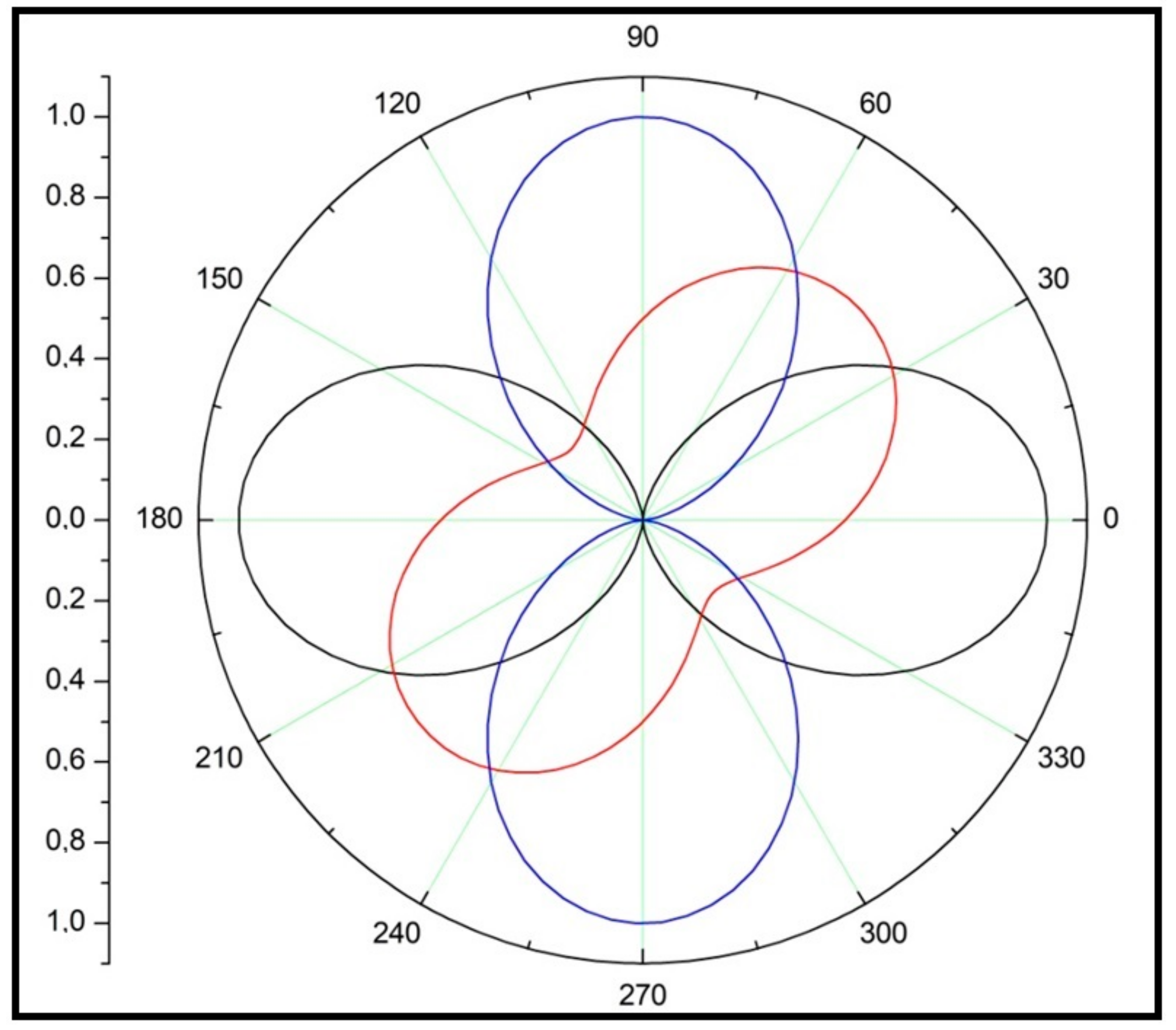
which can represent an ellipse among other geometric shapes. To exemplify this result and make a comparison with the luminous patterns obtained with Ferrocell, we take the following values λ = 0, λ = 1, with ∆ = 0 and λ = with ∆ = π/3, and present them in Figure 18 for the Stokes vector.
Equation (15) says that we have two cases with linearly polarized light effect that occur when we consider λ = 0 (black line) for the angles θM of 0° and 180° and λ = 1 (blue line) in Figure 18. The red line is for λ = , which is the case with circular polarized light effect. With these graphs, we can see that linearly polarized light effect has intensities that pass through the origin (0, 0), meaning the minimal intensity in the light pattern. Whereas the Stokes vector representing circularly polarized light does not pass through the origin. This case of the red line plot represents the observed effects on the light pattern of the right circularly polarized light effect with monopolar applied magnetic field configuration, with maximum intensities at 45° and 225° and minimum intensities at 135° and 315°.
How to explain the simultaneous existence of the linear polarization effect and the circular polarization effect?
The key point here to clarify this apparent contradiction is that we can consider a linearly polarized electromagnetic wave to be the superposition of two opposing circularly polarized waves of equal amplitudes, and we can obtain the equations that describe the independent propagation of both polarized waves circularly to the right and circularly to the left orientation, then we sum the two expressions in a linear superposition with equal amplitude [27,28,29].
Thus, with this polariscope setup, we can see the different components of circular polarization that arise in this system.
For the case of the light patterns obtained with a monopolar configuration of the applied magnetic field to the Ferrocell, we have the configuration for the case of a polarization represented with the red line in Figure 19, in order to exemplify the coexistence of linear and circular polarization of light. Following the method observed in the previous case, we can have light with circularly polarized components for the graphs around the red line (green, red and black curves), which could give us the presence of a linear polarization combined with a circular polarization in the Stokes vector, considering the following function:
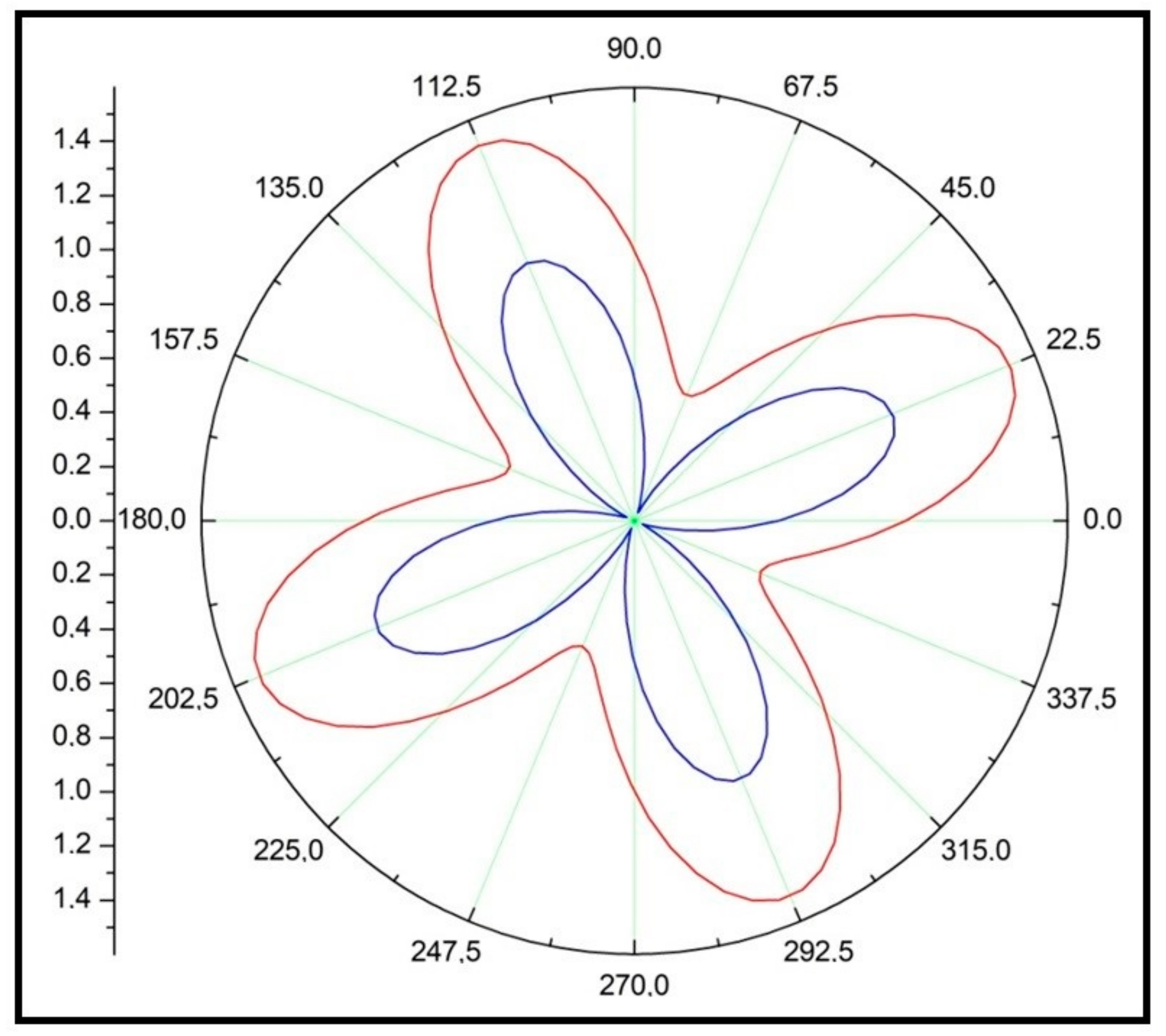
We apply this analysis to the case of light patterns with a hexapolar magnetic field in Figure 20. For the case of right circularly polarized light for the case of the hexapolar magnetic field, we have the Stokes vector intensities graph for a linearly polarized wave in blue, compared to the cases of a wave with partial circular polarization around it represented by the red curve.
In general, these examples show how generalized polarization can be present in the light patterns seen in Figure 14, Figure 15, Figure 16 and Figure 17. A possible explanation for the observation of the presence of these two types of light polarization effects is the dimensionality of the ferrofluid film, one linked to the thickness and the other to the film plane. The linear polarization effect of light is mainly affected by the component of the magnetic field applied to the film plane orienting the ferrofluid microneedles. The birefringence effect occurs due to the phase shift between the two circularly polarized components of light passing through a medium with chiral properties, such as ferrofluids under an applied magnetic field. Thus, the effects of circular polarization are more linked to the component of the magnetic field applied perpendicularly to the film, as shown by the refractive index ellipsoid in Figure 10a of our previous work [3,22,30].
5. Conclusions
Using the polarized light imaging technique, we explored the connections between microscopic film properties and macroscopic properties of light patterns observed from a thin film of ferrofluid subjected to an applied magnetic field. We analyzed patterns of polarized light for different configurations of the applied magnetic field, for example, homogeneous, monopolar, tetrapolar and hexapolar field, and we studied the changing of the polarization of light with the variation of the applied field and their respective Stokes vectors that were represented in Poincaré spheres. We considered that the changes in the dichroism of this system can be monitored throughout the sample, allowing the visualization of magneto-optical effects mainly for linear polarized light. We reported the formation of isogyres and their movement during the rotation of the applied magnetic field. We suggest that the effects of circular polarized light are related to birefringence. Thus, in an almost two-dimensional system of a ferrofluid thin film such as Ferrocell, dichroism would be a more intense effect linked to the effects in the film plane, while the less intense effect of circular polarization would be linked to birefringence due to the thickness of the thin film of ferrofluid. We suggest that this method can be successfully used to investigate the phenomena of particle orientation in ferrofluid thin films, as well as the existence of chiral properties. We have shown how light polarization can be controlled by an applied magnetic field in a Ferrocell.
Author Contributions
All authors contributed to prepare the experiments, propose the mechanisms involved, and analyze the results. The preparation of this manuscript was conducted mainly by A.T. and A.P.B.T. Conceptualization was conducted A.T. and A.P.B.T.; methodology, A.T. and A.P.B.T.; software, A.T., A.P.B.T. and M.S. Editing was conducted by A.T., A.P.B.T. and M.S. All authors have read and agreed to the published version of the manuscript.
Funding
This work was partially supported by Conselho Nacional de Desenvolvimento Científico e Tecnológico (CNPq), Instituto Nacional de Ciência e Tecnologia de Fluidos Complexos (INCT-FCx), and by Fundação de Amparo à Pesquisa do Estado de São Paulo (FAPESP) FAPESP/CNPq#573560/2008-0.
Data Availability Statement
Not applicable.
Acknowledgments
A.T. and A.P.B.T. thank Conselho Nacional de Desenvolvimento Científico e Tecnológico (CNPq), Instituto Nacional de Ciência e Tecnologia de Fluidos Complexos (INCT-FCx), and Fundação de Amparo à Pesquisa do Estado de São Paulo (FAPESP).
Conflicts of Interest
The authors declare no conflict of interest.
References
- Tufaile, A.P.B. Tufaile, A.P.B. Tufaile, Rainbow, Billiards and Chaos. In 11th Chaotic Modeling and Simulation International Conference, 1st ed.; Skiadas, C.H., Lubashevsky, I., Eds.; Springer: Berlin/Heidelberg, Germany, 2019; Volume 1, pp. 289–301. Available online: https://0-link-springer-com.brum.beds.ac.uk/book/10.1007/978-3-030-15297-0 (accessed on 8 March 2022).
- Feynman, R.P.; Leighton, R.B.; Sands, M. The Feynman Lectures on Physics. In The Relativity of Magnetic and Electric Fields; Basic Books: New York, NY, USA, 2011; Volume II, Chapter 13, Section 13–6. [Google Scholar]
- Tufaile, A.; Snyder, M.; Tufaile, A.P.B. Horocycles of Light in a Ferrocell. Condens. Matter. 2021, 6, 30. [Google Scholar] [CrossRef]
- Xia, S.; Wang, J.; Lu, Z.; Zhang, F. Birefringence and magneto-optical properties in oleic acid coated Fe3O4nanoparticles: Application for optical switch. Int. J. Nanosci. 2011, 10, 515–520. [Google Scholar] [CrossRef]
- Candiani, A.; Margulis, W.; Sterner, C.; Konstantaki, M.; Pissadakis, S. Phase-shifted Bragg microstructured optical fiber gratings utilizing infiltrated ferrofluids. Opt. Lett. 2011, 36, 2548–2550. [Google Scholar] [CrossRef] [PubMed]
- Pu, S.; Chen, X.; Chen, L.; Liao, W.; Chen, Y.; Xia, Y. Tunable magnetic fluid grating by applying a magnetic field. Appl. Phys. Lett. 2005, 87, 021901. [Google Scholar] [CrossRef] [Green Version]
- Patel, R.; Mehta, R.V. Ferrodispersion: A promising candidate for an optical capacitor. Appl. Opt. 2011, 50, G17–G22. [Google Scholar] [CrossRef]
- Horng, H.E.; Chieh, J.J.; Chao, Y.H.; Yang, S.-Y.; Hong, C.-Y.; Yang, H.C. Designing optical-fiber modulators by using magnetic fluids. Opt. Lett. 2005, 30, 543–545. [Google Scholar] [CrossRef]
- Zu, P.; Chan, C.-C.; Siang, L.W.; Jin, Y.; Zhang, Y.; Fen, L.H.; Chen, L.; Dong, X. Magneto-optic fiber Sagnac modulator based on magnetic fluids. Opt. Lett. 2011, 36, 1425–1427. [Google Scholar] [CrossRef]
- Pu, S.; Dong, S.; Huang, J. Tunable slow light based on magnetic-fluid-infiltrated photonic crystal waveguides. J. Opt. 2014, 16, 045102. [Google Scholar] [CrossRef]
- Miao, Y.; Wu, J.; Lin, W.; Zhang, K.; Yuan, Y.; Song, B.; Zhang, H.; Liu, B.; Yao, J. Magnetic field tunability of optical microfiber taper integrated with ferrofluid. Opt. Express 2013, 21, 29914–29920. [Google Scholar] [CrossRef]
- Pu, S.; Dong, S. Magnetic Field Sensing Based on Magnetic-Fluid-Clad Fiber-Optic Structure with Up-Tapered Joints. IEEE Photonics J. 2014, 6, 1–6. [Google Scholar] [CrossRef]
- Wang, H.; Pu, S.; Wang, N.; Dong, S.; Huang, J. Magnetic field sensing based on singlemode–multimode–singlemode fiber structures using magnetic fluids as cladding. Opt. Lett. 2013, 38, 3765–3768. [Google Scholar] [CrossRef] [PubMed]
- Chen, Y.; Han, Q.; Liu, T.; Lan, X.; Xiao, H. Optical fiber magnetic field sensor based on sin-gle-mode-multimode-single-mode structure and magnetic fluid. Opt. Lett. 2013, 38, 3999–4001. [Google Scholar] [CrossRef] [PubMed]
- Lin, W.; Miao, Y.; Zhang, H.; Liu, B.; Liu, Y.; Song, B. Fiber-optic in-line magnetic field sensor based on the magnetic fluid and multimode interference effects. Appl. Phys. Lett. 2013, 103, 151101. [Google Scholar] [CrossRef]
- Zu, P.; Chan, C.C.; Lew, W.S.; Hu, L.; Jin, Y.; Liew, H.F.; Chen, L.H.; Wong, W.C.; Dong, X. Temperature-Insensitive Magnetic Field Sensor Based on Nanoparticle Magnetic Fluid and Photonic Crystal Fiber. IEEE Photonics J. 2012, 4, 491–498. [Google Scholar] [CrossRef]
- Deng, M.; Sun, X.; Han, M.; Li, D. Compact magnetic-field sensor based on optical microfiber Michelson interferometer and Fe3O4 nanofluid. Appl. Opt. 2013, 52, 734–741. [Google Scholar] [CrossRef]
- Mehta, R. Polarization dependent extinction coefficients of superparamagnetic colloids in transverse and longitudinal configurations of magnetic field. Opt. Mater. 2013, 35, 1436–1442. [Google Scholar] [CrossRef]
- Philip, J.; Laskar, J.M.; Raj, B. Magnetic field induced extinction of light in a suspension of Fe3O4 nanoparticles. Appl. Phys. Lett. 2008, 92, 229119. [Google Scholar] [CrossRef]
- Tufaile, A.; Vanderelli, T.A.; Tufaile, A.P.B. Light polarization using ferrofluids and magnetic fields. J. Adv. Condens. Matter Phys. 2017, 2017, 2583717. [Google Scholar] [CrossRef] [Green Version]
- Tufaile, A.P.B.; Tufaile, A. Hysteresis Loops, Dynamical Systems and Magneto-Optics. In Chaotic Modeling and Simulation International Conference; Springer: Cham, Switzerland, 2021; pp. 981–993. [Google Scholar] [CrossRef]
- Tufaile, A.; Snyder, M.; Vanderelli, T.A.; Tufaile, A.P.B. Jumping Sundogs, Cat’s Eye and Ferrofluids. Condens. Matter 2020, 5, 45. [Google Scholar] [CrossRef]
- Michael Snyder, Pic2Mag. Available online: https://www.pic2mag.com/ (accessed on 8 March 2022).
- Mendoza-Galván, A.; Muñoz-Pineda, E.; Ribeiro, S.; Santos, M.V.; Järrendahl, K.; Arwin, H. Mueller matrix spectroscopic ellipsometry study of chiral nanocrystalline cellulose films. J. Opt. 2017, 20, 024001. [Google Scholar] [CrossRef] [Green Version]
- Frezza, F.; Mangini, F.; Tedeschi, N. Introduction to electromagnetic scattering: Tutorial. J. Opt. Soc. Am. A 2017, 35, 163–173. [Google Scholar] [CrossRef] [PubMed]
- Riskilä, E.; Lindqvist, H.; Muinonen, K. Light scattering by fractal roughness elements on ice crystal surfaces. J. Quant. Spectrosc. Radiat. Transf. 2021, 267, 107561. [Google Scholar] [CrossRef]
- Mischchenko, M.I.; Travis, L.D.; Lacis, A.A. Scattering, Absorption, and Emission of Light by Small Particles; Cambridge University Press: Cambridge, UK, 2002. [Google Scholar]
- Fowles, G.R. Introduction to Modern Optics, 2nd ed.; Dover: New York, NY, USA, 1975; Available online: https://www.amazon.com.br/Introduction-Modern-Optics-Grant-Fowles/dp/0486659577 (accessed on 8 March 2022).
- Hecht, E. Optics; Addison-Wesley Longman: Boston, MA, USA, 1998; Available online: https://www.amazon.com.br/Optics-Eugene-Hecht/dp/0201116111 (accessed on 8 March 2022).
- Tufaile, A.; Snyder, M.S.; Vanderelli, T.A.; Tufaile, A.P.B. Controlling Light Diffraction with Magnetic Nanostructures, TechConnect Briefs. 2019. Available online: https://briefs.techconnect.org/wp-content/volumes/TCB2019/pdf/116.pdf (accessed on 8 March 2022).
- Gianni Di Domenico and Antoine Weis, Light Polarization and Stokes Parameters. (March 2011). Available online: https://demonstrations.wolfram.com/LightPolarizationAndStokesParameters/ (accessed on 8 March 2022).
- Pu, S.; Dai, M.; Sun, G.; Liu, M. Linear Birefringence and Linear Dichroism Coupled Optical Anisotropy of Magnetic Fluids by External Magnetic Fields. In Proceedings of the 2009 Symposium on Photonics and Optoelectronics, Wuhan, China, 14–16 August 2009; pp. 1–6. [Google Scholar] [CrossRef]
Figure 1.
(a) An example of light pattern in a Ferrocell. This apparatus has a thin film of ferrofluid surrounded by several color LEDs in a circular array around the film. In this case, the magnetic field is applied by an array with 29 cubic magnets. (b) Simulation using Pic2Mag [23] of the magnetic isopotentials produced the magnets.

Figure 2.
The source of the magnetic field in some of our observations of magneto-optical patterns is the use of stacked magnet disks. To increase the field, we make a column of up to six magnets, which increases the magnetic field strength. Placing the disk stack in the center of the Ferrocell with one of its bases facing the glass plate, we have the monopolar magnetic configuration. We present the intensity of the magnetic field in the vertical direction in (a) and in the horizontal direction in (b), in a line situated in the position of the plane where the thin film of ferrofluid is located. The lines show the effect of increasing the field by stacking disks that are shown in the photo of each graph. The magnetic field diagram in (a) shows us that the vertical field is maximum in the central part and decays symmetrically to the left and right. The diagram on the right shows that the magnetic field at the center of the disk is zero and varies symmetrically, but with the sign inverted as an odd function as we move away from the center of the stack of magnetic disks.

Figure 3.
Details of the experimental apparatus. (a) The diagram of one of the polariscope configurations used in this work, in which the light passes through a polarizer, then passes through a ferrofluid film and through a linear analyzer. Throughout the article, we indicate the changes we made in the experimental arrangement. (b) An image of the set with the light diffuser, the polarizer, the Ferrocell, the analyzer, and the magnet. (c) An image of the apparatus, with an open side window showing the polarizers in (a). At the top of the instrument, we have the display in the form of a circular window.

Figure 4.
Diagram of the polariscope with a linear polarizer, Ferrocell, and linear analyzer and respective transfer function.
Figure 4.
Diagram of the polariscope with a linear polarizer, Ferrocell, and linear analyzer and respective transfer function.

Figure 5.
Example of Ferrocell, working as a controllable linear polarizer. In (a), we have the diagram of the parallel lines of the magnetic field between two magnets. In (c), this field is aligned with the polarizer and prevents the passage of light. In (b), we have the same diagram, but with the field lines between the two magnets at 45° of inclination with respect to the polarizer. In (d), we see the light passing with maximum intensity between the two magnets.

Figure 6.
Checking the amplitude of light intensity as a function of angle. Placing a magnetic field in the monopolar configuration in (a), we choose a ring around the center of the magnetic “charge” (BV~1500 G) in (b). A diagram of the field lines is shown in (c). In (d), we have the representation of the luminous intensity as a function of the angle in polar coordinates of the sine squared function.

Figure 7.
Comparison of the model obtained with Malus’ law for a radial diffraction grating with the measurements of light intensity as a function of the angle θ (measured in degrees) obtained experimentally with the Ferrocell.
Figure 7.
Comparison of the model obtained with Malus’ law for a radial diffraction grating with the measurements of light intensity as a function of the angle θ (measured in degrees) obtained experimentally with the Ferrocell.

Figure 8.
In (a), we have the sequence of six images showing the increase in light patterns as a function of the increase in strength of the applied magnetic field. (b) To analyze the effect of increasing the “luminous lobe” we chose a region marked with the red rectangle. (c) Graph of luminous intensity obtained experimentally. The red line represents a fit of an exponentially decaying function to the experimental data. The inset shows a comparison between the image obtained experimentally and a simulation. The first image in (a) and the data of Figure 7 has the same conditions as the experiment shown in the inset in (c). Color shift is an artifact of the camera.

Figure 9.
(a) Graphs of luminous decay as a function of distance for six different values of the applied magnetic field. (b) Graphs of the horizontal magnetic field in the Ferrocell plane region used for the luminous decays are shown above.
Figure 9.
(a) Graphs of luminous decay as a function of distance for six different values of the applied magnetic field. (b) Graphs of the horizontal magnetic field in the Ferrocell plane region used for the luminous decays are shown above.

Figure 10.
At the top, we have light patterns obtained with a tetrapolar magnetic field. At the bottom, we have representations of the corresponding magnetic field lines. In this sequence, we show that the rotation of the tetrapolar magnetic field leads to the rotation of the isogyres pattern. In (a), the central cross of the field is aligned with both the horizontal and the vertical isogyres, in (b), the tetrapolar field has been rotated 22.5° with respect to the previous case, and in (c), the field has been rotated 45° with respect to relative to the first light pattern in (a). In (c), the central cross of the field is not aligned with the isogyres.

Figure 11.
Observing Ferrocell linear polarization in a tetrapolar magnetic field. At each point in the Ferrocell plane, the electromagnetic wave has a characteristic polarization. The points with a minimum light intensity of the isogyres in (a) are represented in the magnetic field diagram (b) by the green and yellow straight segments tangent to these points, marked with the lines (1) and (2). At these points, the magnetic field and microneedles are perpendicular to the polarizer or analyzer. The points with maximum light intensity in (a) are represented with red and orange straight segments in (b), which show that the magnetic field and microneedles are at 45° with respect to the polarizer, marked with lines (3) and (4) in the magnetic field diagram. The magnetic field direction determines the orientation of the polarization of light.

Figure 12.
The Stokes parameters and correspondent Poincaré spheres [31]. The Poincaré sphere is a good representation of the Stokes parameters of Equation (3). The Stokes parameters of a plane electromagnetic wave are always defined with respect to a reference plane containing the direction of wave propagation. The magnetic field induces a rotation in the reference plane around the propagation direction, thus the Stokes parameters are modified according to the rotation transformation rule. The colors red, orange, green, and yellow have the same correspondence as in Figure 11.

Figure 13.
Ferrocell and the hexapolar magnetic field. In (a), we have the light pattern obtained with the Ferrocell in the presence of a symmetrical hexapolar magnetic field in (b), where we can see the formation of three lines of isogyres intersecting. In the magnetic field diagram in (b), we represent the polarization of local light with the green and blue line segments of some of the isogyre lines.

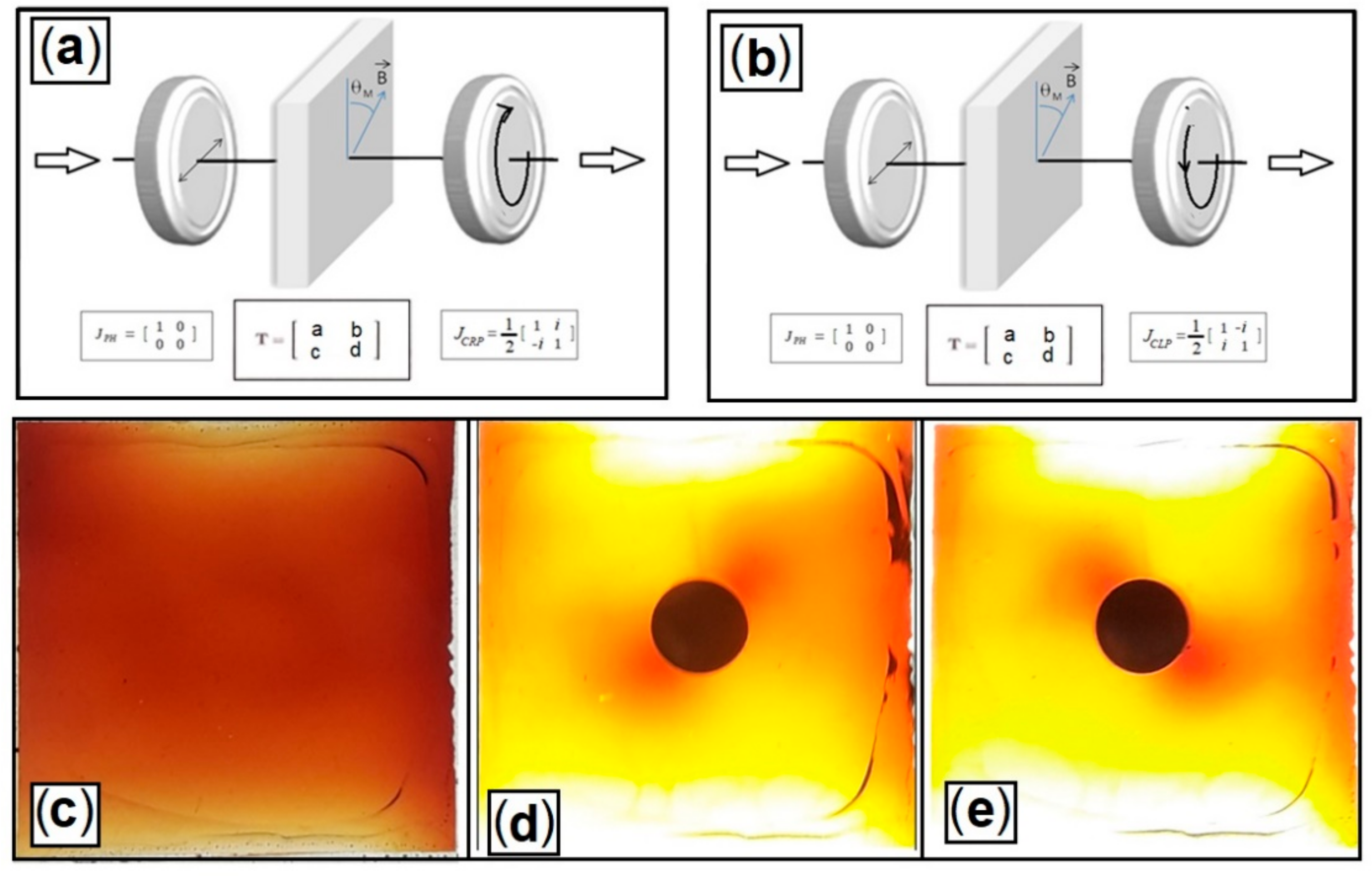
Figure 14.
Circular polarization and the Ferrocell. We used a linear polarizer and a circular analyzer. The polariscopes are used to observe right-handed/clockwise circularly polarized in (a) and left-handed/counterclockwise circularly polarized light in (b). We see in (c) the Ferrocell without a magnetic field, in (d) the light patterns for the right circular polarization cases, and in (e) left circular polarization, using the monopolar magnetic field configuration. Compared with the case of linear polarization, we see that we now have two regions forming darkened lobes instead of having four luminous lobes. Another feature in these patterns is that the lobes seen with the right circular polarization are centered on a diagonal line that is perpendicular to the diagonal where the dark lobes of the left circular polarization are centered.

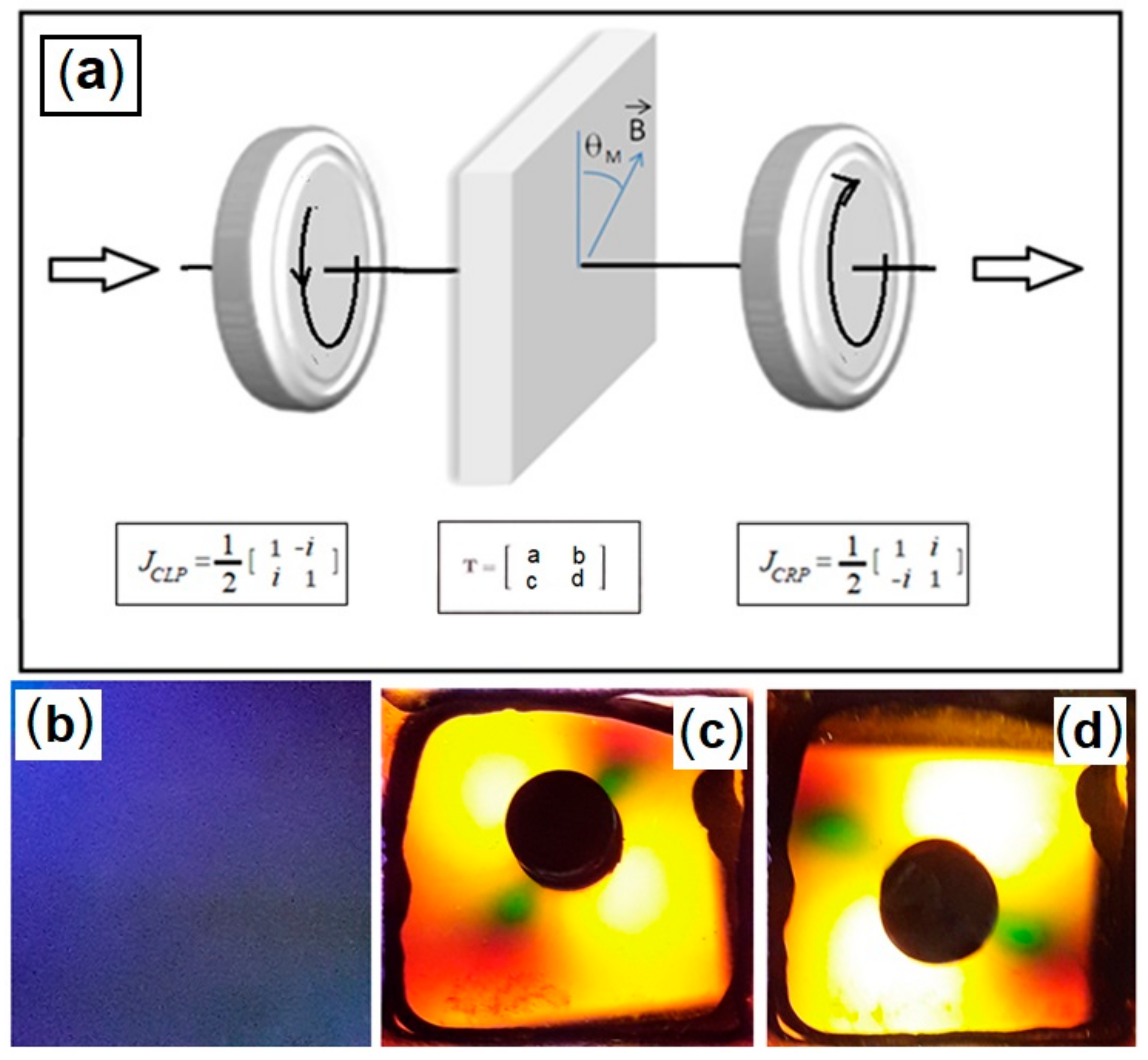
Figure 15.
In this polariscope configuration in (a), we have the diagram of a circular polarizer oriented inversely to the circular analyzer. In (b), we see the polariscope system with the Ferrocell without a magnetic field, with light being practically prevented from passing through the system. In (c), we have a right circular polarizer, a Ferrocell with a monopolar magnetic field, and a left circular analyzer. In (d), we have a left circular polarizer, a Ferrocell with a monopolar magnetic field, and a right circular analyzer. Compared to the previous case, in the current case, we have color separation.

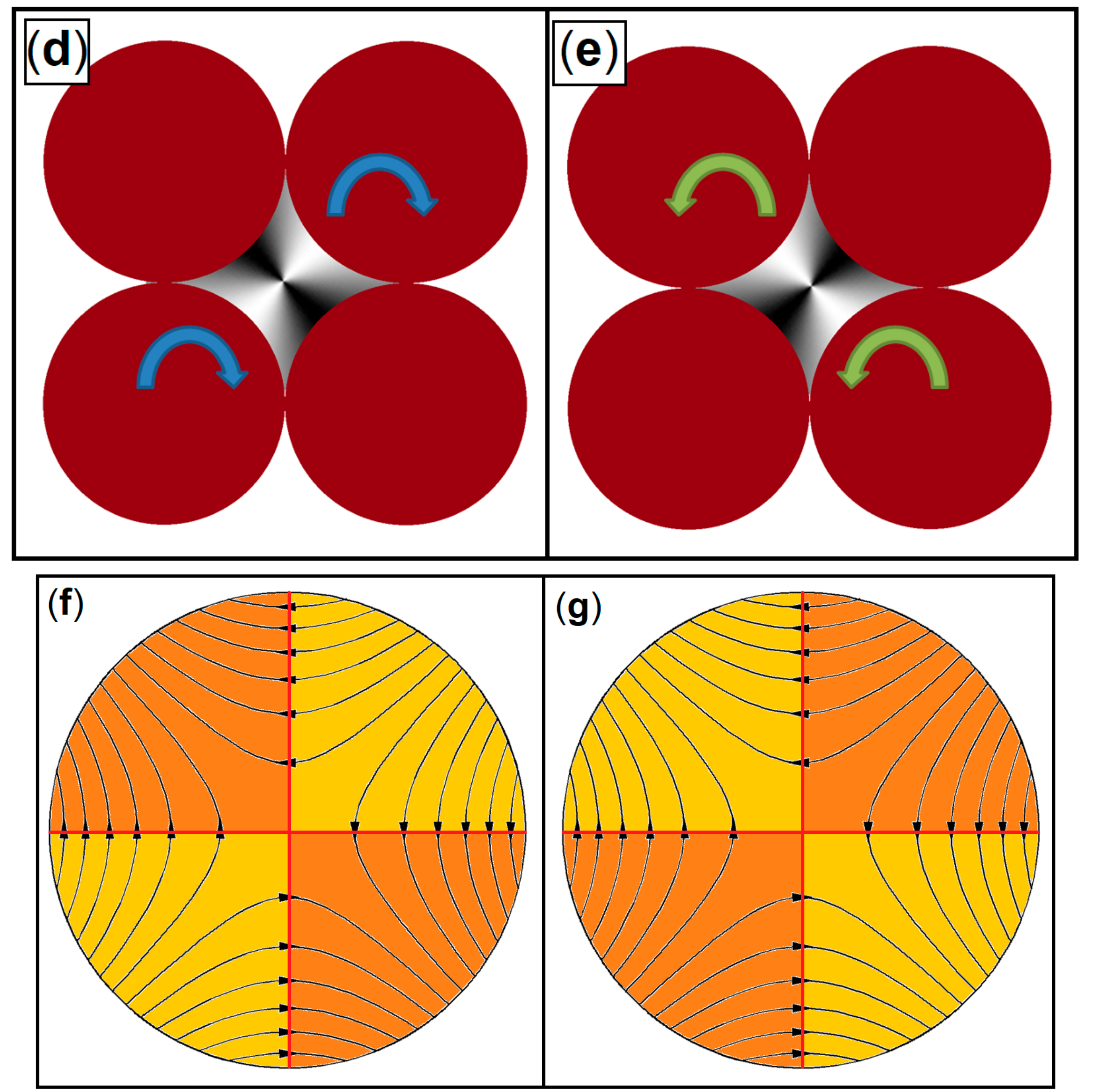
Figure 16.
Circularly polarized light and tetrapolar field in Ferrocell. In these polariscopes, the light passes through a linear polarizer, through Ferrocell with a tetrapolar magnetic field and the analyzer will be changed in each case. In (a), we have a linear analyzer, in (b) a left circular analyzer, and in (c) a right circular analyzer. The diagram in (d) shows left circularly polarized light on one diagonal and the diagram in (e) shows right circularly polarized light on the other diagonal. In (f), (g), we show the magnetic field diagrams for each case of circular polarization orientation, indicating the regions of light intensity decrease with orange color and the intensity increase with yellow color.


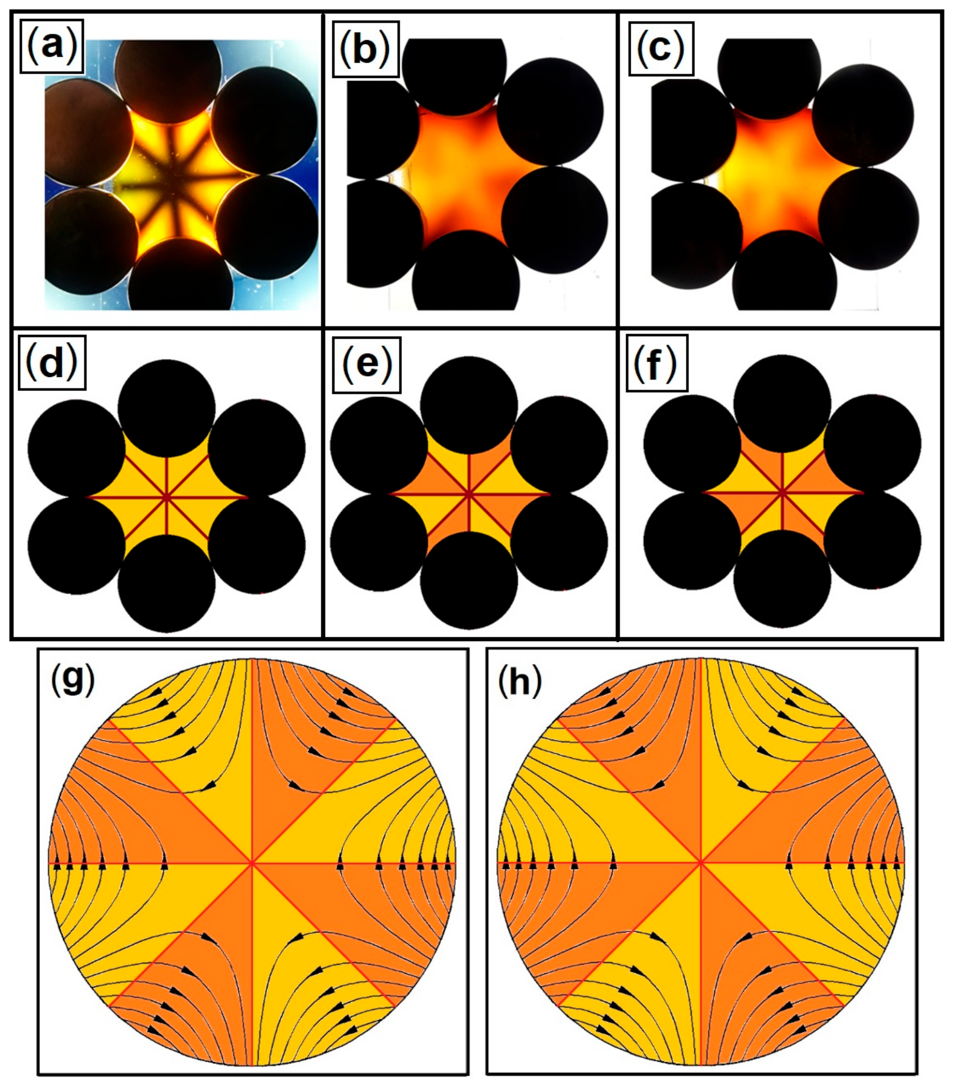
Figure 17.
Circularly polarized light and hexapolar magnetic field in Ferrocell. In (a), we have the case of linear polarization, in (b) the circular polarization to the right, and in (c) the circular polarization to the left. Using yellow color for maximum intensity and orange color for minimum intensity, we show in (d) the diagram for linear polarization, in (e) the right circular polarization, and in (f) the left circular polarization. In (g), we have the diagram of the horizontal magnetic field with the superposition of lighter and darker regions for the right circular polarization and in (h) for the left circular polarization.

Figure 18.
Luminous intensities in polar coordinates for the Stokes vector for the case of ∆ = 0 and λ = 0 (black line) and ∆ = 0 and λ = 1 (blue line) and ∆ = π/3 and λ = 1/ (red line).
Figure 18.
Luminous intensities in polar coordinates for the Stokes vector for the case of ∆ = 0 and λ = 0 (black line) and ∆ = 0 and λ = 1 (blue line) and ∆ = π/3 and λ = 1/ (red line).

Figure 19.
Polar plots for Stokes vector luminous intensity for the function of Equation (17) for ∆ = 0 (red line), ∆ = 0.20 (blue line), ∆ = 0.40 (green line) and ∆ = 0.60 (gray line).
Figure 19.
Polar plots for Stokes vector luminous intensity for the function of Equation (17) for ∆ = 0 (red line), ∆ = 0.20 (blue line), ∆ = 0.40 (green line) and ∆ = 0.60 (gray line).

Figure 20.
The two polar plots of the Stokes vector intensity refer respectively to the polarization states of light for Equation (18) for ∆ = 0.53 (blue line) and for ∆ = 1.00 for (red line).
Figure 20.
The two polar plots of the Stokes vector intensity refer respectively to the polarization states of light for Equation (18) for ∆ = 0.53 (blue line) and for ∆ = 1.00 for (red line).

Publisher’s Note: MDPI stays neutral with regard to jurisdictional claims in published maps and institutional affiliations. |
© 2022 by the authors. Licensee MDPI, Basel, Switzerland. This article is an open access article distributed under the terms and conditions of the Creative Commons Attribution (CC BY) license (https://creativecommons.org/licenses/by/4.0/).
Share and Cite
MDPI and ACS Style
Tufaile, A.; Snyder, M.; Tufaile, A.P.B. Study of Light Polarization by Ferrofluid Film Using Jones Calculus. Condens. Matter 2022, 7, 28. https://0-doi-org.brum.beds.ac.uk/10.3390/condmat7010028
AMA Style
Tufaile A, Snyder M, Tufaile APB. Study of Light Polarization by Ferrofluid Film Using Jones Calculus. Condensed Matter. 2022; 7(1):28. https://0-doi-org.brum.beds.ac.uk/10.3390/condmat7010028
Chicago/Turabian StyleTufaile, Alberto, Michael Snyder, and Adriana Pedrosa Biscaia Tufaile. 2022. "Study of Light Polarization by Ferrofluid Film Using Jones Calculus" Condensed Matter 7, no. 1: 28. https://0-doi-org.brum.beds.ac.uk/10.3390/condmat7010028