
Improvements on Making BKW Practical for Solving LWE †
by
 , , and
Alessandro Budroni
1,* ,
,
Qian Guo
1,2,
Thomas Johansson
2,
Erik Mårtensson
1,2,* and
Paul Stankovski Wagner
2 1
Selmer Center, Department of Informatics, University of Bergen, 5007 Bergen, Norway
2
Department of Electrical and Information Technology, Lund University, 221 00 Lund, Sweden
*
Authors to whom correspondence should be addressed.
†
This paper is an extended version of our paper published in 21st International Conference on Cryptology in India (INDOCRYPT 2020), Bengaluru, India, 13–16 December 2020.
Cryptography 2021, 5(4), 31; https://0-doi-org.brum.beds.ac.uk/10.3390/cryptography5040031
Submission received: 30 September 2021
/
Revised: 22 October 2021
/
Accepted: 26 October 2021
/
Published: 28 October 2021
(This article belongs to the Special Issue Public-Key Cryptography in the Post-quantum Era)
Abstract
:The learning with errors (LWE) problem is one of the main mathematical foundations of post-quantum cryptography. One of the main groups of algorithms for solving LWE is the Blum–Kalai–Wasserman (BKW) algorithm. This paper presents new improvements of BKW-style algorithms for solving LWE instances. We target minimum concrete complexity, and we introduce a new reduction step where we partially reduce the last position in an iteration and finish the reduction in the next iteration, allowing non-integer step sizes. We also introduce a new procedure in the secret recovery by mapping the problem to binary problems and applying the fast Walsh Hadamard transform. The complexity of the resulting algorithm compares favorably with all other previous approaches, including lattice sieving. We additionally show the steps of implementing the approach for large LWE problem instances. We provide two implementations of the algorithm, one RAM-based approach that is optimized for speed, and one file-based approach which overcomes RAM limitations by using file-based storage.
1. Introduction
Since a large-scale quantum computer easily breaks both the problem of integer factoring and the discrete logarithm problem [1], public-key cryptography needs to be based on other underlying mathematical problems. In post-quantum cryptography—the research area studying such replacements—lattice-based problems are the most promising candidates. In the NIST post-quantum standardization competition, 5 out of 7 finalists and 2 out of 8 alternates are lattice-based [2].
The learning with errors problem (LWE) introduced by Regev in [3], is the main problem in lattice-based cryptography. It has a theoretically very interesting average-case to worst-case reduction to standard lattice-based problems. It has many cryptographic applications, including, but not limited to, the design of fully homomorphic encryption schemes (FHE). An interesting special case of LWE is the learning parity with noise problem (LPN), introduced in [4], which has interesting applications in light-weight cryptography.
Considerable cryptanalytic effort has been made when it comes to algorithms for solving LWE. These can be divided into three categories: lattice-reduction, algebraic methods, and combinatorial methods. The algebraic methods were introduced by Arora and Ge in [5], and further considered in [6]. For very small noise, these methods perform very well, but otherwise the approach is inefficient. The methods based on lattice-reduction are The combinatorial algorithms are all based on the Blum–Kalai–Wasserman (BKW) algorithm, and these will be the focus of this paper.
For surveys on the concrete and asymptotic complexity of solving LWE, see [7,8,9], respectively. In essence, BKW-style algorithms have a better asymptotic performance than lattice-based approaches for parameter choices with large noise. Unlike lattice-based approaches, BKW-style algorithms pay a penalty when the number of samples is limited (like in the Darmstadt challenges and many cryptographic schemes). A recent example of a scheme allowing for a very large number of LWE samples can be found in [10].
1.1. Related Work
The BKW algorithm was originally developed as the first subexponential algorithm for solving the LPN problem [11]. In [12], the algorithm was improved, introducing new concepts like LF2 and the use of the fast Walsh–Hadamard transform (FWHT) for the distinguishing phase. A new distinguisher using subspace hypothesis testing was introduced in [13,14].
The BKW algorithm was first applied to the LWE problem in [15]. This idea was improved in [16], where the idea of lazy modulus switching (LMS) was introduced. The idea was improved in [17,18], where [17] introduced so called coded-BKW steps. The idea of combining coded-BKW or LMS with techniques from lattice sieving [19] leads to the next improvement [20]. This combined approach was slightly improved in [9,21]. The distinguishing part of the BKW algorithm for solving LWE was improved by using the fast Fourier transform (FFT) in [22]. One drawback of BKW is its high memory-usage. To remedy this, time-memory trade-offs for the BKW algorithm were recently studied in [23,24,25]. A recent fast implementation of the BKW algorithm for solving LPN is in [26].
1.2. Contributions
In this paper, we introduce a new BKW-style algorithm, including the following.
- A generalized reduction step that we refer to as smooth-LMS, allowing us to use non-integer step sizes. These steps allow us to use the same time, space, and sample complexity in each reduction step of the algorithm, which improves performance compared to previous work.
- A binary-oriented method for the guessing phase, transforming the LWE problem into an LPN problem. While the previous FFT method guesses a few positions of the secret vector and finds the correct one, this approach instead finds the least significant bits of a large amount of positions using the FWHT. This method allows us to correctly distinguish the secret with a larger noise level, generally leading to an improved performance compared to the FFT-based method. In addition, the FWHT is much faster in implementation.
- Concrete complexity calculations for the proposed algorithm showing the lowest known complexity for some parameter choices selected as in the Darmstadt LWE Challenge instances, but with unrestricted number of samples.
- Two implementations of the algorithm that follow two different strategies in memory-management. One is fast, light, and uses solely RAM-memory. The latter follows a file-based strategy to overcome the memory limitations imposed by using only RAM. The file read/write is minimized by implementing the algorithm in a clever way. Simulation results on solving larger instances are presented and verifies the previous theoretical arguments.
1.3. Organization
We organize the rest of the paper as follows. We introduce some necessary background in Section 2. In Section 3, we cover previous work on applying the BKW algorithm to the LWE problem. Then, in Section 4, we introduce our new Smooth-LMS reduction method. Next, in Section 5, we go over our new binary-oriented guessing procedure. Section 6 and Section 7 cover the complexity analysis and implementation of our algorithm, respectively. Section 8 describes our experimental results using the implementation. Finally, the paper is concluded in Section 9.
2. Background
2.1. Notation
Throughout the paper, we use the following notations.
- We write for the base 2 logarithm.
- In the n-dimensional Euclidean space , by the norm of a vector , we consider its -norm, defined asThe Euclidean distance between vectors and in is defined as .
- Elements in are represented by the set of integers in .
- For an linear code, N denotes the code length, and k denotes the dimension.
2.2. The LWE and LPN Problems
The LWE problem [3] is defined as follows.
Definition 1.
Let n be a positive integer, q a prime, and let be an error distribution selected as the discrete Gaussian distribution on with variance . Fix to be a secret vector in , chosen from some distribution (usually the uniform distribution). Denote by the probability distribution on obtained by choosing uniformly at random, choosing an error from and returning
in . The (search)LWEproblem is to find the secret vector given a fixed number of samples from .
The definition above gives the search LWE problem, as the problem description asks for the recovery of the secret vector . Another version is the decision LWE problem, in which case the problem is to distinguish between samples drawn from and a uniform distribution on .
Let us also define the LPN problem, which is a binary special case of LWE.
Definition 2.
Let k be a positive integer, let be a secret binary vector of length k and let be a Bernoulli distributed error with parameter . Let denote the probability distribution on obtained by choosing uniformly at random, choosing from X and returning
The (search)LPNproblem is to find the secret vector given a fixed number of samples from .
Just like for LWE, we can also, analogously, define decision LPN.
Previously, analyses of algorithms solving the LWE problem have used two different approaches. One being calculating the number of operations needed to solve a certain instance for a particular algorithm, and then comparing the different complexity results. The other is asymptotic analysis. Solvers for the LWE problem with suitable parameters are expected to have fully exponential complexity, bounded by as n tends to infinity, where the value of c depends on the algorithms and the parameters of the involved distributions. In this paper, we focus on the complexity computed as the number of arithmetic operations in , for solving particular LWE instances (and we do not consider the asymptotics).
2.3. Discrete Gaussian Distributions
We define the discrete Gaussian distribution over with mean 0 and variance , denoted as the probability distribution obtained by assigning a probability proportional to to each . Then, the discrete Gaussian distribution over with variance (also denoted ) can be defined by folding and accumulating the value of the probability mass function over all integers in each residue class modulo q. It makes sense to consider the noise level as , where . We also define the rounded Gaussian distribution on . This distribution samples values by sampling values from the continuous Gaussian distribution with mean 0 and variance , rounding to the closest integer, and then folding the result to the corresponding value in . We denote it by .
If two independent and are drawn from and respectively, we make the heuristic assumption that their sum is drawn from . We make the corresponding assumption for the rounded Gaussian distribution.
3. A Review of BKW-Style Algorithms
3.1. The LWE Problem Reformulated
Assume that m samples
are collected from the LWE distribution , where . Let and . We have
where , and . The search LWE problem is a decoding problem, where serves as the generator matrix for a linear code over and is a received word. Finding the secret vector is equivalent to finding the codeword for which the Euclidean distance is minimal. In the sequel, we adopt the notation .
3.2. Transforming the Secret Distribution
A transformation [27,28] can be applied to ensure that the secret vector follows the same distribution as the noise. It is done as follows. We write in systematic form via Gaussian elimination. Assume that the first n columns are linearly independent and form the matrix . Define and write Hence, we can derive an equivalent problem described by , where . We compute
Using this transformation, each entry in the secret vector is now distributed according to . The fact that entries in are small is a very useful property in several of the known reduction algorithms for solving LWE.
The noise distribution is usually chosen as the discrete Gaussian distribution or the rounded Gaussian Distribution from Section 2.3.
3.3. Sample Amplification
In some versions of the LWE problem, such as the Darmstadt Challenges [29], the number of available samples is limited. To get more samples, sample amplification can be used. For example, assume that we have M samples , , …, . Then, we can form new samples, using an index set I of size k, as
Given an initial number of samples M, we can produce up to samples. This comes at a cost of increasing the noise level (standard deviation) to . This also increases the sample dependency.
3.4. Iterating and Guessing
BKW-style algorithms work by combining samples in many steps in such a way that we reach a system of equations over of the form , where and the entries are sums of not too many original noise vectors, say , and where t is the number of iterations. The process also reduces the norm of column vectors in to be small. Let denote the number of reduced positions in step i and let . If ; then, every reduced equation is of form
for . The right hand side can be approximated as a sample drawn from a discrete Gaussian, and if the standard deviation is not too large, then the sequence of samples can be distinguished from a uniform distribution. We will then need to determine the number of required samples to distinguish between the uniform distribution on and . Relying on standard theory from statistics, using either previous work [30] or Bleichenbacher’s definition of bias [31], we can find that the required number of samples is roughly
where C is a small positive constant, whose value was studied in [32]. Initially, an optimal but exhaustive distinguisher was used [33]. While minimizing the sample complexity, it was slow and limited the number of positions that could be guessed. This basic approach was improved in [22], using the FFT. This was, in turn, a generalization of the corresponding distinguisher for LPN, which used the FWHT [12]. It was shown in [32] that the FFT distinguisher matches the sample complexity of the optimal distinguisher.
3.5. Plain BKW
The basic BKW algorithm was originally developed for solving LPN in [11]. It was first applied to LWE in [15]. The reduction part of this approach means that we reduce a fixed number b of positions in the column vectors of to zero in each step. In each iteration, the dimension of is decreased by b and after t iterations the dimension has decreased by .
3.6. Coded-BKW and LMS
LMS was introduced in [16] and improved in [18]. Coded-BKW was introduced in [17]. Both methods reduce positions in the columns of to a small magnitude, but not to zero, allowing the reduction of more positions per step. In LMS this is achieved by mapping samples to the same category if the considered positions give the same result when integer divided by a suitable parameter p. In coded-BKW this is instead achieved by mapping samples to the same category if they are close to the same codeword in an linear code, for a suitable value . Samples mapped to the same category give rise to new samples by subtracting them. The main idea [17,18] is that positions in later iterations do not need to be reduced as much as the first ones, giving different values in different steps.
3.7. LF1, LF2, Unnatural Selection
Each step of the reduction part of the BKW algorithm consists of two parts. The first samples are mapped to categories depending on their position values on the currently relevant positions. Next, pairs of samples within the categories are added/subtracted to reduce the current positions to form a new generation of samples. This can be done in a couple of different ways.
Originally, this was done using what is called LF1. Here, we pick a representative from each category and form new samples by adding/subtracting samples to/from this sample. This approach makes the final samples independent, but also gradually decreases the sample size. In [12], the approach called LF2 was introduced. Here, we add/subtract every possible pair within each category to form new samples. This approach requires only 3 samples within each category to form a new generation of the same size. The final samples are no longer independent, but experiments have shown that this effect is negligible.
In [16], unnatural selection was introduced.The idea is to produce more samples than needed from each category, but only keep the best samples, typically the ones with minimum norm on the current positions in the columns of .
3.8. Coded-BKW with Sieving
When using coded-BKW or LMS, the previously reduced positions of the columns of increase in magnitude, with an average factor in each reduction step. This problem was addressed in [20] by using unnatural selection to only produce samples that kept the magnitude of the previous positions small. Instead of testing all possible pairs of samples within the categories, this procedure was sped-up using lattice sieving techniques of [19]. This approach was slightly improved in [9,21].
4. BKW-Style Reduction Using Smooth-LMS
In this section, we introduce a new reduction algorithm solving the problem of having the same complexity and memory usage in each iteration of a BKW-style reduction. The novel idea is to use simple LMS to reduce a certain number of positions and then partially reduce one extra position. This allows for balancing the complexity among the steps, and hence to reduce more positions in total.
4.1. A New BKW-Style Step
Assume having a large set of samples written as before in the form Assume also that the entries of the secret vector are drawn from some restricted distribution with small standard deviation (compared to the alphabet size q). If this is not the case, the transformation from Section 3.2 should be applied. Moreover, in case the later distinguishing process involves some positions to be guessed or transformed, we assume that this has been already considered, and all positions in our coming description should be reduced.
The goal of this BKW-type procedure is to make the norms of the column vectors of small by adding and subtracting equations together in a number of steps. Having expressions of the form , if we can reach a case where is not too large, then can be considered as a random variable drawn from a discrete Gaussian distribution . Furthermore, can be distinguished from a uniform distribution over , if is not too large.
Now, let us describe the new reduction procedure. Fix the number of reduction steps to be t. We will also fix a maximum list size to be , meaning that can have at most columns. In each iteration i, we are going to reduce some positions to be upper limited in magnitude by , for . Namely, these positions that are fully treated in iteration i will only have values in the set of size . We do this by dividing up the q possible values into intervals of length . We also adopt the notation , which describes the number of intervals that we divide the positions up into. We assume that .
4.1.1. First Step
In the first iteration, assume that we have stored . We first compute the required compression starting in iteration 1 by computing (we will explain how later). We then evaluate how many positions that can be fully reduced by computing . The position can be partially reduced to be in an interval of size fulfilling , where . Now, we do an LMS step that “transfers between iterations” in the following way.
We run through all the columns of . For column i, we simply denote it as , and we compute:
The vector is now an index to a sorted list , storing these vectors (The point of inverting all position values if is to make sure that samples that are reduced when added should be given the same index. For example, and are mapped to the same category). Except for the inverting of values if , samples should have the same index if, and only if, all position values are the same when integer divided by ( for the last position). So, we assign . After we have inserted all columns into the list , we go to the combining part.
We build a new matrix in the following way. Run through all indices K and if combine every pair of vectors in by subtracting/adding (Depending on what reduces the sample the most.) them to form a new column in the new matrix . Stop when the number of new columns has reached . For each column in , we have:
- the absolute value of each position is ,
- the absolute value of position is .
4.1.2. Next Steps
We now describe all the next iterations, numbered as . Iteration l will involve positions from to . The very first position has possibly already been partially reduced, and its absolute value is , so the interval for possible values is of the size . Assume that the desired interval size in iteration l is . In order to achieve the corresponding reduction factor , we split this interval in subintervals. We then compute how many positions that can be fully reduced by computing . The position can finally be partially reduced to be in an interval of size fulfilling , where .
Similar to iteration 1, we run through all the columns of . For each column i in the matrix denoted as , we do the following. For each vector position in we compute (here means integer division)
The vector is again an index to a sorted list , keeping track of columns (here, the point of inverting all position values if is to make sure that samples that get reduced when added should be given the same index. For example, and are mapped to the same category). So again, we assign . After we have inserted all column indices into the list , we go to the combining part.
As in the first step, we build a new as follows. Run through all indices K and if combine every pair of vectors by adding/subtracting them to form a column in the new matrix . Stop when the number of new columns has reached .
For the last iteration, since is the last row of , one applies the same step as above, but without reducing the extra position. After t iterations, one gets equations in the form (2), where the vectors in have reduced the norm.
4.2. Smooth-Plain BKW
The procedure described above also applies to plain BKW steps. For example, if in the first iteration, one sets and , then each column vector of will be reduced such that and . Thus, one can either continue with another smooth-plain BKW step by setting also in the second iteration, or switch to smooth-LMS. In both cases, we have the advantage of having already partially reduced. Using these smooth-plain steps, we can reduce a couple of extra positions in the plain pre-processing steps of the BKW algorithm.
4.3. How to Choose the Interval Sizes
To achieve as small a norm of the vectors as possible, we would like the variance of all positions to be equally large, after completing all iterations. Assume that a position x takes values uniformly in the set , for . Thus, we have that . Assuming C is somewhat large, we approximately get . When subtracting/adding two such values, the variance increases to in each iteration. Therefore, a reduced position will have an expected growth of . For this reason, we choose a relation for the interval sizes of the form
This makes the variance of each position roughly the same, after completing all iterations. In particular, our vectors in are expected to have norm at most , and is determined according to the final noise allowed in the guessing phase. Ignoring the pre-processing step with smooth-plain BKW steps; the maximum dimension n that can be reduced is then .
Example 1.
Let and , so . Let us compute how many positions can be reduced using list entries. The idea is that the variance of the right hand side in (2) should be minimized by making the variance of the two terms roughly equal. The error part is the sum of initial errors, so its variance is . In order to be able to distinguish the samples according to (3), we set . This will give us the number of iterations possible as or leading to . Now, we bound the variance of the scalar product part of (2) also to be , so leading to and or if . Then, one chooses , and so on.
4.4. Unnatural Selection
We can improve performance by using the unnatural selection discussed in Section 3.7. Let us make some basic observations. Combining positions using interval size C gives, as previously described, a value in the set , and results in . Combining two vectors from the same category, a position value , where are as above, results in a value in the interval with variance . Now, observe that, for the resulting reduced positions, smaller values are much more probable than larger ones.
4.5. On Optimizing Values
The choice of the parameter within a smooth-LMS step can be optimized in order to achieve a lower number of category in the next step. For example, consider and . The number of categories for a single position would be . Clearly, the same result can be obtained if one chooses . The difference is that with this second choice of , for the same cost (linear on the number of categories), one gets more reduced samples at the end of the step. Therefore, a lower number of categories is required for the next step.
4.6. An Illustration of Smooth Reduction Steps
5. A Binary Partial Guessing Approach
In this section, we propose a new way of reducing the guessing step to a binary version. In this way, we are able to efficiently use the FWHT to guess many entries in a small number of operations. In Section 6 we do the theoretical analysis and show that this indeed leads to a more efficient procedure than all previous ones.
5.1. From LWE to LPN
First, we need to introduce a slight modification to the original system of equations before the reduction part. Assume that we have turned the distribution of to be the noise distribution, through the standard transformation described in Section 3.2. The result after this is written as before
Now, we perform a multiplication by 2 to each equation, resulting in
since, when multiplied with a known value, we can compute the result modulo q.
Next, we apply the reduction steps and make the values in as small as possible by performing BKW-like steps. In our case, we apply the smooth-LMS step from the previous section, but any other reduction method like coded-BKW with sieving would be possible. If the output of this step is a matrix where the Euclidean norm of each is small. The result is written as
where and as before.
Finally, we transform the entire system to the binary case by considering
where is the vector of least significant bits in , the vector of least significant bits in , and denotes the binary error introduced.
We can now examine the error in position j of . In (6), we have equations of the form in , which can be written in integer form as
Now, if , then . In this case, (8) can be reduced mod 2 without error and . In general, the error is computed as . So, one can compute a distribution for by computing . It is possible to compute such distribution, either making a general approximation or precisely for each specific position j using the known values and . Note that the distribution of depends on . Note also that if is reduced to a small norm and the number of steps t is not too large, then it is quite likely that , leading to being large.
For the binary system, we finally need to find the secret value . Either
- there are no errors (or almost no errors), corresponding to . Then, one can solve for directly using Gaussian elimination (or possibly some information set decoding algorithm in the case of a few possible errors).
5.2. Guessing Using the FWHT
The approach of using the FWHT to find the most likely in the binary system in (7) comes directly from previous literature on fast correlation attacks [36].
Let k denote an n-bit vector (also considered as an integer) and consider a sequence , . It can, for example, be a sequence of occurrence values in the time domain, e.g., the number of occurrences of . The Walsh–Hadamard transform is defined as
where denotes the bitwise dot product of the binary representation of the n-bit indices w and k. There exists an efficient method (FWHT) to compute the WHT in time . Given the matrix , we define , where J is the set of all columns of the matrix that equal k. Then, one computes , and we have that corresponds to , such that . In addition, is simply the (biased) sum of the noise terms.
5.2.1. Soft Received Information
The bias of actually depends on the value of . So, a slightly better approach is to use “soft received information” by defining , where is the bias corresponding to . For each , the bias can be efficiently pre-computed so that its evaluation does not affect the overall complexity of the guessing procedure.
5.2.2. Hybrid Guessing
One can use a hybrid approach to balance the overall complexity among reduction and guessing phases. Indeed, it is possible to leave some rows of the matrix unreduced and apply an exhaustive search over the corresponding positions in combination with the previously described guessing step. Since the overall complexity of the algorithm is additive in reduction and guessing phases, one can use hybrid approach to balance the overall complexity among the two. Moreover, we remark that this exhaustive search can easily benefit from parallelization.
5.2.3. Even Selection
When transforming the system to a binary (7), we can zero out some positions to get an easier problem. This can be achieved by ensuring that, when reducing , some specific rows of are small (For a specific entry in a vector and the corresponding value in the secret, we should have ) and additionally have even coefficients, making sure to have enough samples left for the guessing phase. In this way, we cancel out the corresponding entries of when reducing modulo 2 and get a smaller binary system of equations.
5.3. Retrieving the Original Secret
Once is correctly guessed, it is possible to obtain a new LWE problem instance with the secret half as big as follows. Write . Define and . Then, we have that
The entries of have a bit-size half as large as the entries of ; therefore, (10) is an easier problem than (5). One can apply the procedure described above to (10) and guess the new binary secret , i.e., the least significant bits of . The cost of doing this will be significantly smaller, as a shorter secret translates to computationally easier reduction steps. Thus, computationally speaking, the LWE problem can be considered solved once we manage to guess the least significant bits of . Given the list of binary vectors , it is easy to retrieve the original secret .
Generally, if , then , and is nothing else than its binary representation. Conversely, if , then . To compute its magnitude in this case, one must look again at and consider that all negative entries of cannot be reduced any further than . Namely, if for example is negative and at step is reduced to be , then .
The following example shows how to retrieve the original secret once the list of least significant bits vectors has been guessed.
Example 2.
Assume that the secret has length and that its entries’ distribution has standard deviation . Then, performing the above procedure times, with high probability we reduced the secret as much as possible. In the following example, one can note that determines the sign of . Therefore, the magnitude of is retrieved by looking at .
| s0: | ( | 1 | 0 | 0 | 0 | 1 | 1 | 0 | 1 | 0 | 0 | ) |
| s1: | ( | 0 | 0 | 1 | 0 | 0 | 1 | 0 | 1 | 1 | 0 | ) |
| s2: | ( | 1 | 0 | 0 | 0 | 0 | 1 | 1 | 0 | 1 | 1 | ) |
| s3: | ( | 1 | 0 | 0 | 0 | 0 | 1 | 0 | 0 | 1 | 1 | ) |
| s: | ( | −3 | 0 | 2 | 0 | 1 | −1 | 4 | 3 | −2 | −4 | ) |
Note that, if one performs one more iteration, the corresponding binary secret will be the the same as , because we already reached the maximum reduction of possible.
6. Analysis of the Algorithm and Its Complexity
In this section, we describe in detail the newly-proposed algorithm called BKW-FWHT with smooth reduction (BKW-FWHT-SR).
6.1. The Algorithm
The main steps of the new BKW-FWHT-SR algorithm are described in Algorithm 1. We start by changing the distribution of the secret vector with the secret-noise transformation [27], if necessary.
| Algorithm 1 BKW-FWHT with smooth reduction (main framework). |
Input: Matrix with n rows and m columns, received vector of length m and algorithm parameters
|
The general framework is similar to the coded-BKW, with sieving procedure proposed in [20]. In our implementation, we instantiated coded-BKW with sieving steps with smooth-LMS steps discussed before, for the ease of implementation.
The different part of the new algorithm is that after certain reduction steps, we perform a multiplication by 2 to each reduced sample as described in Section 5. We then continue reducing the remain positions and perform the mod 2 operations to transform the entire system to the binary case. Now, we obtain a list of LPN samples and solve the corresponding LPN instance via known techniques, such as FWHT or partial guessing.
One high level description is that we aim to input an LWE instance to the LWE-to-LPN transform developed in Section 5, and solve the instance by using a solver for LPN. To optimize the performance, we first perform some reduction steps to have a new LWE instance with reduced dimension but larger noise. We then feed the obtained instance to the LWE-to-LPN transform.
6.2. The Complexity of Each Step
From now on, we assume that the secret is already distributed as the noise distribution, or that the secret-noise transform is performed. We use the LF2 heuristics and assume the the sample size is unchanged before and after each reduction step. We now start with smooth-plain BKW steps and let be the number of positions already reduced.
6.2.1. Smooth-Plain BKW Steps
Given m initial samples, we could on average have categories (The number of categories is halved compared with the LF2 setting for LPN. The difference is that we could add and subtract samples for LWE) for one plain BKW step in the LF2 setting. Instead, we could assume for categories, and thus, the number of samples m is . Let be the cost of all smooth-plain BKW steps, whose initial value is set to be 0. If a step starts with a position never being reduced before, we can reduce positions, where Otherwise, when the first position is partially reduced in the previous step, and we need categories to further reduce this position, we can in total fully reduce positions, where
For this smooth-plain BKW step, we compute
where is the cost of modulus switching for the last partially reduced position in this step. We then update the number of the reduced positions,
After iterating times, we could compute and . We will continue updating and denote the length reduced by the smooth-plain BKW steps.
6.2.2. Smooth-LMS Steps before the Multiplication of 2
We assume that the final noise contribution from each position reduced by LMS is similar, bounded by a preset value . Since the noise variable generated in the i-th () Smooth-LMS step will be added by times and be multiplied by 2, we compute where is the length of the interval after the LMS reduction in this step. We use categories for one position, where Similar to smooth-plain BKW steps, if this step starts with an new position, we can reduce positions, where Otherwise, when the first position is partially reduced in the previous step and we need categories to further reduce this position, we can in total fully reduce positions, where Let be the cost of Smooth-LMS steps before the multiplication of 2, which is innitialized to 0. For this step, we compute
and then update the number of the reduced positions, .
After iterating times, we compute and . We expect that () positions have been fully reduced and will continue updating .
6.2.3. Smooth-LMS Steps after the Multiplication of 2
The formulas are similar to those for Smooth-LMS steps before the multiplication of 2. The difference is that the noise term is no longer multiplied by 2, so we have for . Moreover, we need to track the a vector of length for the latter distinguisher. The cost is
We also need to count the cost for multiplying samples by 2 and the mod2 operations, and the LMS decoding cost, which are
6.2.4. FWHT Distinguisher and Partial Guessing
After the LWE-to-LPN transformation, we have an LPN problem with dimension and m instance. We perform partial guessing on positions, and use FWHT to recover the remaining positions. The cost is,
6.3. The Data Complexity
We now discuss the data complexity of the new FWHT distinguisher. In the integer form, we have the following equation,
If then . Then, the equation can be reduced mod 2 without error. In general, the error is .
We employ a smart FWHT distinguisher with soft received information, as described in Section 5. From [37], we know the sample complexity can be approximated as
For a different value of , the distribution of is different. The maximum bias is achieved when . In this sense, we could compute the divergence as
where is the Bernoulli variable conditioned on the value of z and the uniform distribution over the binary field.
Following the previous research [15], we approximate the noise as discrete Gaussian with standard deviation . If is large, the probability is very close to . Then, the expectation can be approximated as
i.e., the divergence between a discrete Gaussian with the same standard deviation and a uniform distribution over , . We numerically computed that the approximation is rather accurate when the noise is sufficiently large (see Table 1). In conclusion, we use the formula
to estimate the data complexity of the new distinguisher. It remains to control the overall variance . Since we assume that the noise contribution from each reduced position by LMS is the same and the multiplication of 2 will double the standard deviation, we can derive
Note: The final noise is a combination of three parts, the noise from the LWE problem, the LMS steps before the multiplication by 2, and the LMS steps after the multiplication by 2. The final partial key recovery problem is equivalent to distinguishing a discrete Gaussian from uniform with the alphabet size doubled. We see that with the multiplication by 2, the variances of the first and the second noise parts are increased by a factor of 4, but the last noise part does not expand. This intuitively explains the gain of the new binary distinguisher.
6.4. In Summary
We have the following theorem to estimate the complexity of the attack.
Theorem 1.
The time complexity of the new algorithm is
under the condition that
where .
6.5. Numerical Estimation
We numerically estimate the complexity of the new algorithm BKW-FWHT-SR (shown in Table 2). It improves the known approaches when the noise rate (represented by ) becomes larger. We should note that, compared with the previous BKW-type algorithms, the implementation is much easier, though the complexity gain might be mild.
7. Implementations
We produced two different C implementations of the BKW algorithm, as presented in this manuscript. These mainly differ in memory management. The first one, referred to as RBBL (RAM-based BKW for LWE), is light, fast, and relies only on RAM usage. However, this turned out to be a limiting factor for solving hard LWE instances. Therefore, the second implementation, referred to as FBBL (file-based BKW for LWE), follows a design strategy that can be seen as a transition away from such a limiting factor. The main idea is to use a file-based approach to store the samples, moving the memory constraint from RAM to disk capacity. More details are given in the next sections. Both implementations are available as open-source libraries at https://github.com/FBBL, accessed on 25 October 2021. Some simulation results are presented in Section 8.
7.1. RAM-Based Implementation
Storing samples directly in RAM allows a simple and fast implementation. The purpose of RBBL is to achieve good results in solving relatively small LWE instances and provide a comparison against the file-based solution FBBL. RBBL supports Smooth-LMS reduction steps, including smooth-plain BKW steps. The FWHT-based guessing method introduced in Section 4 and Section 5 is implemented in both its plain and hybrid version.
7.1.1. Memory and Sample Organization
The samples are stored in heap within a single array, allowing for a single (and faster) memory allocation. For each category, we allocate enough memory to fit a fixed number of samples. Therefore, if for a certain category, the number of new samples exceeds the category capacity, some samples are discarded.
7.1.2. Parallelization
RBBL supports parallelization using the POSIX Threads utility. Within the steps of the reduction phase, each thread gets assigned to different sets of categories and performs sums and subtractions of samples independently. A system of mutexes prevents memory corruption caused by two or more threads writing to the same category, and therefore to the same memory cells, at the same time. The guessing phase benefits from parallelization when using the hybrid guesser. All the possible combinations of entries of the bruteforce positions are equally distributed among the available threads, which perform an FWHT for each one of them. Finally, one chooses the guess paired with the highest probability, as explained in Section 5.2.
7.2. File-Based Implementation
A file-based implementation is needed when the amount of memory required to store the samples exceeds the available RAM. FBBL supports most known BKW reduction steps, FFT and FWHT-based guessing methods, and hybrid guessing approaches. Different reduction steps can be combined arbitrarily, and the implementation also allows full recovery of the initial secret, including the initial transform and guessing all parts of the secret vector (if all intermediate reduction results have been stored and are compatible). A key success factor in the software design was to avoid unnecessary reliance on RAM, so we have employed file-based storage where necessary and practically possible. We describe below how we dealt with some interesting performance issues.
7.2.1. File-Based Sample Storage
Samples get stored in a file, sorted according to their category. The necessary space for a fixed number of samples is reserved into the file for each category. Then, a storage writer writes down the samples from RAM to file in the space reserved for their categories (possibly discarding some samples if they are full or leaving some empty space otherwise). A category mapping, unique for each reduction type, defines what category index a given sample belongs to (In this section, a category is defined slightly differently from the rest of the paper. A category together with its adjacent category are together what we simply refer to as a category in the rest of the paper).
When samples are combined in the reduction step, we can either subtract or add them together. The subtraction of samples is performed within a single category, while addition needs to take two samples from adjacent categories. For example, considering how plain-BKW reduction works for just one position with modulus q, there are q different categories, one for each position value. Samples in categories a and are adjacent, since they cancel out (at that position) when added together. The category mapping is constructed so that adjacent categories are stored as neighbors on file, in order to maintain a sequential access pattern, avoiding the need for random accesses on file.
Consider one BKW reduction step. A reduction step takes a sample file as input and produces a new sample file as output. The fast dual SSDs of our target machine are used for efficiency here, reading from the source file, writing to the destination file. Sample reading is performed sequentially from beginning to end of file. This is very straightforward, reading a pair of adjacent categories into memory, processing them (the reduction), and writing the resulting samples to (another) file. Writing samples to the destination file is much more elaborate, utilizing as much of the RAM as is available as a buffer, flushing to disk with one sequential write to the destination file. This needs to be done whenever the buffer fills up, generally, but depending on the problem parameters, the amount of RAM and disk memory used, requiring multiple flushes.
7.2.2. Optional Sample Amplification
We support optional sample amplification. That is, if a problem instance has a limited number of initial samples (e.g., the Darmstadt LWE challenge), then it is possible to combine several of these to produce new samples (more, but with higher noise).
While this is very straightforward in theory, we have noticed considerable performance effects when this recombination is performed naïvely. For example, combining triplets of initial samples using a nested loop is problematic in practice for some instances, since some initial samples become over-represented—some samples are used more often than others when implemented this way.
We have solved this by using a linear feedback shift register to efficiently and pseudo-randomly distribute the selection of initial samples more evenly.
7.2.3. Employing Meta-Categories
For some LWE problem instances, using a very high number of categories with few samples in each is a good option. This can be problematic to handle in an implementation, but we have used meta-categories to handle this situation. For example, using plain BKW reduction steps with modulus q and three positions, we end up with different categories. With q large, an option is to use only two out of the three position values in a vector to first map it into one out of different meta-categories. When processing the (meta-)categories, one then needs an additional pre-processing in the form of a sorting step in order to divide the samples into their respective (non-meta) categories (based on all three position values), before proceeding as per usual.
We have used this implementation trick to, for example, implement plain BKW reduction for three positions. One may think of the process as brute-forcing one out of three positions in the reduction step.
7.2.4. Parallelization
The hybrid FWHT-based guessing method benefits from parallelization similarly to the hybrid guesser in the RBBL implementation. To every available thread we assign an equal number of possible guesses for the bruteforced part. Each thread independently runs an FWHT, and the most likely guess among all threads is chosen as the solution. Due to our focus on storage-related sample processing, we have not yet parallelized the BKW steps. This would require more effort compared to the RBBL case, since one would want to parallelize the writing-to-file part too. It is in our future plan to work on it.
7.3. A Novel Idea for Fast Storage Writing
Here, we introduce a new approach to handle file-based sample storage, which is particularly efficient for SSDs. That is, we describe a procedure for writing samples to physical storage in an efficient way for large LWE instances with many samples. It is intended to be used in future implementations.
7.3.1. Intuition
The main idea is to utilize the fact that disk access has a much lower time penalty for SSD disks than for classical mechanical disks. In other words, we make use of the fact that SSDs act more like random access memory.
On a high level, the idea is to bunch several categories together into a well-chosen number of meta-categories. This can be done in a very general way, simply by grouping the category indices into intervals of suitable length (depending on available memory). We then make a rough sorting into these meta-categories, where we keep the samples unsorted (within their respective meta-category). For every such meta-category, we utilise a separate file handle, so we have, say, w different write positions on disk. The gain here is that we can simply employ the rough sorting and then directly flush each newly created sample (or batches of them if buffering is employed) into their respective file by appending. As mentioned, this technique works better for SSD-type disks than mechanical ones, because there is a penalty for physically moving the write head for every append operation. Of course, this can partially be dealt with by buffering the outputs, but this is a trade-off issue between the performance gain of the algorithm itself versus the performance penalties of moving between the w different write positions, which explains why the solution is more interesting for SSD storage.
7.3.2. Technical Description
Assume we have a table in RAM and a larger table on disk denoted . Then, one splits the list of size into different parts, where M is related to the maximum RAM that can be used. Clearly, one such part matches the maximum RAM size, i.e., one part contains as many entries as can be contained in RAM.
Define a simple map , where . A table in RAM is created and contains m storage units denoted , . When reading column i from , one computes the corresponding index K according to Equation (4) for the column x, and then the file part by . The column vector x is then stored in the storage units .
Once the table is full, we append the parts to the larger table on disk , again containing m storage units denoted , . Store the content of in , appended to previous content, for . Therefore, the table is now empty and ready to start over again and read columns of .
In the combining step, we read the content of one to RAM. However, because the content is not fully sorted, we now address the table by the K values instead. Assume that now is sorted according to K. Step through , and for all entries with the same K value, we create all combinations of differences between these vectors. Write them to a new in successive order.
7.4. Other Implementation Aspects
Some more things to consider implementation-wise are the following.
7.4.1. Strict Unnatural Selection
There are advantages to performing very strict unnatural selection in the last reduction step, drastically reducing the total number of samples. First of all, this allows us to reduce more positions and/or reduce the positions to a much lower magnitude. Secondly, having much fewer samples speeds up the FWHT distinguisher, allowing us to brute-force guess more positions.
We leave investigating the idea of applying aggressive unnatural selection in each step, in other words coded-BKW with sieving, for future implementation work.
7.4.2. Skipping the All 0 s Guess When Using the FWHT Distinguisher
Consider the guess where all the LSBs of the secret are equal to 0. For that guess, (9) simplifies to
Since even values of are more common than odd values, this sum is biased, meaning that the FWHT is much more likely to choose this guess. Since it is exceptionally unlikely that this guess is the correct one, we can improve the distinguisher by simply discarding this guess.
7.4.3. FWHT Distinguisher When the RAM Is a Limitation
Suppose that the FWHT distinguisher is applied on n positions, where the corresponding values are too many to store in RAM. It is possible to do a binary brute-force search over r of the position values of (9) and calculate an FWHT with only bits for each of the possible bit sequences. This approach reduces the space complexity of the algorithm from to
The time complexity of the normal FWHT distinguisher, including the cost of processing the m samples to calculate the values, is
When brute-forcing r positions, we need to iterate over all m samples and calculate a scalar product of r positions, and calculate an FWHT of bits, for each of the guesses. This leads to a time complexity of
7.4.4. On the Minimum Population Size
It turns out that it is possible to use slightly fewer samples than a worst-case analysis would imply. The samples after a reduction step are not completely evenly spread out among the categories. The overproduction of categories with extra samples overcompensates for the lack of production from categories with few samples. The uneven spread of samples is due to two factors.
- By design, a small fraction of the categories will get fewer samples on average.
- Even ignoring the first point, the spread will, due to randomness, not be perfectly even.
Let us analyze the situation in detail. Assume that we have N categories, M samples and that the probability of a sample being mapped to category i is , where . Let denote the number of samples in category i and denote the number of samples produces in category i. With this notation, the expected new samples being produced are:
The number of samples in category i are . Using well-known formulas for the mean and the variance of the binomial distribution, we get
leading to a total expected production of
Setting the production equal to M and solving for M gives us
Notice here that the further away from uniformly random the values are, the smaller we need M to be. Assuming that all categories have , we get
We can thus keep the sample size constant using samples, gaining a factor of over a worst-case analysis, which assumes that we need samples. Notice that we gain from this effect even if we use larger values of M than needed, and choose the best samples using unnatural selection.
8. Experimental Results
In this section, we report some of the experimental results obtained in solving real LWE instances with varying parameters. Our main goal was to confirm our theory and to prove that BKW algorithms can be used in practice to solve relatively large instances. For the case of FBBL, there is still room to run a more optimized code and possibly to make more optimal parameter choices. However, the results show that the BKW algorithm is practical, and that its performances are on a comparable scale to the ones from lattice-based approaches.
We considered two different scenarios. In the first case, we assumed for each LWE instance to have access to an arbitrary large number of samples. Here, we create the desired amount of samples ourselves (we used rounded Gaussian noise for simplicity of implementation). In the second case, we considered instances with a limited number of samples. An LWE problem is considered solved when the binary secret is correctly guessed, for reasons explained in Section 5.3.
8.1. Target Machine
For our file-based experiments, we assembled a machine, that will be referred as machine A, to achieve a high speed in file reading/writing. We used an ASUS PRIME X399-A motherboard, a 4.0 GHz Ryzen Threadripper 1950X processor, and 128 GiB of 2666 MHz DDR4 RAM. For storage, we used a separate (slow) SSD Samsung 860 QVO for the operating system (Windows 10), an Ultrastar HE12 12TB SATA mechanical disk, and dual (fast) SSDs SAMSUNG 970 EVO Plus 2TiB NVMe M.2 internal. While the machine is built from standard parts with a limited budget, we have primarily attempted to maximize the amount of RAM and the size and read/write speeds of the fast SSDs for the overall ability to solve large LWE problem instances.
For the RAM-based experiments, we switched to a machine equipped with a faster processor. We used a desktop with processor 3.60 GHz Intel Core i7-7700 CPU, running Linux Mint 20 and with 32 GB of RAM. We will refer to this second machine as machine B.
8.2. Unlimited Number of Samples
We targeted the parameter choices of the TU Darmstadt challenges [29]. For each instance, we generated as many initial samples as needed according to our estimations. In Example 3, we present our parameter choices for one of these. In Table 3, we report the details of the largest solved instances. One can see that RBBL achieves considerably faster results than FBBL, both when comparing them on the same machine B, and when FBBL runs on machine A. This gives us an idea of how much the results obtained using FBBL on larger LWE instances could be improved if using RBBL on a machine with a larger RAM available.
Example 3.
Let us consider an LWE instance with , and . To successfully guess the secret, we first performed 8 smooth-plain BKW steps, reducing 17 positions to zero. We used the following parameters.
Note that . In this way, we exploited the smoothness to zero for one additional position. For this reason, we start step 6 by skipping one position. Finally, we did 5 smooth-LMS steps using the following parameters:
These parameters are chosen in such a way that the number of categories (The number of categories here is the double of what is explained in previous sections since opposite samples are put in different categories in the implementation) is ≈ in the early stages and ≈ at most. We started with samples that guaranteed us to end up with enough samples for guessing the right solution. The last position is brute-forced and therefore left untouched at the last reduction step.
8.3. Limited Number of Samples
We solved the original TU Darmstadt LWE challenge instance [29] with parameters , and the number of samples limited to . We did this by forming 140 million samples using sample amplifying with triples of samples, taking 6 steps of smooth-plain BKW on 14 entries, followed by 6 steps of smooth-LMS on 25 entries. The final position was left to brute force. The overall running time, obtained with FBBL on machine A, was 55 min.
9. Conclusions and Future Work
We introduced a novel and easy approach to implementing a BKW reduction step, which allows balancing the complexity among the iterations, and an FWHT-based guessing procedure able to correctly guess the secret with relatively large noise level. Together with a file-based approach of storing samples, the above define a new BKW algorithm specifically designed to solve practical LWE instances, where the available RAM is typically a limiting factor.
With an implementation of the file-based algorithm, we managed to solve 6 challenges with Darmstadt challenge-type parameters, but with an unlimited number of samples, 3 more challenges than in the conference version of the paper [38]. For the 3 previously solved challenges, we made substantial improvements in runtime.
We also managed to solve the easiest Darmstadt challenge, in its original form.
Furthermore, we implemented a fully RAM-based version of the new algorithm, to compare against the file-based approach, in settings where the available RAM was not a limiting factor. We leave it to future work to experiment with such implementation, with harder LWE instances on machines with larger RAM available.
We did parallelize the FWHT and the RAM-based version of the algorithm, but we leave more parallelization work and other optimization work for the future.
While we managed to substantially improve the implementation results of the conference version of the paper [38], we believe that significant improvements to the algorithm can still be made to reduce the gap compared to lattice-based techniques for solving LWE. For example, it remains to investigate the concrete improvement of employing the sieving aspect of coded-BKW with sieving [20]. Moreover, the investigation of the specific design of the BKW algorithm for handling the problem of few initial samples is left for future work.
Author Contributions
Conceptualization, T.J.; software, A.B., E.M. and P.S.W.; validation, all authors; formal analysis, Q.G.; investigation, all authors; writing—original draft preparation, all authors; writing—review and editing, all authors; project administration, T.J., Q.G. and P.S.W.; funding acquisition, T.J., Q.G. and P.S.W. All authors have read and agreed to the published version of the manuscript.
Funding
This work was supported in part by the Swedish Research Council (Grant No. 2019-04166), the Norwegian Research Council (Grant No. 247742/070), and the Swedish Foundation for Strategic Research (Grant No. RIT17-0005 and strategic mobility grant No. SM17-0062). This work was also partially supported by the Wallenberg AI, Autonomous Systems and Software Program (WASP) funded by the Knut and Alice Wallenberg Foundation. Finally, this work is partially supported by the project “Kvantesikker Kryptografi” from the National Security Authority of Norway.
Institutional Review Board Statement
Not applicable.
Informed Consent Statement
Not applicable.
Data Availability Statement
The data presented in this study are available in article.
Conflicts of Interest
The authors declare no conflict of interest.
References
- Shor, P.W. Algorithms for Quantum Computation: Discrete Logarithms and Factoring. In Proceedings of the 35th Annual Symposium on Foundations of Computer Science, Santa Fe, NM, USA, 20–22 November 1994; pp. 124–134. [Google Scholar] [CrossRef]
- NIST Post-Quantum Cryptography Standardization. Available online: https://csrc.nist.gov/Projects/Post-Quantum-Cryptography/Post-Quantum-Cryptography-Standardization (accessed on 24 September 2018).
- Regev, O. On lattices, learning with errors, random linear codes, and cryptography. In Proceedings of the 37th Annual ACM Symposium on Theory of Computing, Baltimore, MD, USA, 22–24 May 2005; Gabow, H.N., Fagin, R., Eds.; ACM Press: Baltimore, MA, USA, 2005; pp. 84–93. [Google Scholar] [CrossRef]
- Blum, A.; Furst, M.L.; Kearns, M.J.; Lipton, R.J. Cryptographic Primitives Based on Hard Learning Problems. In Advances in Cryptology—CRYPTO’93; Stinson, D.R., Ed.; Lecture Notes in Computer Science; Springer: Heidelberg, Germany; Santa Barbara, CA, USA, 1994; Volume 773, pp. 278–291. [Google Scholar] [CrossRef] [Green Version]
- Arora, S.; Ge, R. New Algorithms for Learning in Presence of Errors. In Proceedings of the ICALP 2011: 38th International Colloquium on Automata, Languages and Programming, Part I, Zurich, Switzerland, 4–8 July 2011; Aceto, L., Henzinger, M., Sgall, J., Eds.; Lecture Notes in Computer Science; Springer: Heidelberg, Germany; Zurich, Switzerland, 2011; Volume 6755, pp. 403–415. [Google Scholar] [CrossRef]
- Albrecht, M.; Cid, C.; Faugere, J.C.; Fitzpatrick, R.; Perret, L. On the complexity of the Arora-Ge algorithm against LWE. In Proceedings of the SCC 2012–Third international conference on Symbolic Computation and Cryptography, Castro Urdiales, Spain, 11–13 July 2012. [Google Scholar]
- Albrecht, M.R.; Player, R.; Scott, S. On the concrete hardness of Learning with Errors. J. Math. Cryptol. 2015, 9, 169–203. [Google Scholar] [CrossRef] [Green Version]
- Herold, G.; Kirshanova, E.; May, A. On the asymptotic complexity of solving LWE. Des. Codes Cryptogr. 2018, 86, 55–83. [Google Scholar] [CrossRef]
- Guo, Q.; Johansson, T.; Mårtensson, E.; Stankovski Wagner, P. On the Asymptotics of Solving the LWE Problem Using Coded-BKW With Sieving. IEEE Trans. Inf. Theory 2019, 65, 5243–5259. [Google Scholar] [CrossRef]
- Katsumata, S.; Kwiatkowski, K.; Pintore, F.; Prest, T. Scalable Ciphertext Compression Techniques for Post-quantum KEMs and Their Applications. In Advances in Cryptology—ASIACRYPT 2020; Moriai, S., Wang, H., Eds.; Springer International Publishing: Cham, Switzerland, 2020; pp. 289–320. [Google Scholar]
- Blum, A.; Kalai, A.; Wasserman, H. Noise-tolerant learning, the parity problem, and the statistical query model. In Proceedings of the 32nd Annual ACM Symposium on Theory of Computing; Portland, OR, USA, 21–23 May 2000, ACM Press: Portland, OR, USA, 2000; pp. 435–440. [Google Scholar] [CrossRef]
- Levieil, É.; Fouque, P.A. An Improved LPN Algorithm. In Proceedings of the SCN 06: 5th International Conference on Security in Communication Networks, Maiori, Italy, 6–8 September 2006; Prisco, R.D., Yung, M., Eds.; Lecture Notes in Computer Science. Springer: Heidelberg, Germany; Maiori, Italy, 2006; Volume 4116, pp. 348–359. [Google Scholar] [CrossRef]
- Guo, Q.; Johansson, T.; Löndahl, C. Solving LPN Using Covering Codes. In Advances in Cryptology—ASIACRYPT 2014, Part I; Sarkar, P., Iwata, T., Eds.; Lecture Notes in Computer Science; Springer: Heidelberg, Germany; Kaoshiung, Taiwan, 2014; Volume 8873, pp. 1–20. [Google Scholar] [CrossRef]
- Guo, Q.; Johansson, T.; Löndahl, C. Solving LPN Using Covering Codes. J. Cryptol. 2020, 33, 1–33. [Google Scholar] [CrossRef] [Green Version]
- Albrecht, M.R.; Cid, C.; Faugère, J.; Fitzpatrick, R.; Perret, L. On the complexity of the BKW algorithm on LWE. Des. Codes Cryptogr. 2015, 74, 325–354. [Google Scholar] [CrossRef] [Green Version]
- Albrecht, M.R.; Faugère, J.C.; Fitzpatrick, R.; Perret, L. Lazy Modulus Switching for the BKW Algorithm on LWE. In Proceedings of the PKC 2014: 17th International Conference on Theory and Practice of Public Key Cryptography, Buenos Aires, Argentina, 26–28 March 2014; Krawczyk, H., Ed.; Lecture Notes in Computer Science; Springer: Heidelberg, Germany; Buenos Aires, Argentina, 2014; Volume 8383, pp. 429–445. [Google Scholar] [CrossRef] [Green Version]
- Guo, Q.; Johansson, T.; Stankovski, P. Coded-BKW: Solving LWE Using Lattice Codes. In Advances in Cryptology—CRYPTO 2015, Part I; Gennaro, R., Robshaw, M.J.B., Eds.; Lecture Notes in Computer Science; Springer: Heidelberg, Germany; Santa Barbara, CA, USA, 2015; Volume 9215, pp. 23–42. [Google Scholar] [CrossRef]
- Kirchner, P.; Fouque, P.A. An Improved BKW Algorithm for LWE with Applications to Cryptography and Lattices. In Advances in Cryptology—CRYPTO 2015, Part I; Gennaro, R., Robshaw, M.J.B., Eds.; Lecture Notes in Computer Science; Springer: Heidelberg, Germany; Santa Barbara, CA, USA, 2015; Volume 9215, pp. 43–62. [Google Scholar] [CrossRef] [Green Version]
- Becker, A.; Ducas, L.; Gama, N.; Laarhoven, T. New directions in nearest neighbor searching with applications to lattice sieving. In Proceedings of the 27th Annual ACM-SIAM Symposium on Discrete Algorithms, Arlington, VA, USA, 10–12 January 2016; Krauthgamer, R., Ed.; ACM-SIAM: Arlington, VA, USA, 2016; pp. 10–24. [Google Scholar] [CrossRef] [Green Version]
- Guo, Q.; Johansson, T.; Mårtensson, E.; Stankovski, P. Coded-BKW with Sieving. In Advances in Cryptology—ASIACRYPT 2017, Part I; Takagi, T., Peyrin, T., Eds.; Lecture Notes in Computer Science; Springer: Heidelberg, Germany; Hong Kong, China, 2017; Volume 10624, pp. 323–346. [Google Scholar] [CrossRef]
- Mårtensson, E. The Asymptotic Complexity of Coded-BKW with Sieving Using Increasing Reduction Factors. In Proceedings of the 2019 IEEE International Symposium on Information Theory (ISIT), Paris, France, 7–12 July 2019; pp. 2579–2583. [Google Scholar]
- Duc, A.; Tramèr, F.; Vaudenay, S. Better Algorithms for LWE and LWR. In Advances in Cryptology—EUROCRYPT 2015, Part I; Oswald, E., Fischlin, M., Eds.; Lecture Notes in Computer Science; Springer: Heidelberg, Germany; Sofia, Bulgaria, 2015; Volume 9056, pp. 173–202. [Google Scholar] [CrossRef] [Green Version]
- Esser, A.; Kübler, R.; May, A. LPN Decoded. In Advances in Cryptology—CRYPTO 2017, Part II; Katz, J., Shacham, H., Eds.; Lecture Notes in Computer Science; Springer: Heidelberg, Germany; Santa Barbara, CA, USA, 2017; Volume 10402, pp. 486–514. [Google Scholar] [CrossRef]
- Esser, A.; Heuer, F.; Kübler, R.; May, A.; Sohler, C. Dissection-BKW. In Advances in Cryptology—CRYPTO 2018, Part II; Shacham, H., Boldyreva, A., Eds.; Lecture Notes in Computer Science; Springer: Heidelberg, Germany; Santa Barbara, CA, USA, 2018; Volume 10992, pp. 638–666. [Google Scholar] [CrossRef]
- Delaplace, C.; Esser, A.; May, A. Improved Low-Memory Subset Sum and LPN Algorithms via Multiple Collisions. In Lecture Notes in Computer Science, Proceedings of the 17th IMA International Conference on Cryptography and Coding, Oxford, UK, 16–18 December 2019; Springer: Heidelberg, Germany; Oxford, UK, 2019; pp. 178–199. [Google Scholar] [CrossRef]
- Wiggers, T.; Samardjiska, S. Practically Solving LPN. In Proceedings of the 2021 IEEE International Symposium on Information Theory (ISIT), Melbourne, Australia, 12–20 July 2021. [Google Scholar]
- Applebaum, B.; Cash, D.; Peikert, C.; Sahai, A. Fast Cryptographic Primitives and Circular-Secure Encryption Based on Hard Learning Problems. In Advances in Cryptology—CRYPTO 2009; Halevi, S., Ed.; Lecture Notes in Computer Science; Springer: Heidelberg, Germany; Santa Barbara, CA, USA, 2009; Volume 5677, pp. 595–618. [Google Scholar] [CrossRef] [Green Version]
- Kirchner, P. Improved Generalized Birthday Attack. Cryptology ePrint Archive, Report 2011/377. 2011. Available online: http://eprint.iacr.org/2011/377 (accessed on 25 October 2021).
- TU Darmstadt Learning with Errors Challenge. Available online: https://www.latticechallenge.org/lwe_challenge/challenge.php (accessed on 1 May 2021).
- Lindner, R.; Peikert, C. Better Key Sizes (and Attacks) for LWE-Based Encryption. In Topics in Cryptology—CT-RSA 2011; Kiayias, A., Ed.; Lecture Notes in Computer Science; Springer: Heidelberg, Germany; San Francisco, CA, USA, 2011; Volume 6558, pp. 319–339. [Google Scholar] [CrossRef]
- Mulder, E.D.; Hutter, M.; Marson, M.E.; Pearson, P. Using Bleichenbacher’s solution to the hidden number problem to attack nonce leaks in 384-bit ECDSA: Extended version. J. Cryptogr. Eng. 2014, 4, 33–45. [Google Scholar] [CrossRef]
- Guo, Q.; Mårtensson, E.; Stankovski Wagner, P. On the Sample Complexity of solving LWE using BKW-Style Algorithms. In Proceedings of the 2021 IEEE International Symposium on Information Theory (ISIT), Melbourne, Australia, 12–20 July 2021. [Google Scholar]
- Baignères, T.; Junod, P.; Vaudenay, S. How Far Can We Go Beyond Linear Cryptanalysis? In Advances in Cryptology—ASIACRYPT 2004; Lee, P.J., Ed.; Lecture Notes in Computer Science; Springer: Heidelberg, Germany; Jeju Island, Korea, 2004; Volume 3329, pp. 432–450. [Google Scholar] [CrossRef] [Green Version]
- Mårtensson, E. Some Notes on Post-Quantum Cryptanalysis. Ph.D. Thesis, Lund University, Lund, Sweden, 2020. [Google Scholar]
- Meier, W.; Staffelbach, O. Fast Correlation Attacks on Certain Stream Ciphers. J. Cryptol. 1989, 1, 159–176. [Google Scholar] [CrossRef]
- Chose, P.; Joux, A.; Mitton, M. Fast Correlation Attacks: An Algorithmic Point of View. In Advances in Cryptology—EUROCRYPT 2002; Knudsen, L.R., Ed.; Springer: Berlin/Heidelberg, Germany, 2002; pp. 209–221. [Google Scholar]
- Lu, Y.; Meier, W.; Vaudenay, S. The Conditional Correlation Attack: A Practical Attack on Bluetooth Encryption. In Advances in Cryptology—CRYPTO 2005; Shoup, V., Ed.; Lecture Notes in Computer Science; Springer: Heidelberg, Germany; Santa Barbara, CA, USA, 2005; Volume 3621, pp. 97–117. [Google Scholar] [CrossRef] [Green Version]
- Budroni, A.; Guo, Q.; Johansson, T.; Mårtensson, E.; Stankovski Wagner, P. Making the BKW Algorithm Practical for LWE. In Progress in Cryptology—INDOCRYPT 2020, Proceedings of the International Conference on Cryptology in India (INDOCRYPT 2020), Bangalore, India,13–16 December 2020; Lecture Notes in Computer Science; Springer: Cham, Germany, 2020; pp. 417–439. [Google Scholar]
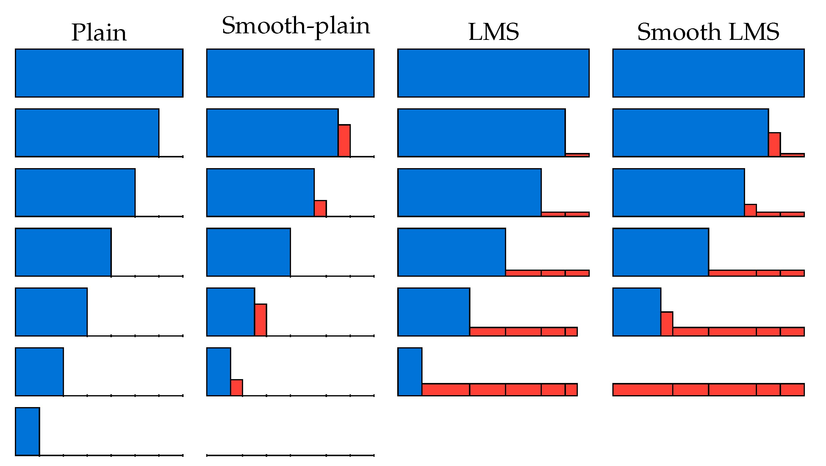
Figure 1.
An illustration of how the magnitudes of the vectors change over the reduction steps for different versions of the BKW algorithm. The heights correspond to magnitudes and the width corresponds to the number of positions. The figure is taken from [34].
Figure 1.
An illustration of how the magnitudes of the vectors change over the reduction steps for different versions of the BKW algorithm. The heights correspond to magnitudes and the width corresponds to the number of positions. The figure is taken from [34].


Table 1.
The comparison between and
| q | |||
|---|---|---|---|
| 1601 | |||
| 1601 | |||
| 1601 | |||
| 1601 |
Table 2.
Estimated time complexity comparison (in ) for solving LWE instances in the TU Darmstadt LWE challenge [29]. Here, an unlimited number of samples is assumed. The last columns show the complexity estimation from the LWE estimator [7]. “ENU” represents the enumeration cost model is employed and “Sieve” represents the sieving cost model is used. Bold-faced numbers are the smallest among the estimations with these different approaches.
| n | q | LWE Estimator [7] | ||||||||
|---|---|---|---|---|---|---|---|---|---|---|
| BKW- FWHT-SR | Coded- BKW | usvp | dec | dual | ||||||
| ENU | Sieve | ENU | Sieve | ENU | Sieve | |||||
| 40 | 1601 | 0.005 | 34.4 | 42.6 | 31.4 | 41.5 | 34.7 | 44.6 | 39.1 | 47.5 |
| 0.010 | 39.3 | 43.7 | 34.0 | 44.8 | 36.3 | 44.9 | 51.1 | 57.9 | ||
| 0.015 | 42.4 | 52.6 | 42.5 | 54.2 | 43.1 | 50.6 | 61.5 | 64.4 | ||
| 0.020 | 46.2 | 52.6 | - | - | 51.9 | 58.2 | 73.1 | 75.9 | ||
| 0.025 | 48.3 | 52.7 | - | - | 59.2 | 66.1 | 84.7 | 85.4 | ||
| 0.030 | 50.0 | 52.7 | - | - | 67.1 | 68.9 | 96.3 | 92.5 | ||
| 45 | 2027 | 0.005 | 37.7 | 55.2 | 31.8 | 41.9 | 35.0 | 44.8 | 41.5 | 51.6 |
| 0.010 | 43.5 | 55.2 | 39.5 | 51.2 | 41.2 | 48.2 | 57.0 | 64.6 | ||
| 0.015 | 48.3 | 55.2 | 50.4 | 61.3 | 51.2 | 58.3 | 74.3 | 74.9 | ||
| 0.020 | 51.2 | 55.2 | - | - | 61.1 | 65.0 | 86.8 | 86.1 | ||
| 0.025 | 54.1 | 55.3 | - | - | 71.0 | 71.4 | 100.7 | 95.0 | ||
| 0.030 | 56.3 | 64.1 | - | - | 80.2 | 78.7 | 116.2 | 104.1 | ||
| 50 | 2503 | 0.005 | 41.8 | 46.4 | 32.4 | 42.6 | 35.5 | 45.1 | 46.7 | 58.0 |
| 0.010 | 48.7 | 56.0 | 46.0 | 57.5 | 47.6 | 54.1 | 66.8 | 65.4 | ||
| 0.015 | 52.5 | 56.8 | - | - | 60.8 | 63.6 | 84.9 | 83.5 | ||
| 0.020 | 56.4 | 61.9 | - | - | 72.1 | 72.1 | 101.9 | 96.5 | ||
| 0.025 | 59.3 | 66.1 | - | - | 83.5 | 80.8 | 120.0 | 105.7 | ||
| 0.030 | 63.3 | 66.3 | - | - | 94.2 | 89.1 | 134.0 | 115.6 | ||
| 70 | 4903 | 0.005 | 58.3 | 62.3 | 52.3 | 54.2 | 55.2 | 63.3 | 76.2 | 75.9 |
| 0.010 | 67.1 | 73.7 | - | - | 80.4 | 77.1 | 111.3 | 98.9 | ||
| 0.015 | 73.3 | 75.6 | - | - | 102.5 | 93.2 | 146.0 | 118.0 | ||
| 120 | 14,401 | 0.005 | 100.1 | 110.5 | 133.0 | 93.2 | 135.5 | 111.4 | 181.9 | 133.2 |
| 0.010 | 115.1 | 124.0 | - | - | 195.0 | 150.4 | 266.2 | 165.7 | ||
| 0.015 | 127.0 | 136.8 | - | - | 246.4 | 183.2 | 334.0 | 209.8 | ||
Table 3.
Experimental results on target parameters. When using FBBL, parallelization was used only in the guessing phase, while the reduction phase was executed on a single core. M stands for millions, B for billions.
Table 3.
Experimental results on target parameters. When using FBBL, parallelization was used only in the guessing phase, while the reduction phase was executed on a single core. M stands for millions, B for billions.
| n | q | n. of Initial Samples | Running Time | Library | Machine | Cores | |
|---|---|---|---|---|---|---|---|
| 40 | 1601 | 0.005 | 16 M | 19 s | RBBL | B | 15 |
| 40 | 1601 | 0.005 | 16 M | 5 min 53 s | FBBL | B | 15 |
| 40 | 1601 | 0.005 | 16 M | 3 min 57 s | FBBL | A | 15 |
| 40 | 1601 | 0.010 | 570 M | 1 h 41 min | FBBL | A | 15 |
| 40 | 1601 | 0.015 | 4.2 B | 1 d 14 h | FBBL | A | 15 |
| 45 | 2027 | 0.005 | 250 M | 1 h 0 min | FBBL | A | 15 |
| 45 | 2027 | 0.010 | 8.3 B | 4 d 21.5 h | FBBL | A | 15 |
| 50 | 2503 | 0.005 | 2.7 B | 1 d 1.5 h | FBBL | A | 15 |
Publisher’s Note: MDPI stays neutral with regard to jurisdictional claims in published maps and institutional affiliations. |
© 2021 by the authors. Licensee MDPI, Basel, Switzerland. This article is an open access article distributed under the terms and conditions of the Creative Commons Attribution (CC BY) license (https://creativecommons.org/licenses/by/4.0/).
Share and Cite
MDPI and ACS Style
Budroni, A.; Guo, Q.; Johansson, T.; Mårtensson, E.; Wagner, P.S. Improvements on Making BKW Practical for Solving LWE. Cryptography 2021, 5, 31. https://0-doi-org.brum.beds.ac.uk/10.3390/cryptography5040031
AMA Style
Budroni A, Guo Q, Johansson T, Mårtensson E, Wagner PS. Improvements on Making BKW Practical for Solving LWE. Cryptography. 2021; 5(4):31. https://0-doi-org.brum.beds.ac.uk/10.3390/cryptography5040031
Chicago/Turabian StyleBudroni, Alessandro, Qian Guo, Thomas Johansson, Erik Mårtensson, and Paul Stankovski Wagner. 2021. "Improvements on Making BKW Practical for Solving LWE" Cryptography 5, no. 4: 31. https://0-doi-org.brum.beds.ac.uk/10.3390/cryptography5040031