Tools to Ease the Choice and Design of Protein Crystallisation Experiments

Abstract

The process of macromolecular crystallisation almost always begins by setting up crystallisation trials using commercial or other premade screens, followed by cycles of optimisation where the crystallisation cocktails are focused towards a particular small region of chemical space. The screening process is relatively straightforward, but still requires an understanding of the plethora of commercially available screens. Optimisation is complicated by requiring both the design and preparation of the appropriate secondary screens. Software has been developed in the C3 lab to aid the process of choosing initial screens, to analyse the results of the initial trials, and to design and describe how to prepare optimisation screens.

1. Introduction

There are a number of techniques which can produce atomic resolution structures of macromolecules (for example, proteins), but by the far the most productive technique to date is X-ray crystallography [1], whereby a crystal of the sample of interest is irradiated with high-energy X-rays, and the resultant diffraction pattern deconvoluted to give an image of the molecules making up the crystalline sample [2]. The production of ‘diffraction quality’ crystals is required for the generation of atomic resolution structures by X-ray crystallography, and this is the major limitation of the technique [3].

Although there are many techniques used for growing crystals [4], most crystals are grown using the method of vapour diffusion, in which a droplet of pure, concentrated protein is mixed with a droplet of a chemical mixture (also called the condition, or the cocktail), and the combined droplet is allowed to equilibrate against a larger volume of the cocktail. These experiments can be hanging drop experiments (often set up laboriously by hand, in 24 well arrays) or sitting drop experiments (which are more likely to be set up with the help of automation, in 96 well arrays). The screening experiments most often use standard sets of conditions, ‘commercial screens’ which are widely available through a number of different vendors. Many different commercial screens exist. The variables for the screening step are quite limited—what screen(s) to use, what protein concentration to test, how much of the protein sample to include in the experimental drop, how much of the condition to include (i.e., the ratio of these two liquids), and the temperature at which to incubate the experiments. Each experimental droplet must be examined, over a number of days or weeks for indications of a crystalline outcome. If a suitable crystal is observed it can be harvested from the screening droplet, but most often several cycles of optimisation are needed before a suitable crystal is obtained.

Optimisation can be done in many different ways [5], but almost all optimisation requires the design and creation of a focused screen around conditions that appear to be promising from the initial screening. This might be a screen using only chemicals found in ‘hits’ from the screening (often called fine screening), or it might be a single cocktail, which is dispensed 96 times and where each well is tweaked by the addition of a different chemical (additive screening). Optimisation requires more decision making than screening, even putting aside the often very difficult question of what screening condition(s) should be included in subsequent optimisation. Each cocktail consists of one or more chemical factors, that is, a chemical with an associated concentration, concentration unit and possibly pH value. In optimisation fine screening, one has to choose which chemicals to include, what concentration, or concentration range, to use for each chemical, and possibly which pH or range of pH values to be tested. On top of this there are orthogonal considerations that interfere with the design process, such as the solubility and/or buffering range of a chemical, or the possibility of unwanted interactions. For example, mixing solutions of calcium chloride and ammonium sulfate, two commonly used chemicals in protein crystallisation, will inevitably lead to the formation of calcium sulfate crystals, confounding the interpretation of the optimisation outcome.

There are a number of applications that estimate the likelihood of a successful protein crystallisation given a sequence [6,7,8,9,10], but there are few software tools available that help to clarify what to actually do in the laboratory to make the protein crystallise. A common approach is to do a search to see if the target of interest has been crystallised before, and use the published conditions as a starting point. If the target of interest has not been crystallised, then often the advice is to search for (and then start screening with) crystallisation conditions used to crystallise similar proteins (perhaps in the Biological Macromolecule Crystallization Database (BMCD; http://bmcd.ibbr.umd.edu/)) [11], although recently the soundness of that approach has been questioned [12]. However, even if the protein target has been crystallised previously, the literature conditions tend only to be a rough guide—subtle differences in the exact construct and/or expression and purification can alter how the protein target behaves in crystallisation experiments. Nevertheless, published conditions can narrow down the screening process—for example, by suggesting that trialling conditions containing mid-range polyethylene glycol (PEG) might be appropriate.

The Collaborative Crystallisation Centre (C3; http://crystal.csiro.au/) is a full service protein crystallisation facility operated by the Commonwealth Scientific and Industrial Research Organisation (CSIRO) in Parkville, Australia. It was set up in the early 2000s to give the local structural biology community access to crystallisation automation, but has extended its mandate since then to provide novel software tools to facilitate the process of growing macromolecular crystals. To make the software tools accessible, the tools are web-based, and include manuals on how to use the various features of the programs. This report aims to give an flavour of what the tools can do, rather than describe in detail how each feature works.

One of the first software tools developed in the C3 was the C6 webtool [13]. C6 (https://c6.csiro.au/) was designed over ten years ago to provide a tool that would answer questions such as ‘Which commercial screen contains the most PEG 8000?’, or ‘What range of ammonium sulfate concentrations are found in Crystal Screen HT from Hampton Research?’ The web server PICKScreens [14] (https://registration.cc.biophys.mpg.de/pickscreens/) had a similar mandate. The C6 tool tries to capture information about all the commercial screens in a format to allow these types of queries. Of course, some of this information could be found by navigating to each vendor’s website in turn, but the advantage of the C6 tool was the translation of all of the screen information provided by the vendor into a common vocabulary [15], which enabled the development of a heuristic distance measurement between individual conditions and screens [13]. Formalising the concept of similarity has been found useful by other groups since as well [16]. There were 220 commercial screens captured in the original C6 tool (compared to the 129 in the PICKScreens database), since then over 100 new commercial screens have been added. A further function of the original C6 tool was to provide a list of what screens were physically present in C3, and thus available for use by the C3 user community. Along with new commercial screens, other features and improvements have been added to the original tool. The most fundamental was a ≈1000× increase in the speed of generating the underlying database, with a concomitant increase in the real time utility of the tool. In this paper we describe five of the more novel/useful new features of the C6 program.

More recently, we have developed a viewing, scoring and optimisation tool ‘See3’. See3 (https://see3.csiro.au/) incorporates a machine learning (ML) tool (MARCO) [17] which runs in real time and returns one of four possible classifications to images of the crystal experiment (Clear, Precipitate, Crystal or Other). The MARCO tool was generated using a multi-layered neural network (deep learning) using a large set of training images of ≈500,000 human scored collected from a consortium of academic and industrial crystallisation groups. The generated classification is estimated to be about 90% accurate for the images collected in C3. The MARCO scores, along with manual human scoring, can be used to generate fine screens for optimisation.

Overview of the C6 and See3 Programs

The See3 program is a web-based application for the viewing, scoring and optimisation of crystallisation experiments which have been set up within C3. The C6 program is a tool for the analysis and comparison of crystallisation screens, both those commercially available and those designed in the See3 application. The two applications both rely on information from the ‘CM’ crystallisation database in C3. This is an Oracle™12c database, which started as the ‘Crystal’ database provided by the (now defunct) company RoboDesign (then Rigaku) with their Minstrel imaging system. Although C3 migrated from the Minstrel imagers in 2016, C3 continues to use the CM database, thus preserving ten years of legacy data, and uses a Dynamic-link library (DLL) to translate between the CM schema and the dataforms required to run the current (Formulatrix RI-1000) imagers. The CM database captures information about the screens (and the cocktails that make up the screens), samples, users, images, scores, as well as tracking the barcoded deepwell blocks and experimental crystallisation plates used in C3. Both See3 and C6 have public information (commercial screens and screens offered by C3) and private information (any data associated with a particular user). The latter is password protected and only visible to the authorised users.

2. C6

The C6 program is a webtool which catalogues and compares crystallisation conditions. The tool contains (most of) the commercial crystallisation screens, along with screens designed by users of the C3 crystallisation facility. The data in the C6 SQLite database is derived from the screen information in the CM database; along with the chemical description of each cocktail in every screen obtained from the CM database, the C6 database contains a matrix of distances between every pair of crystallisation cocktails [13]. The matrix of distances allows the calculation of screen (dis)similarity. This, for example, allows for the trivial identification of commercial screens which are essentially the same, which is hard to do by hand, as each vendor may have the same set of conditions in a screen, but ordered (or even spelled) differently (Figure 1).

As in the earlier version [13], each screen in C6 can be displayed as a set of cocktails, or as a list of the component chemicals, with usage count, concentration and pH ranges. The interface has been updated, and now groups the available reports into logical classes. Under each section one can choose from a predefined subset of all screens, e.g., ‘C3 screens’, or ‘Commercial Screens from Hampton Research’. C6 also allows for the creation of both persistent custom subsets or on-the-fly custom subsets of screens.

Within each section the queries can be filtered by subsets of screens, such as only those screens available within C3, or only those screens sold by the vendor Hampton Research. For example, if one wanted to see which screens are currently available from Molecular Dimensions, one would select the report ‘Screens Lists’, and choose the filter ‘Commercial Screens’, then the filter ‘Molecular Dimensions’.

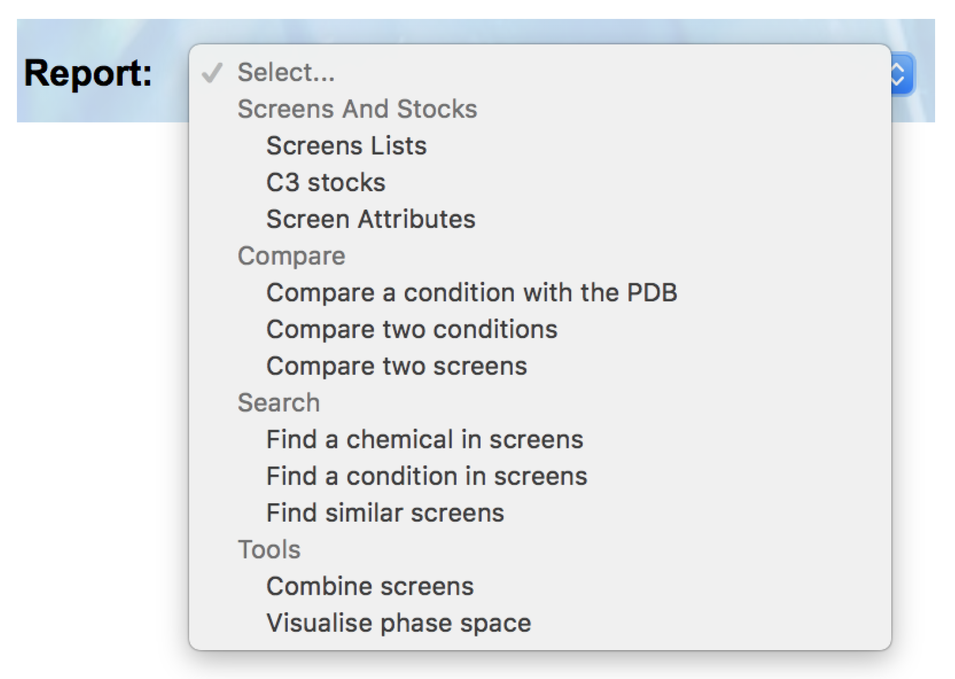
2.1. Interface

C6 now breaks down the available reports into four sections: ‘Screens and Stocks’, ‘Compare’, ‘Search’ and ‘Tools’ (Figure 2).

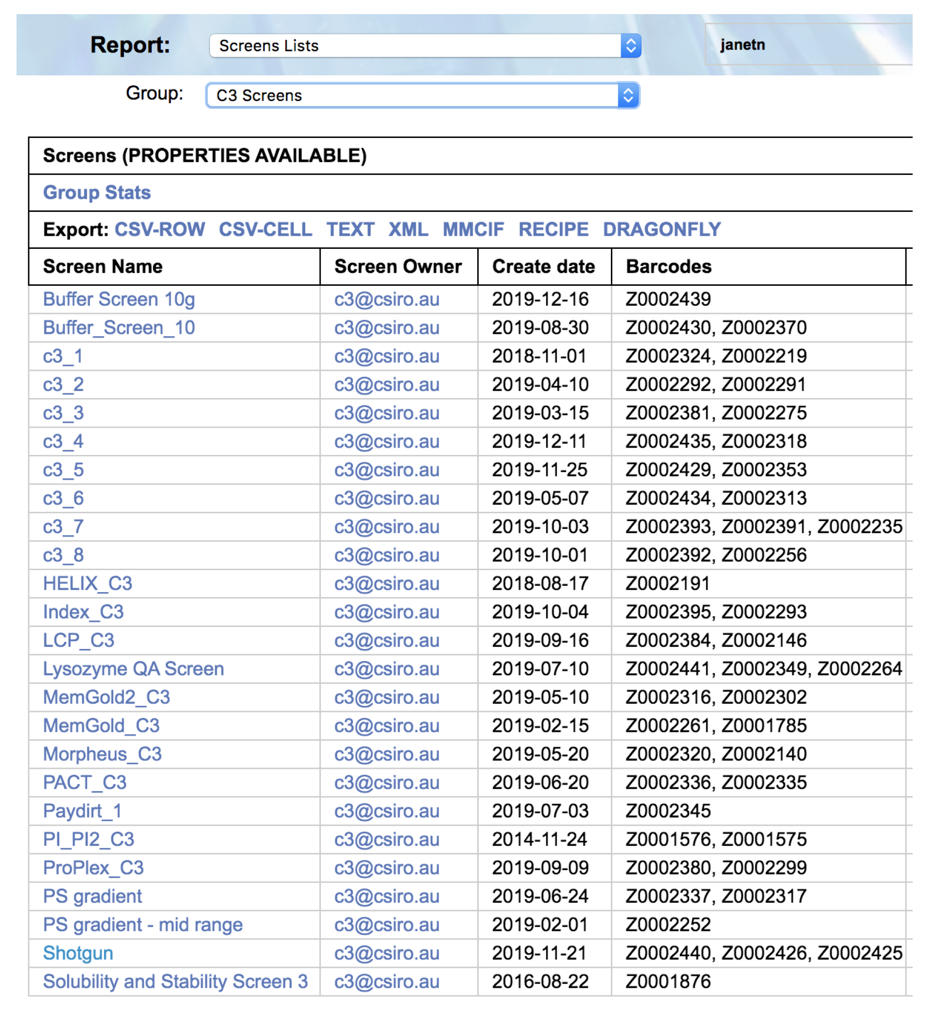
Once the appropriate filters have been selected a list of screens is returned. Each screen name is selectable, and clicking on a screen name will open a new browser tab containing a header containing information about the screen, followed by a listing of the contents of each well of the screen (Figure 3).

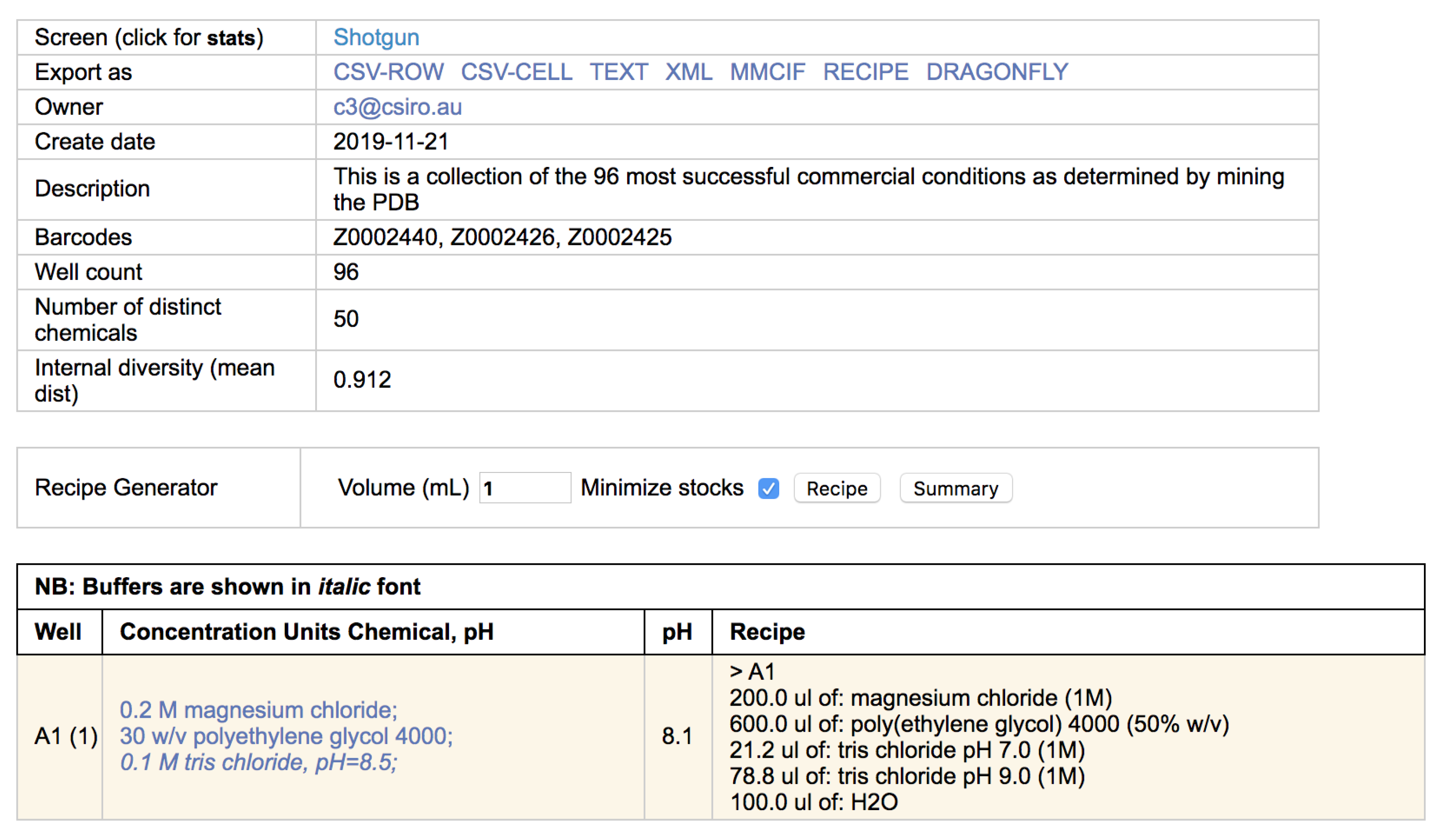
Clicking on the screen name will open up a new browser tab containing a listing of the chemicals found in each well. If the cocktail can be made with C3 stocks (i.e., the chemicals are named appropriately, and C3 has stocks of appropriate concentration and/or pH) then a recipe of how that condition can be made is also provided (Figure 4).

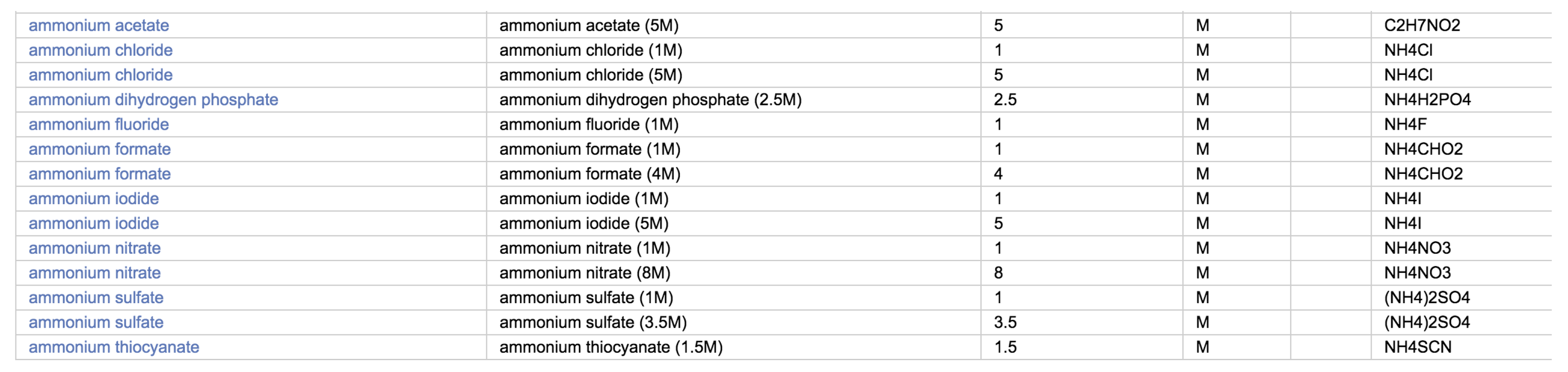
The report ‘C3 Stocks’ found under the section ‘Screens and Stocks’ gives a listing of all the stocks currently available in C3 (Figure 5).

Another new feature of the interface is the inclusion of an updated User Manual and Frequently Asked Questions (FAQ) list, but more importantly, there are inbuilt tools that support the facile generation of new entries into the FAQ list. The landing page of the C6 tool, like most of the outward facing web-tools from C3 includes a Twitter feed, where tweets from the C3 Twitter account (@CSIROC3) are displayed. This provides a mechanism for notifications in real time.

2.2. Screen Attributes

One of the screen metrics that was available in the original C6 was the concept of “Internal Diversity” (ID). This is a global measure of how different each condition in a screen is from the other conditions in the same screen. ID is normalised to give a value between 0 and 1; screens with an ID of 0 have each condition in the screen identical to the others, screens with an ID of 1 consist of conditions with no common chemicals in them. The ID value of a screen can be used to identify what type of screen it is, and thus where to use it in a crystallisation campaign. Screens with low ID (<0.5) are often grid screens, or screens with few chemicals in them; these screens are most often optimisation tools (fine screens) and are used once initial conditions have been identified. Screens with very high ID (≈1) are most likely to be additive screens; these are used in the early stages of optimisation. Screens with a high ID (≈0.9) are often the initial “sparse matrix” [19] screens and are used at the start of a crystallisation project. Other useful global features of a screen might be the pH range it samples, or the relative amount of salty or PEG-based conditions it contains. All these global indicators are available through the Screens Attribute report. This report returns a sortable table, as shown in Figure 6.

2.3. Persistent Screen Sets

Many of the C6 reports require the selection of a subset of screens on which to perform the report action. For example, when using either the ‘Find a chemical in screens’ or ‘Find a condition in screens’ report, the user is prompted to select a pre-defined subset of screens, such as ‘C3 screens’ or ‘Commercial screens’ in which to search for the chemical (or condition). Initially C6 only offered pre-defined screen subsets, and although these pre-defined sets were helpful, there are cases where the user might wish to choose their own subset of screens. Being able to define one’s own specific subset of screens is particularly useful for users outside the C3 user community, who can create a subset of commercial screens corresponding to those they have in their home laboratory. The creation of screen sets is done through the report ‘Create a set of screens’, found in the ‘Tools’ section of the top menu. The user-defined sets persist in the C6 database and can be edited as needed. Any user-defined screen sets are found under the ‘My Screen Sets’ filter option (Figure 7).

The screens able to be added to a user’s screen set include all private screens belonging to the user, and all public screens both commercial and in-house (C3 screens). These are presented in a list, and can be searched via the search bar for ease of use. From the same report, existing screen sets can be modified or deleted as well as created, and all changes take effect immediately and will update accordingly in the screen group selection boxes in the other C6 reports.

2.4. Recipes

Most often a crystallisation screen is described as a set of conditions, where each condition contains one or more chemical factors. This way of documenting a screen does not capture how the condition was made—for example, 1 mL of a simple condition containing only 1 M sodium chloride could be made by pipetting out 1 mL of a 1 M sodium chloride stock, or by pipetting out 0.2 mL of a 5 M sodium chloride stock and adding 0.8 mL water. Generally, we refer to the description of a crystallisation condition in terms of concentration as a ‘design’ and the description of the the same solution in terms of stocks and volumes as a ‘recipe’. For every condition that can be created with C3 stocks the recipe for producing 1 mL of that condition is given alongside the design of that condition (see Figure 4). If every condition in the screen can be created with the stocks available in C3 then an option appears in the header of that screen to export a file containing the recipes for every well. The final volume required can be stipulated (it defaults to 1 mL), and the recipe can be exported in different formats. To date the export formats include an xml format and a human-readable csv format suitable for import into the Dragonfly (SPT Labtech) liquid dispensing robot (Figure 8).

2.5. Phase Space Visualisation

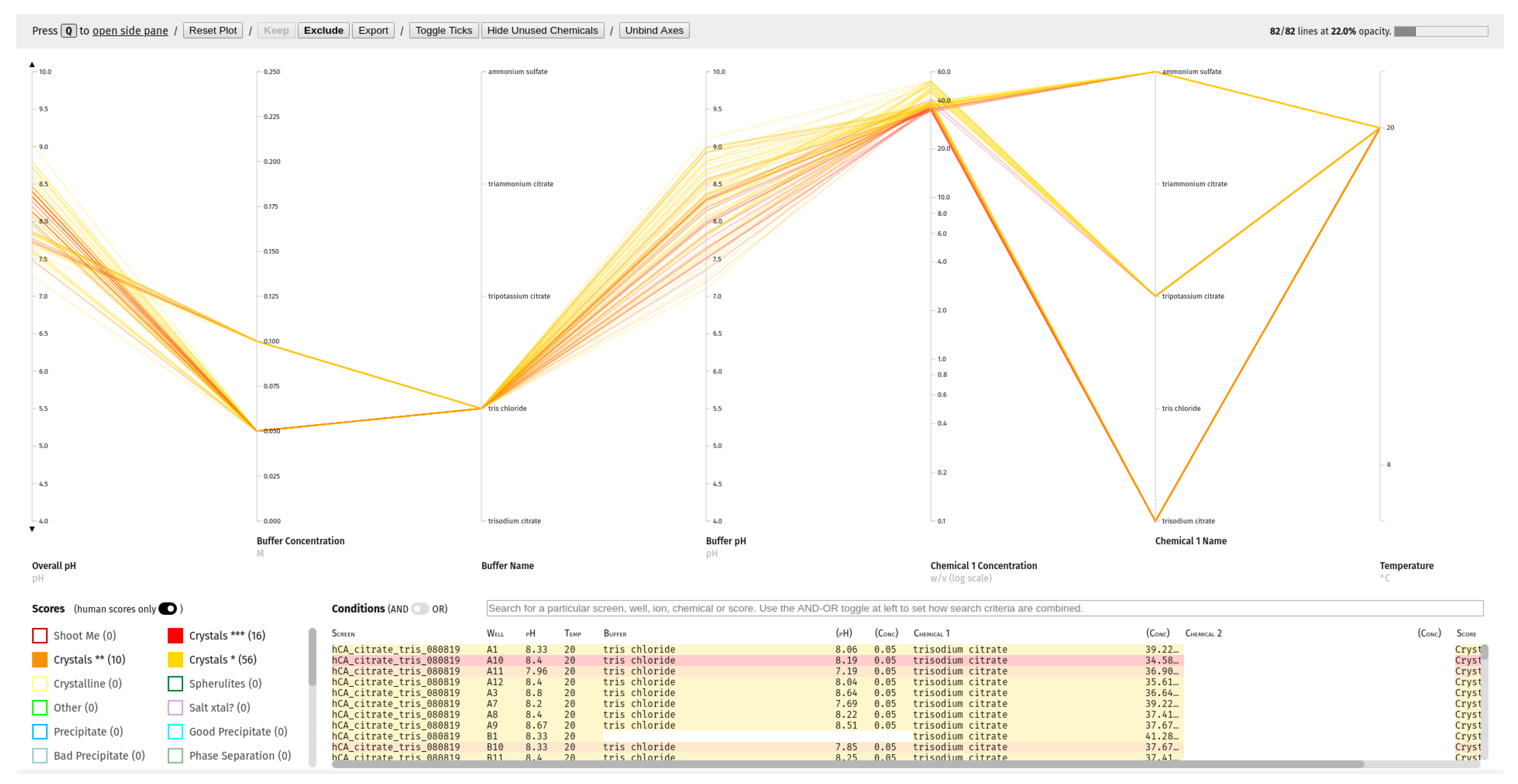
Both fine screening and additive screening methods of optimisation rely on the user having a clear understanding of patterns in the outcomes of previous crystallisation experiments. In practice, such understanding is often sought by unsystematically eyeing a table of conditions in the hope of spotting commonalities between successful experiments. With this approach, one is prone to missing important positive correlations between a particular condition and the formation of crystals, or conversely, not grasping which areas in the condition space have been explored thoroughly without proving fruitful. While progress is being made towards automation of this analysis using chemical ontologies, human expertise will continue to be valuable, so there is a need for tools that augment human abilities to perceive which points in condition space have been tested for a given protein, and what the outcomes of those experiments were.

To this end, a ‘Visualise phase space’ report has been added to C6, which, for any user-selected combination of experiment barcodes, plots a subset of the conditions used including temperature, pH, chemical species and concentration on an interactive parallel coordinates plot (a common plot-type for high-dimensional data). Each experiment is represented by a line intersecting each of the condition axes at the relevant value, and the colour of each line indicates the outcome of the experiment it represents (as scored by the user in See3). Axes can be reordered, inverted or removed to make key trends clearer. Experiments can be easily filtered by any of the axis dimensions, as well as screen, well or outcome. To aid new users, a draggable card summarising the available interactions can be displayed on top of the interface, which also links to a video walk-through of how to use it.

An example plot is included in Figure 9.

3. See3

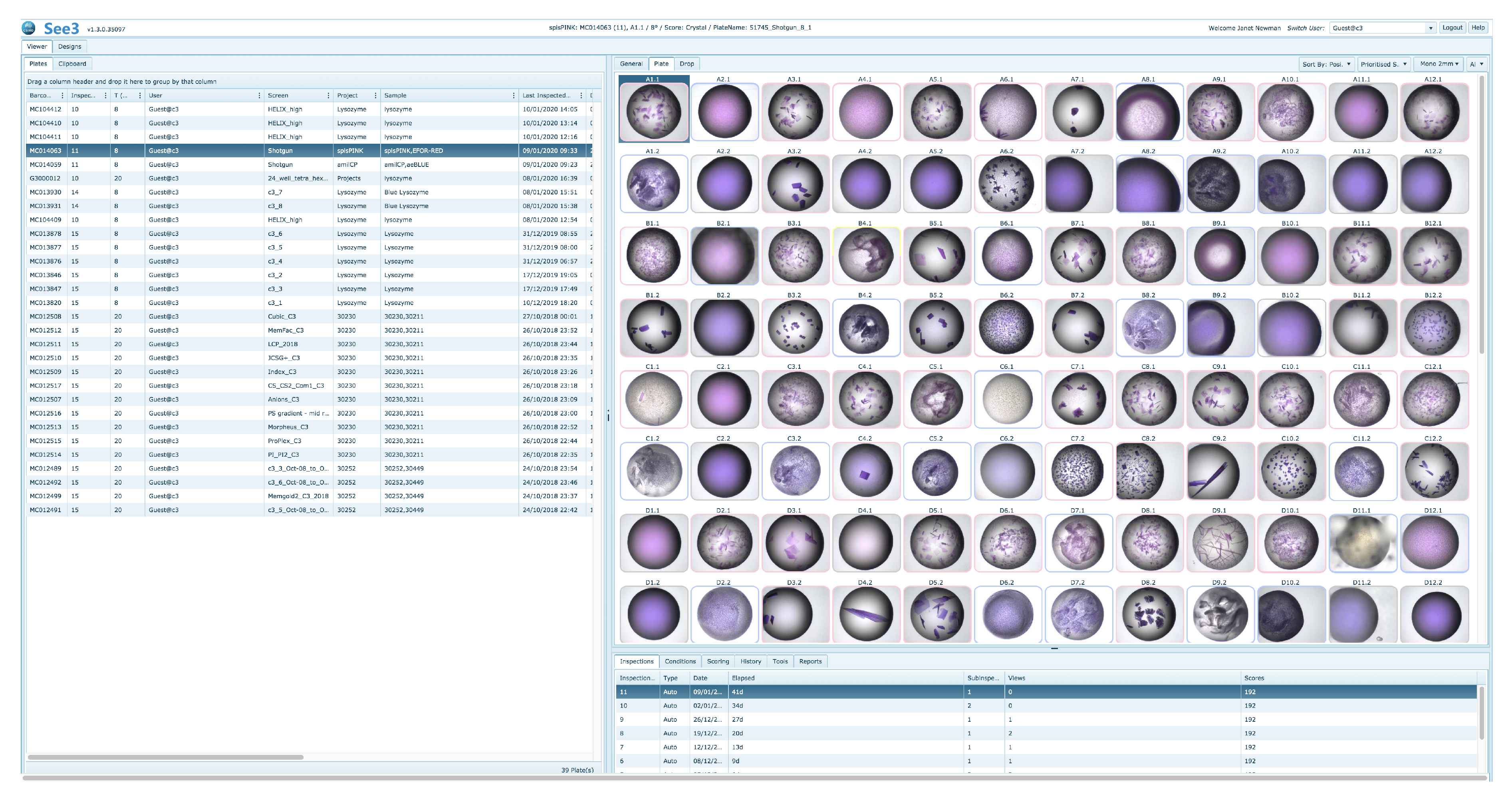
See3 has three major sections—a viewing and scoring section, a design section and an administration section, which is not visible to the general user. The viewing and design sections are accessible to all users; a user will see only plates owned by themselves. The viewing and scoring section of See3 provides the user with a selection grid of existing crystallisation plates. After a plate is selected See3 shows a grid of the most recent images associated with that plate (Figure 10).

By default, the thumbnail images are arrayed in a grid corresponding to their position on the crystallisation plate, however the images may also be arrayed by scores. A MARCO autoscore for each image is generated automatically and associated with an image, and human scores can also be associated with each image. A visual indication of the score for a well is given in the coloured border around the well [20]. Sorting by score will display images with Crystal scores first, followed by images with Other scores, then Precipitate scores and finally those with Clear scores, with human scores in each category being shown before autoscored images with the same classification. Double-clicking on a thumbnail will open up a larger image, and display associated information, including the sample name, the cocktail name, and what chemicals they respectively contain.

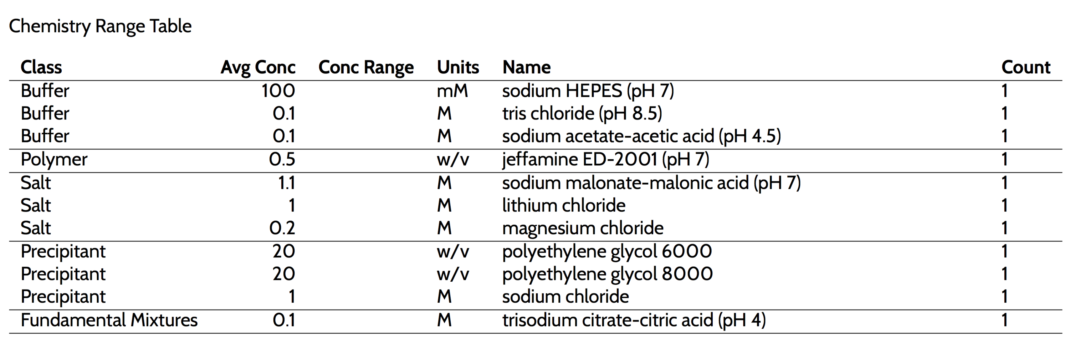
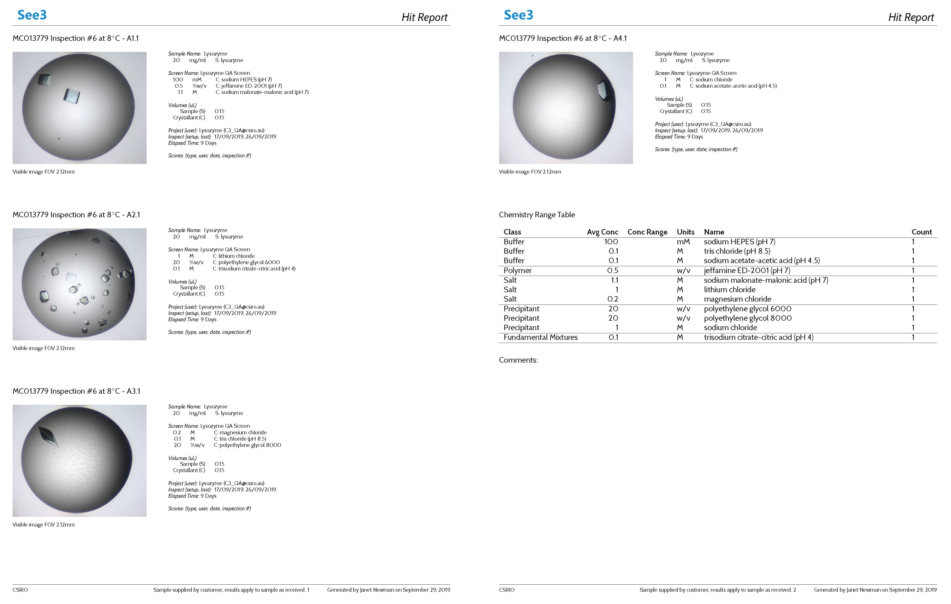
Users may place images from one or more plates on to a clipboard, this is a way of cherry-picking conditions for cycles of optimisation. The images on the clipboard can be used to generate a hit report (see Supplementary Information for an example of a hit report for a crystallisation plate set up with the protein Lysozyme). The hit report contains the details of conditions and samples in the droplets contained in the images, listed for each image on the clipboard. The hit report concludes with a summary of the chemical factors (the ‘Chemistry Range Table’) found in the conditions on the clipboard (Figure 11).

If appropriate images were placed on the clipboard, the information in the ‘Chemistry Range Table’ is a reasonable starting point for optimisation through fine screening. The optimisation tool allows one to work with the information from the clipboard to design new screens. Once designed and saved, the screens will appear in the next build of C6, generally within an hour. By default, the nascent design in See3 is checked against the stocks available in C3 before being saved, thus any design that was saved successfully in See3 will be able to be produced with C3 stocks, and the recipe for its creation will be available from C6, along with the screen description.

4. Features in See3

The See3 application initially provided a modern viewing, scoring and reporting tool for images collected in C3. Many of the features included in the viewing component of See3 are standard, and are found in many viewing programs—for example, measuring tools, drop history, drop components etc. Along with the expected functions, See3 has some tools which were built after user feedback. These include a tool for adjusting the zoom or centre of images, the ability to see the recipe for a single condition and the ability to select and write out regions of interest within crystallisation images. Beyond the viewing capability, See3 allows users to design optimisation experiments. Optimisation screens can be automatically generated from information on the clipboard, or can be created from a blank slate by the user. Screens can be in 24, 48 or 96 well formats.

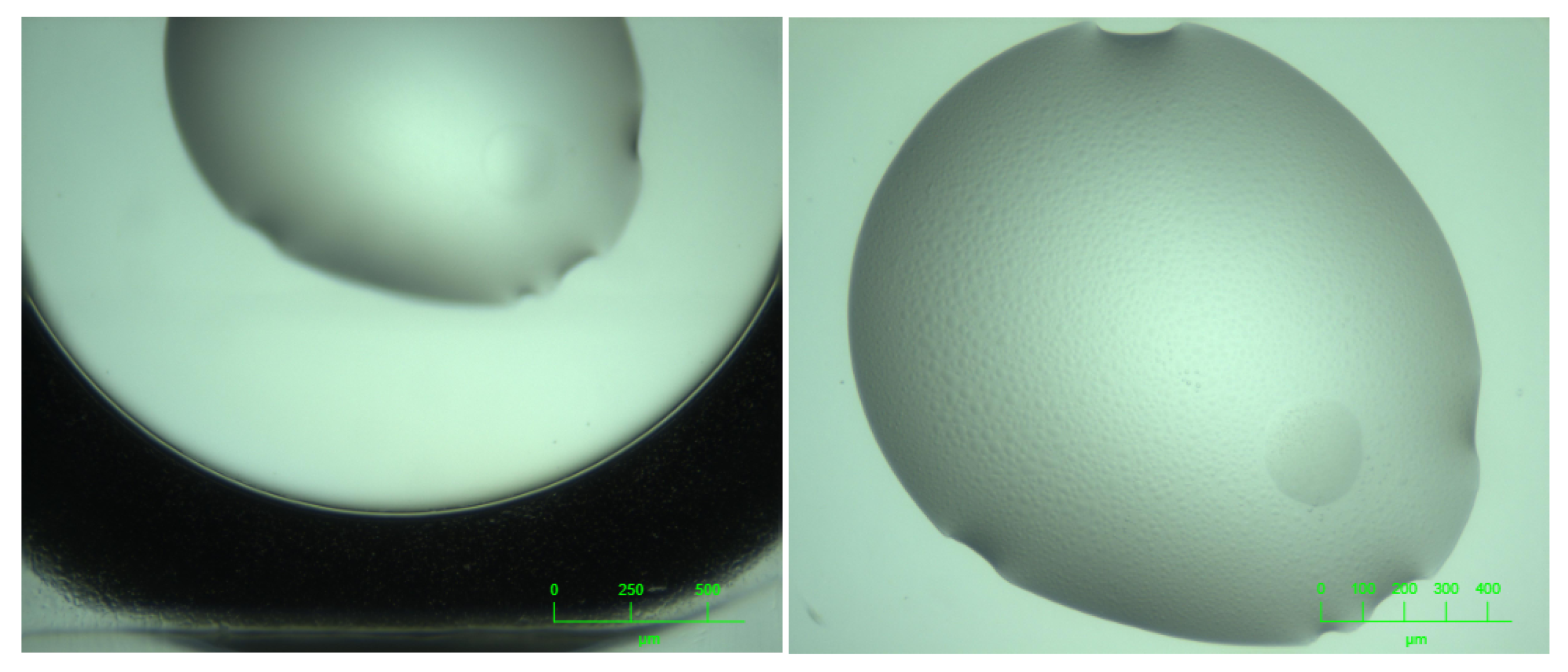
4.1. Recentering Images

The very first image of a drop is at a zoom level that encompasses the entire subwell in which the droplet is located. This image is segmented by the RockImager software and subsequent images are taken at a zoom level and with centre coordinates so that the experimental droplet fills the field of view. Mostly this process works well, but it fails sufficiently often that a tool that allows the user to reset the centre and zoom level (to be used on the subsequent images of that droplet) has proven very useful (Figure 12).

4.2. ROI Setting and Export

Being able to locate a subregion within a droplet can be used for a number of purposes: to earmark particular crystals for harvesting, or for in-situ X-ray interrogation. Within the See3 viewing software one can mark one or more regions of interest (ROI), and the coordinates of these can be exported. The $(x,y)$ coordinates of the ROI are relative to the centre of the subwell. A Z-offset is also included which gives the curved surface depth of the subwell (assuming the plate is an MRC sitting drop plate) at the ROI position.

4.3. Optimisation

Optimisation is the refinement of initial screening conditions with the goal of producing a well diffracting crystal. Aside from microseeding [21], the most common methods of optimisation are fine screening, using information gleaned from any previous experiments, and additive screening, where a single promising condition is doped with many different chemicals to test their effect on the crystallisation process. The optimisation function of See3 has two distinct modes for optimisation; an Automatic and a Manual mode. In essence, the Automatic mode considers the entire screen as a entity, whereas the Manual mode considers the individual wells as components that together make up a screen.

4.3.1. Automatic Optimisation

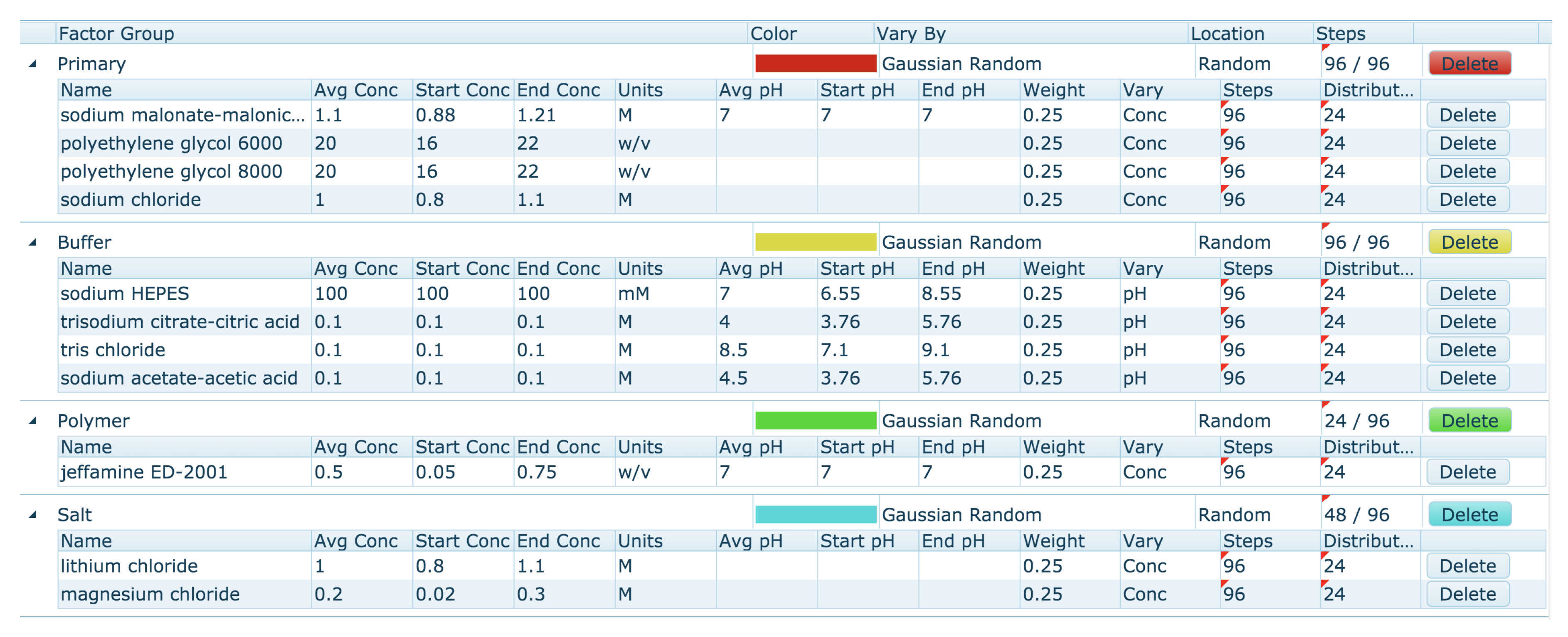
The Automatic optimisation tool allows the generation of a new optimisation screen based on the currently selected conditions on the clipboard. By default, the Automatic mode generates a screen by populating each well with a random pick of a chemical from a number of Factor Groups, and assigns a random concentration (from a range) for each chemical. The first step is the clustering of the chemicals found on the clipboard into Chemical Factor groups. This grouping of chemicals is based on their class or role, and is similar to how the chemicals are grouped in the ‘Chemistry Range Table’ (Figure 11). The Primary Factor Group contains the chemicals that are found at the highest concentration in each of the conditions selected on the clipboard. Other default Chemical Factor Groups include Buffers, Polymers, Organics and Salts. Each chemical within a Factor Group is given four attributes: a flag which decides if the concentration or the pH is to be varied (conc/pH flag), a lower limit, an upper limit, and a weight. The attributes are set from the values seen in the ‘Chemical Range Table.’ For chemicals with the pH/conc flag set to ‘conc,’ the upper and lower values are set according to the average concentration of that chemical found in the ‘Chemical Range Table.’ For chemicals in the Primary Factor group (and for chemicals found at greater than 0.5 M), the default limits are $0.8\times$ average concentration for the lower limit, and $1.1\times$ average concentration for the upper limit. For other Factor groups the concentration limits are $0.1\times$ average concentration (lower limit) and $2\times$ average concentration (upper limit). The pH range is set by default to the (nearest) pK_a for the buffer $\pm 1$ pH unit. The weight of the chemical depends on how many clipboard conditions contained that chemical. The Factor Groups for the ‘Chemical Range Table’ shown in Figure 11 are shown in Figure 13.

The weighting and upper and lower limits can be edited, chemicals can be added or deleted from Factor groups, and Factor Groups can be added or deleted. Users also have some control over where different chemicals can be found on the plate, and how the concentration or pH values are chosen. The user can choose to include the original hit conditions (those placed on the clipboard) in the final design. The screen generated from the Factor Group table can be saved, also the Factor Group table can be saved. Of course, if a saved Factor Group is re-loaded, it is unlikely that exactly the same screen will be generated again, due to the random selection of concentrations.

After the optimisation screen has been generated, it undergoes a number of checks before it can be saved. If the screen cannot be created with C3 stocks it will not be saved, and the user will be alerted. The most common reason for failing to save is that the available stocks are not sufficiently concentrated to make up the conditions. This is called ‘overflowing.’ If there are fewer than 20 overflowing wells, the program will try to correct this by reducing the concentration of the chemical from the Primary Factor group. The user will also be warned if incompatibilities such as divalent metals in the same condition as a phosphate salt are detected, but the incompatibility warnings do not preclude the screen from being saved.

4.3.2. Manual Optimisation

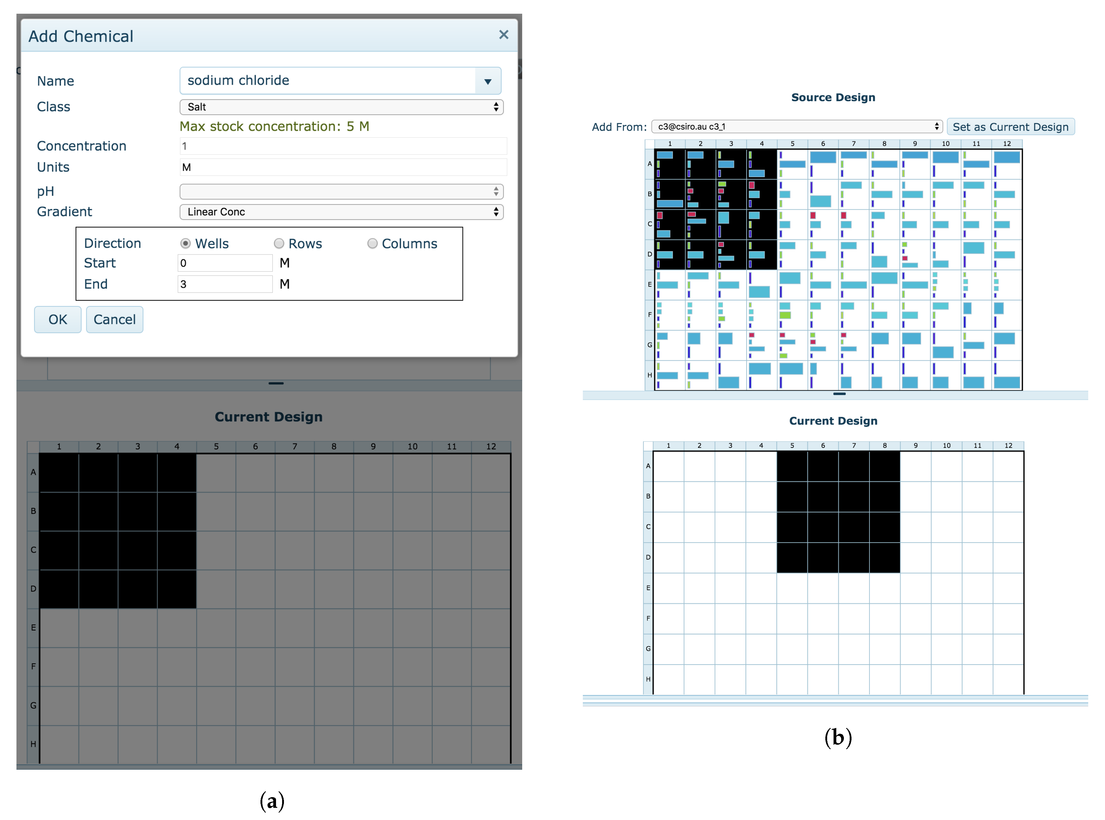
The Manual optimisation tool also enables the creation of a new optimisation screen but with greater customisability. Users are given a blank design and are free to create the experiment as they wish. Portions of existing designs or clipboard conditions can be copied, sections of the optimisation design can be repeated, individual chemicals can be added modified or removed, and chemical gradients can be placed across the new design (Figure 14).

When switching from the Automatic design to the Manual design, users are asked if they wish to begin their Manual optimisation design with their current Automatic optimisation design. This allows for the modification of specific conditions within an automatically generated screen.

5. Discussion

In the heyday of the Structural Genomics initiatives it was believed that simply by having sufficient protein, automation and appropriate screens any desired crystal—and thus structure—could be generated. More recent analyses suggest that screening alone is insufficient in about 80% of cases [22]. Once the truism that optimisation is required is accepted, then the pathway of crystallisation becomes less obvious. Which screens are best? What is a hit? Which conditions gave hits? How do I optimise the hit(s)? What is noticeably lacking is a set of tools to guide a structural biologist through this complicated process. We require tools for helping select initial screens, and for analysing the outcomes of those screens. Following that, tools are needed both to create designs for optimisation screens as well as to produce the recipes for those designs. Of course automation aids the process by enabling plate preparation, plate imaging and the production of screens. However, automation does not provide an answer to the question of what to do; without tools to help the researcher decide what is the best (or at least a reasonable) way forward, automation just speeds up the process of doing the wrong thing.

Our experience from working in a crystallisation core facility for over a decade suggests that one of the notable benefits of a facility is the expertise that builds up within the centre which then becomes available to the users of the facility. Most of the individuals using a crystallisation facility only spend a small percentage of their time thinking about crystallisation, as structure is only part of a bigger picture for understanding any protein system. Almost invariably, the users ask questions about what screens to use, “if this is a hit,” and then how to optimise. The development of the software tools described here is a result of our interactions with users, and is an effort to distill our experience so that it persists and can be shared. In particular, the hope that screening would solve the problem of crystal production has led to an explosion in the number of screens available. Counter-intuitively, this has made it harder to work out where to start.

The C6 tool cannot give answers about what is the ‘best’ screen with which to start a crystallisation campaign. However, given some information about the protein (e.g., it has been crystallised before in PEG) it can help select which screens to use. Further, C6 allows one to see if a further screen is testing a novel area of chemical space or is replicating conditions that have already been set up, and allows one to check a group of screens for condition redundancy. The visualisation tool provides an interactive interface for building up hypotheses about what parts of crystallisation space might be used to produce crystals, which can either guide subsequent screen selection or optimisation strategies.

The See3 viewing platform, coupled with reliable, real-time autoscoring, enormously speeds up the process of analysing the results of crystallisation trials. The link between finding a hit and creating optimisation from any hit(s) is aided by the automatic extraction of chemical factors from the hits. See3 optimisation tools are intuitive, and sufficiently sophisticated to allow for the design of almost anything that can be set up with current automation. The combination of automatic and manual screening modes brings the power of combinatorial optimisation which allows for the simultaneous optimisation of many conditions, with the specificity that comes from having control over each well. The most practical aspect of the optimisation is tying it in with stock availability, so that only screens which can be easily created can be designed.

Most importantly, these tools are web-based, and are available to the wider structural biology community. Both C6 and See3 can be accessed with a guest account (username guest@c3, password vegemite), or by registering as a C3 user. Any screens developed in See3 as a guest will be visible and editable by any other guest user, screens designed by a C3 user are only accessible by that user.

6. Materials and Methods

6.1. C6 Implementation

The C6 back-end was predominantly written in Python 2, which has now been migrated to Python 3, while the front-end is written in HTML/CSS and JavaScript. The similarity calculation comparison code has been implemented in C. C6 uses an internal SQLite database (https://www.sqlite.org/), which currently takes two days or so to build from scratch (pairwise comparisons of all screens), and roughly 7 minutes to update hourly, once initially built. The interactive data visualisation in the ‘Visualise Phase Space’ C6 report uses v3.5.17 of the d3.js JavaScript visualisation library (https://d3js.org/), with additional use of the jQuery library (http://jquery.com/) for various UI elements and keyboard shortcuts.

6.2. See3 Implementation

See3 is written as an ASP MVC.NET Framework project which is written with HTML/CSS and JavaScript for the front-end user interface, and C# for the back-end. The front-end JavaScript user interface is written using the Kendo UI framework. Back-end database connections to the Oracle CM database were written using the the Nhibernate framework.

6.3. MARCO Implementation

The MARCO autoscoring pipeline (C4) consists of a number of steps, and is controlled using a Python script, for a complete description see [23]. Briefly, Cron is used to provide lists of recently inspected plates; images from these are copied to a GPU cluster using scp. Images in batches of 32 are passed through a SLURM workflow manager where they are processed through the MARCO tensorflow AI. The output from this is post-processed to extract the single most likely classification and returned via SQL into the CM database. The C4 workflow is available from https://0-doi-org.brum.beds.ac.uk/10.4225/08/5a97375e6c0aa.