Article

Triple Solutions and Stability Analysis of Micropolar Fluid Flow on an Exponentially Shrinking Surface

1
School of Quantitative Sciences, Universiti Utara Malaysia, Sintok 06010, Kedah, Malaysia
2
KCAET Khairpur Mir’s, Sindh Agriculture University, Tandojam Sindh 70060, Pakistan
3
Faculty of Mathematics and Statistics, Ton Duc Thang University, Ho Chi Minh City 72915, Vietnam
4
Department of Mathematics, Cankaya University, 06790 Ankara, Turkey
5
Institute of Space Sciences, 077125 Magurele, Romania
6
Department of Medical Research, China Medical University Hospital, China Medical University, Taichung 40447, Taiwan
7
Department of Mathematics, College of Arts and Sciences, Prince Sattam bin Abdulaziz University, Wadi Aldawaser 11991, Saudi Arabia
*
Author to whom correspondence should be addressed.
Submission received: 11 March 2020 / Revised: 26 March 2020 / Accepted: 27 March 2020 / Published: 9 April 2020

Abstract

:
In this article, we reconsidered the problem of Aurangzaib et al., and reproduced the results for triple solutions. The system of governing equations has been transformed into the system of non-linear ordinary differential equations (ODEs) by using exponential similarity transformation. The system of ODEs is reduced to initial value problems (IVPs) by employing the shooting method before solving IVPs by the Runge Kutta method. The results reveal that there are ranges of multiple solutions, triple solutions, and a single solution. However, Aurangzaib et al., only found dual solutions. The effect of the micropolar parameter, suction parameter, and Prandtl number on velocity, angular velocity, and temperature profiles have been taken into account. Stability analysis of triple solutions is performed and found that a physically possible stable solution is the first one, while all leftover solutions are not stable and cannot be experimentally seen.

1. Introduction

Generally, the investigation of the non-Newtonian fluid flow in two-dimensional problems is a hard task when multiple solutions are attempted to find because equations are related to high nonlinear terms. In spite of these challenges, the researchers are making efforts to tackle these problems for multiple solutions due to their wide range of applications in various science and industrial fields. The category of non-Newtonian fluids which pacts with the suspended micro-rotational particles, is known as the micropolar fluid. Eringen introduced the theory of micropolar [1,2]. He explained the impacts of couple stresses and local rotational inertia that cannot be described by the standard equations of Navier–Stokes. The micropolar equations are mathematically described for the theory of porous media and the theory of lubrication in the books by Lukaszewicz [3] and Eringen [4]. There are various applications of the micropolar fluids, for example, liquid crystals, particle suspension, animal blood, lubrication, turbulent shear flows, and paints. Lok et al., [5] considered the stagnation point flow of micropolar nanofluid and then succeeded to find the dual solution. It is also stated that only the stable solution is the upper branch by performing an analysis of stability. Sheremet et al., [6] examined micropolar fluid with a convectional effect in a wavy triangular cavity. Bhattacharyya et al., [7] studied the micropolar fluid with thermal radiation effect and discovered that there exist dual solutions, while they did not perform the stability analysis. The dual solution has been discovered in the opposing flow case for the micropolar fluid [8], whereas stability analysis has not been performed in their examination of the multiple solutions. Ramzan et al., [9] investigated the nanofluid of micropolar non-Newtonian kind of fluid on the stretching sheet and claimed that velocity and angular velocity have an inverse relation with slip parameter. Turkyilmazoglu [10] analytically examined the Magnetohydrodynamic (MHD) flow of micropolar fluid. Shah et al., [11] examined micropolar nanofluid with the effect of the Casson parameter in the channel and stated that the thermal boundary layer becomes thicker for the higher values of the Brownian motion parameter. Some papers have recently shown some development on the micropolar fluid [12,13,14,15,16].
Nowadays, multiple solutions of fluid flow have received extensive consideration. Generally, many researchers stated in their studies that non-uniqueness of solutions, depending on the non-linearity in the fluid flow equations. Jawad et al. [17] stated that, due to the nonlinearity in fluid flow problems, there is more than one solution; however, seeking all possible solutions challenges researchers. Further, several of the approaches are ineffective because solutions are close together. Rohni [18] reported in her Ph.D. thesis that “the multiplicity of solutions in fluid dynamics and heat transfer is important to be able to be computed, since solutions arising from bifurcations often interact with one another producing otherwise inexplicable phenomena”. Moreover, she claimed that, in order to notice all possible solutions of any fluid, the flow problem is still a challenge. Mishra and DebRoy [19] described that multiple solutions have many important applications when these are related to heat transfer, because the final qualities and structure of many products of material processing in the industries can be improved by the concept of multiple solutions. Lund et al., [20] considered nanofluid, with the base fluid as sodium alginate and solid particles of copper and silver, over the shrinking sheet and obtained dual solutions and reported that the existence of multiple solutions depends upon how the researchers set the ranges of different applied physical parameters. Furthermore, they specified that the dual solution depended on the range of the suction parameter. Khashi’ie et al. [21] highlighted the importance of the multiple solutions and the stability analysis during the examination of the mixed convection flow of the micropolar fluid. They stated “if the problem has non-unique solutions but the researchers manage to find one solution only, there is a probability that the solution is the lower branch solution (unstable/not real). This will lead to the misinterpretation of the flow and heat transfer characteristics”. These papers include some significant studies on multiple solutions [22,23,24]. Here, it is worth highlighting that, when multiple solutions appeared in any fluid flow problem, the study of stability analysis should be considered. The first step in performing the stability analysis is, according to Rana et al. [25], to change the governing equation to unsteady form by adding a new time dependent variable for similarity. Lund et al., [26] found the dual solution of the Williamson fluid and claimed that there existed an infinite number of the values of the smallest eigenvalue by performing the stability of solutions. Waini et al., [27] reported that the stability of any solution dependent upon the sign of the value of the smallest eigenvalue. If the value of eigenvalue is positive, it indicated the stable solution, while the negative value of the smallest eigenvalue indicated the unstable solution [28].
The pointwise prime objectives of this study are, as follows:
  • Reconsidering the problem of Aurangzaib et al. [29].
  • To find all possible multiple solutions.
  • To perform the stability analysis that has not been considered by the Aurangzaib et al. [29].
  • Indicating the stable and unstable solutions by doing stability analysis, which cannot be experientially seen, due to that mathematical analysis is necessary.
The authors tried their best to find all possible solutions due to the importance of multiple solutions and lack of available literature in which triple solutions of any fluid flow problem were noticed. This paper is divided into six sections; Section 1 is for the brief introduction of micropolar fluid and multiple solutions. Mathematical formulation, derivation of stability analysis, and methodology are kept in Section 2, Section 3, and Section 4 respectively. Section 5 is for the result and discussion and Section 6 is for the conclusion.

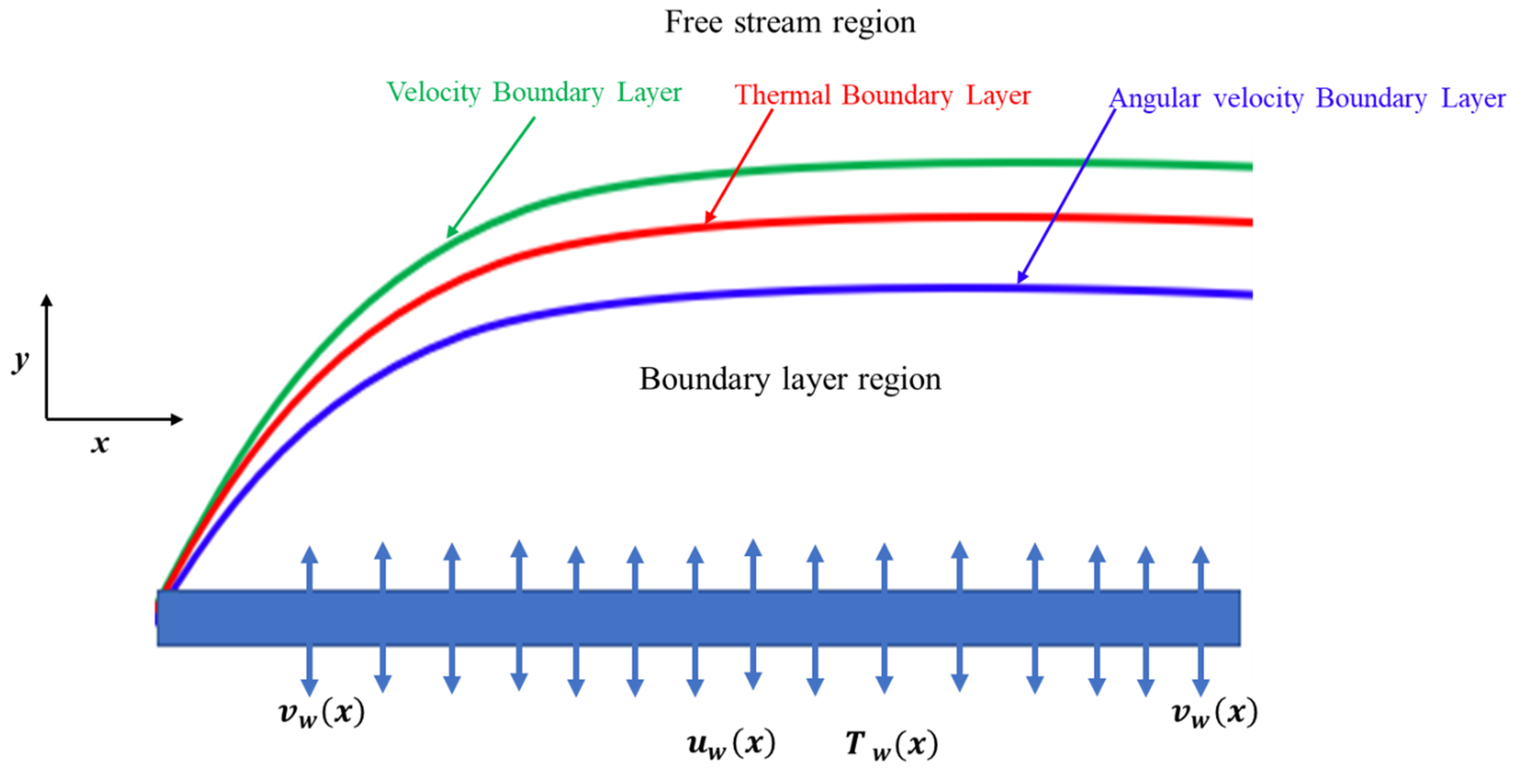
2. Mathematical Formulation

An incompressible laminar boundary layer two-dimensional flow of the micropolar fluid over the exponentially shrinking sheet has been considered. The corresponding velocities of x and y-axes are u and v. The shrinking velocity is assumed to be u w ( x ) = U w e 2 x . The temperature of the sheet is taken to be T   w ( x ) = T + T 0 e x 2 , as shown in Figure 1. The N = N(x,y) is supposed as the angular velocity. The respective boundary layer movement equation, along with micro rotations and the heat transfer equations can be expressed as vectors in accordance with the abovementioned assumptions.
· V = 0
ρ d V d t = P + ( μ + κ ) 2 V + κ ( × N )
ρ j d N d t = γ 2 N κ ( 2 N × V )
ρ c p d T d t = k 2 T
in which velocity vector is V [ u ( x , y ) , v ( x , y ) , 0 ] , the micro-rotation vector is N , ρ stands for fluid density, µ for viscosity coefficient, κ for vertex viscosity, j is the density of micro-rotation, and γ stands for micropolar constant. We get following boundary layer equations according to the scale analysis.
u x + v y = 0
u   u x + v   u y = ( ϑ + κ ρ ) 2 u y 2 + κ ρ N y
u N x + v N y = γ ρ j 2 N y 2 κ ρ j ( 2 N + u y )
u   T x + v   T y = α   2 T y 2
Subject to these boundary conditions
v = v w ( x ) ;       u = u w ( x ) ;     N = m u y ;     T = T   w ( x ) ;       a t         y = 0 u 0 ;   N 0 ;     T T               a s     y
Now, we look for similarity transformation variables in order to transform Equations (6)–(8) with boundary conditions (9)
u = U w e x l f ( η ) ; v = ϑ U w 2 l e x 2 l ( f ( η ) + η f ( η ) ) ; N = U w e 3 x 2 l U w 2 ϑ l h ( η ) ; θ ( η ) = ( T T ) ( T w T ) ;   η = y U w 2 ϑ l   e x 2 l
By applying Equation (10) in Equations (6)–(9), we have the following system of similarity transformed ordinary differential equations
( 1 + K ) f + f f 2 f 2 + K h = 0
( 1 + K 2 ) h + f h 3 f h K ( 2 h + f ) = 0
1 P r θ + f θ f θ = 0
Subject to boundary conditions
f ( 0 ) = S ;     f ( 0 ) = 1 ;     h ( 0 ) = n f ( 0 ) ;     θ ( 0 ) = 1 f ( η ) 0 ;   h ( η ) 0 ;   θ ( η ) 0 ;         a s   η
where prime denotes the differentiation with respect to η , the micropolar material parameter is K = κ μ , Prandtl number is P r = ϑ α , and suction is S = v w ϑ U w / 2 l .
The physical quantities of interest include skin friction, the stress of local couples, and the local number of Nusselt, which are described as
C f = [ ( μ + κ ) u y + κ N ] y = 0 ρ u w 2 ; M x = γ [ N y ] y = 0 ρ x u w 2 ;   N u = x [ T y ] y = 0 ( T w T )
By applying similarity transformation variables (10) in Equation (15), we have
C f ( R e x ) 1 2 2 l / x = ( 1 + ( 1 m ) K ) f ( 0 ) , M x R e x = ( 1 + K 2 ) h ( 0 ) , N u ( R e x ) 1 2 2 l / x = θ ( 0 )
where R e x = x u w / ϑ is the local Reynolds number.

3. Stability Analysis

According to Nasir et al., [28] and Rana et al., [25], we need to introduce the unsteady form of Equations (6)–(8) in order to perform stability test,
u t + u   u x + v   u y = ( ϑ + κ ρ ) 2 u y 2 + κ ρ N y
N t + u N x + v N y = γ ρ j 2 N y 2 κ ρ j ( 2 N + u y )
    T t + u   T x + v   T y = k * ρ c p 2 T y 2
where time is denoted by t. The similarity transformations are written according to Roşca and Pop [30], as,
ψ = 2 ϑ L a e x 2 L f ( η , τ ) ;     N = a e 3 x 2 L a 2 ϑ L h ( η , τ ) ; θ ( η , τ ) = ( T T ) ( T w T ) ; η = y a 2 ϑ L   e x 2 L   ;   τ = a 2 L e x L . t
By applying these similarity transformations, we reduced our Equations (17)–(19) into the following form
( 1 + K ) 3 f η 3 + f 2 f η 2 2 ( f η ) 2 + K h η 2 f τ η = 2 τ ( f η 2 f η x 2 f η 2 f x )
( 1 + K 2 )   2 h η 2 + f h η 3 h f η 2 K h K 2 f η 2 h τ = 2 τ ( f η h x h η f x )
1 P r 2 θ η 2 + f θ η θ f η θ τ = 2 τ ( f η θ x θ η f x )
with the following boundary conditions
f ( 0 , τ ) = S ;   f ( 0 ,   τ ) η = 1 ;     h ( 0 , τ ) = m 2 f ( 0 ,   τ ) η 2 ;   θ ( 0 , τ ) = 1 f ( η ,   τ ) η 0 ;   h ( η , τ ) 0 ;   θ ( η , τ ) 0                     a s   η
and then we applied perturbed with the disturbance (see Roşca and Pop [30]) in Equations (21)–(24) with the following functions
f ( η , τ ) = f 0 ( η ) + e ε τ F ( η , τ ) h ( η , τ ) = h 0 ( η ) + e ε τ G ( η , τ ) θ ( η , τ ) = θ 0 ( η ) + e ε τ H ( η , τ )
where F ( η , τ ) , G ( η , τ ) , and H ( η , τ )   are small relative to f 0 ( η ) , h 0 ( η ) , and θ 0 ( η ) , respectively. Further, ε is the unknown eigenvalue. By substituting Equation (25) in Equations (21)–(23) by keeping τ = 0 , we have following the linearized eigenvalue problems
( 1 + K ) F 0 + f 0 F 0 + F 0 f 0 4 f 0 F 0 + K G 0 + ε F 0 = 0
( 1 + K 2 ) G 0 + f 0 G 0 + F 0 h 0 3 h 0 F 0 3 h 0 F 0 2 K G 0 K F 0 + ε G 0 = 0
1 P r H 0 + f 0 H 0 + F 0 θ 0 f 0 H 0 F 0 θ 0 + ε H 0 = 0
With the boundary conditions
F 0 ( 0 ) = 0 ,             F 0 ( 0 ) = 0 ,         G 0 ( 0 ) = n F 0 ( 0 ) ,           H 0 ( 0 ) = 0 F 0 ( η ) 0 ,       G 0 ( η ) 0 ,               H 0 ( η ) 0 ,             a s     η    
We have to solve above linearized Equations (10)–(13) with new relax boundary conditions in order to find the values of smallest eigenvalue. In this particular problem, we have relaxed H 0 ( η ) 0 as η into H 0 ( 0 ) = 1 , see [31,32,33].

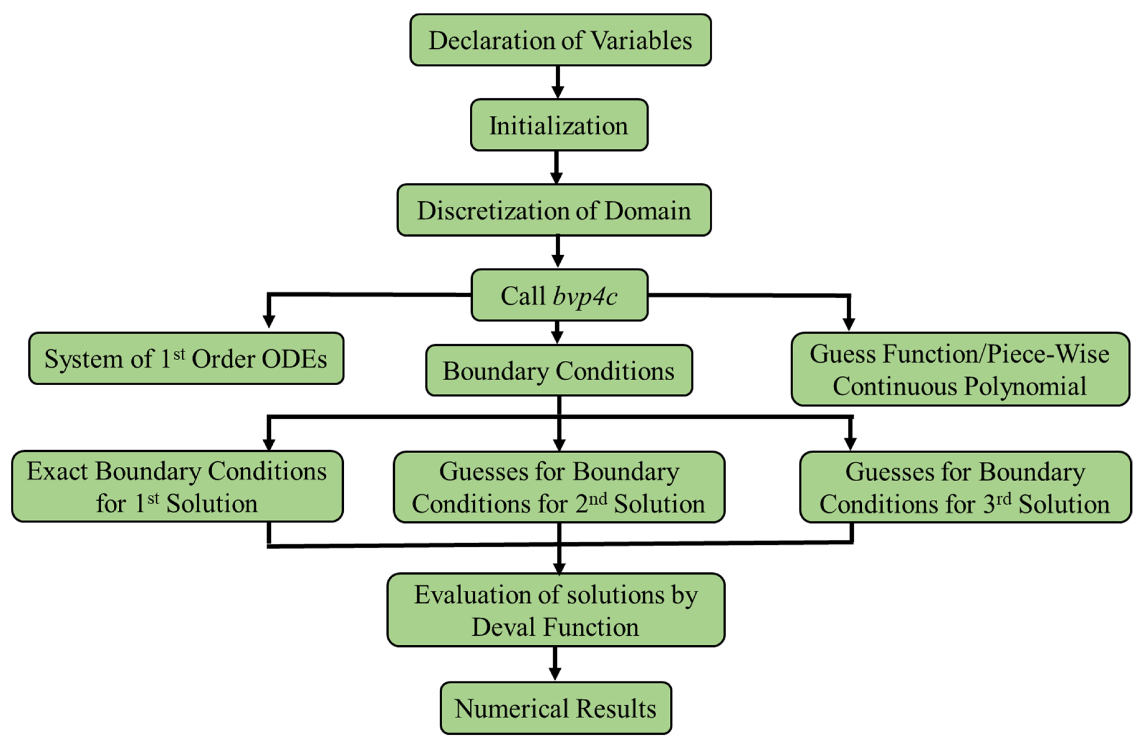
4. Numerical Methods

The governing ODEs are highly non-linear and, therefore, we adopt the numerical approach in order to solve Equations (11)–(14) and Equations (26)–(19). In this study, two methods have been employed, namely shooting method and Three-stage Lobatto III-A formula, which were used in many research articles of same authors previously [refer to 17,20,23,26]. The descriptions regarding these methods are explained below.

4.1. Shooting Method

The shooting technique along with the Runge Kutta method of the fourth order is employed in order to obtain the numerical solutions of Equations (11)–(13) subject to the boundary conditions. Shooting method helps to reduce the third order ODEs (11)–(13) into the first-order ODEs, such that
p = f , q = p ,   r = h ;   q = 1 1 + K { 2 p 2 f q K r }
r = h ;   r = 2 2 + K { 3 p h f r + K ( 2 h + q ) }
s = θ ;   s = P r { p θ f s }
with conditions
f ( 0 ) = S ;   p ( 0 ) = 1 ;   q ( 0 ) = α 1 ;   h ( 0 ) = n α 1 ; r ( 0 ) = α 2 ;   θ ( 0 ) = 1 ; s ( 0 ) = α 3
where α 1 , α 2 , and α 3 are called as unknown initial conditions. These three missing values α 1 , α 2 , and α 3 have to be obtained by using different shoots; this process of shoots will be continue until the profiles of the f ( η ) 0 ;   h ( η ) 0 ; and   θ ( η ) 0   are satisfied the boundary condition   η . Maple (18) software has been used to convert the system of the third order ODEs into the system of the first order ODEs, for this process shootlib function is built-in Maple. Using RK method solves the system of the first order ODEs. Further, a detailed discussion about the shooting method with Maple software can be seen in the paper of Meade et al. [34].

4.2. Three-Stage Lobatto III-A Formula

Three-stage Lobatto III-A formula is built in BVP4C function with aid of C 1 piece-wise cubic polynomial in the finite difference code. According to Lund et al., [35] and Raza et al., [36], “this collocation polynomial and formula offers a C 1 continuous solution in which mesh error control and selection are created on the residual of the continuous solution. The tolerance of relative error is fixed 10 5 for the current problem. The suitable mesh determination is created and returned in the field sol.x. The bvp4c returns solution, called as sol.y., as a construction. In any case, values of the solution are gotten from the array named sol.y relating to the field sol.x”. In addition, Figure 2 explains the algorithm of the method for stability analysis of the solutions.

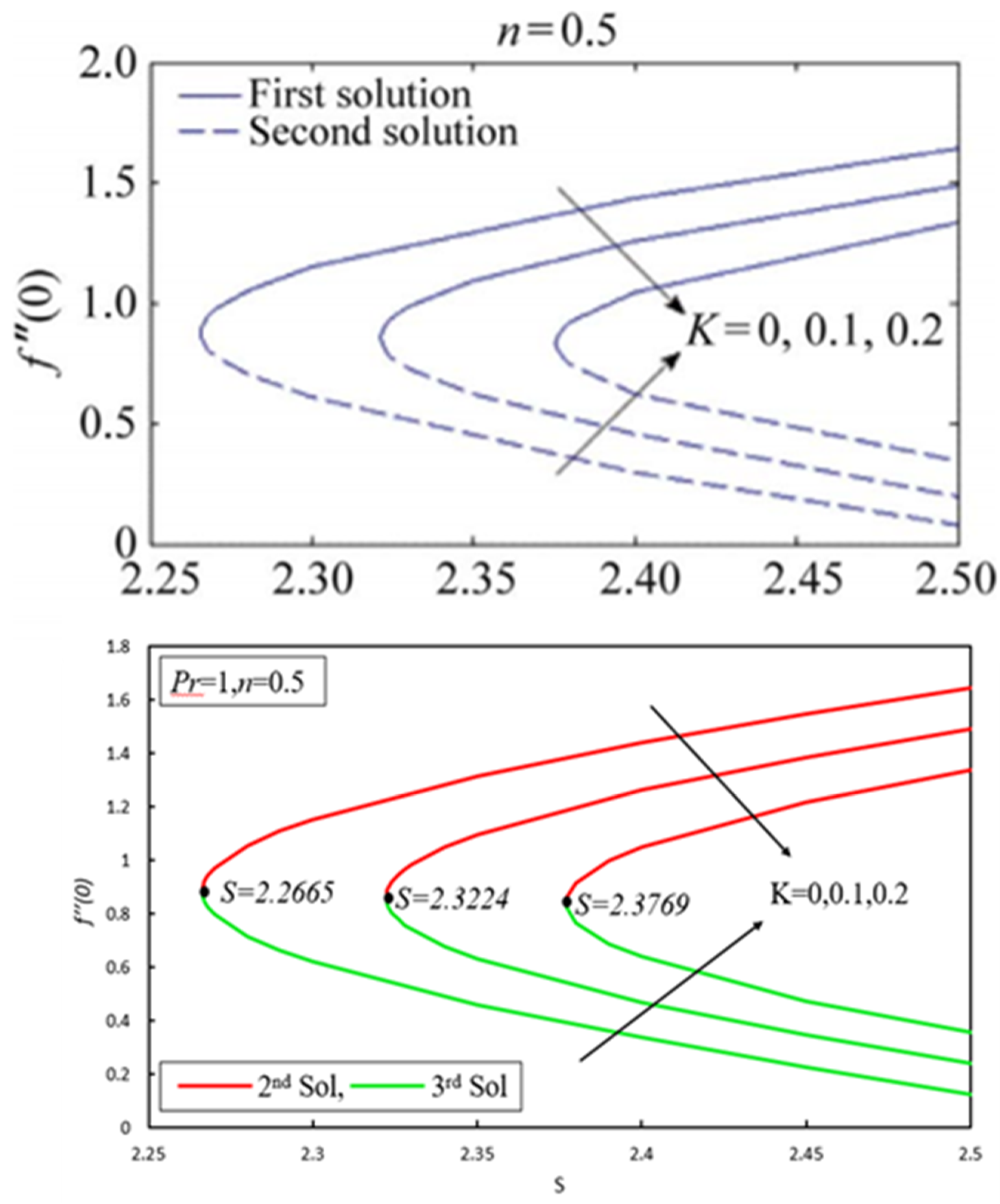
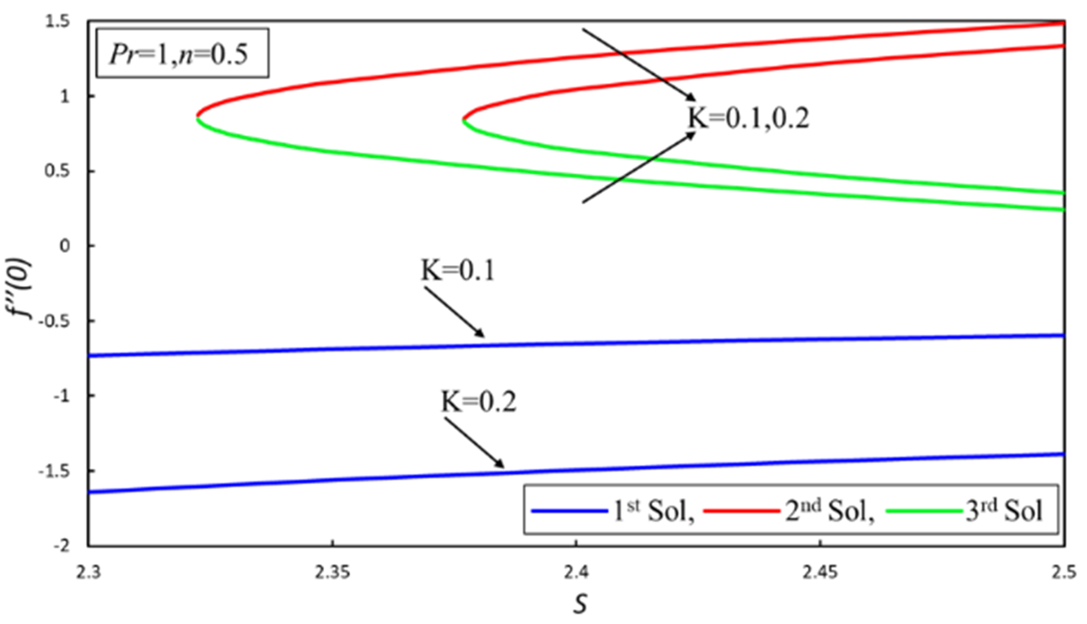
5. Result and Discussion

Aurangzaib et al., [29] solved these Equations (11)–(14) and found dual solutions, which was the main contribution of authors. Aurangzaib et al., [29] have given some strong statements during the investigation of critical points. Before going to detail, we check the accuracy of our method (shooting method) by comparing our results with previously published literature in Table 1 and found excellent agreement with them. Moreover, we also qualitatively compared our results with Aurangzaib et al., [29] in Figure 3 and found in the good agreement. This gives trust in our numerical calculation and urges us to additionally contemplate this problem. Aurangzaib et al., [29] found dual solutions and stated in the result and discussion section that “the present study shows that for K = 0.1, i.e., for micropolar fluid, the similarity solutions exist when S 2.3231 and no similarity solution exists for S < 2.3231 ”. Firstly, we would like to clarify that there exist triple solutions not dual solutions; secondly, there is a range of multiple solutions and single solution. From Figure 4, a conclusion can be made that there exists multiple similarity solutions when S 2.3224 and only a single similarity solution exists for   S < 2.3224 when K = 0.1. However, the range of multiple similarity solution is 2.3769 S and there also exists only a single solution when S < 2.3769 when K = 0.2 (see Figure 4). Furthermore, skin friction increases as suction is increased in the third solution. It is worth mentioning here that there is no range of no solution. This is one of the big reasons that insist us to reconsider and re-examine the whole problem by reproducing all of the results because there are triple solutions in order to provide true knowledge to the readers and researchers.
Figure 5 illustrates the effect of micropolar parameter on the h ( 0 ) . The effect of local couple stress enhanced as the suction increases in the first and third solutions because increasing suction creates additional resistance in the flowing fluid inside the boundary layer. However, increments in the material parameter produce more coupling of stress. Figure 6 shows the nature of the heat transfer rate for various values of the suction. It has been examined that the heat transfer rate increases in the first and second solutions for the higher values of the suction parameter, while the third solution shows opposite compliance.
Finally, we plot Figure 7, Figure 8, Figure 9 and Figure 10 to show the existence of triple solutions of velocity, microrotation, and temperature profiles for different values of material parameter K. In Figure 7, the dual nature of behavior has been noticed in the first solution. Velocity profile increases in the second solution when K is increased; the physical material parameter reduces the effect of drag force due to that thickness of the momentum boundary layer enhanced. On the other hand, the opposite trend has been observed in the third solution. Dual behavior can be noticed microrotation profile in Figure 8 for all solutions. The thickness of thermal boundary layer increases in the first and second solutions as material parameter K is increased, as in Figure 9, since the non-Newtonian parameter produces more viscosity, decreases the velocity of profiles, and forces fluid flow to stay on the hotter surface, as a result temperature of fluid increases and the boundary layer becomes thicker. However, the opposite behavior is noticed for the third solution. The Prandtl effect on the temperature distribution is depicted in Figure 10. It is observed that the temperature of fluid diminishes for the higher values of the Prandtl number for all solutions. Physically, it can be explained, as the Prandtl number ( P r = μ c p k ) has an inverse relationship with the thermal conductivity and, consequently, diminishes the thickness of the thermal boundary layer.
Table 2 shows the smallest eigenvalues ε for the selected values of S and K. The positive smallest eigenvalue makes the initial disturbance decay and, in this way, the flow becomes stable. Conversely, the negative smallest eigenvalue outcomes in an initial growth of disturbance, in this manner, the flow is unstable. It is seen from Table 2 that ε is negative for the second and the third solutions, while positive for the first solution. Thus, the second and the third solution are not stable, and the first solution is stable. From this discussion, it can be concluded that the first solution of Aurangzaib et al., [29] is not stable and not physically realizable; therefore, in this stage, it could be said that the first solution is actually the second or the third solution.

6. Conclusions

The micropolar fluid over the shrinking surface has been considered. The system of governing equations has been transformed into the system of ODEs by using appropriate exponential similarity transformation. The system of ODEs is reduced to IVPs by employing the shooting method before solving IVPs by the Runge Kutta method. The pointwise conclusions of this study are given below:
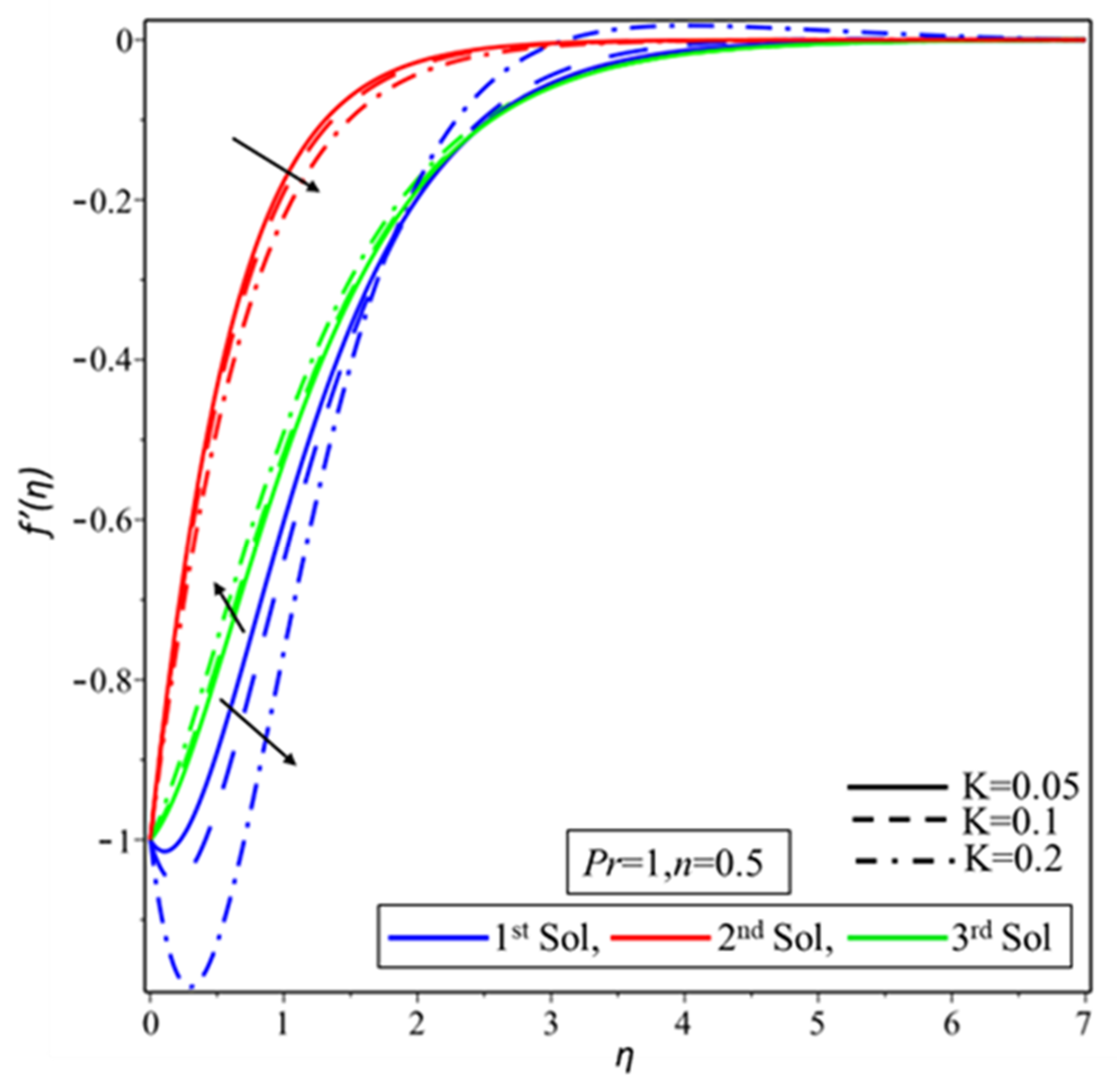
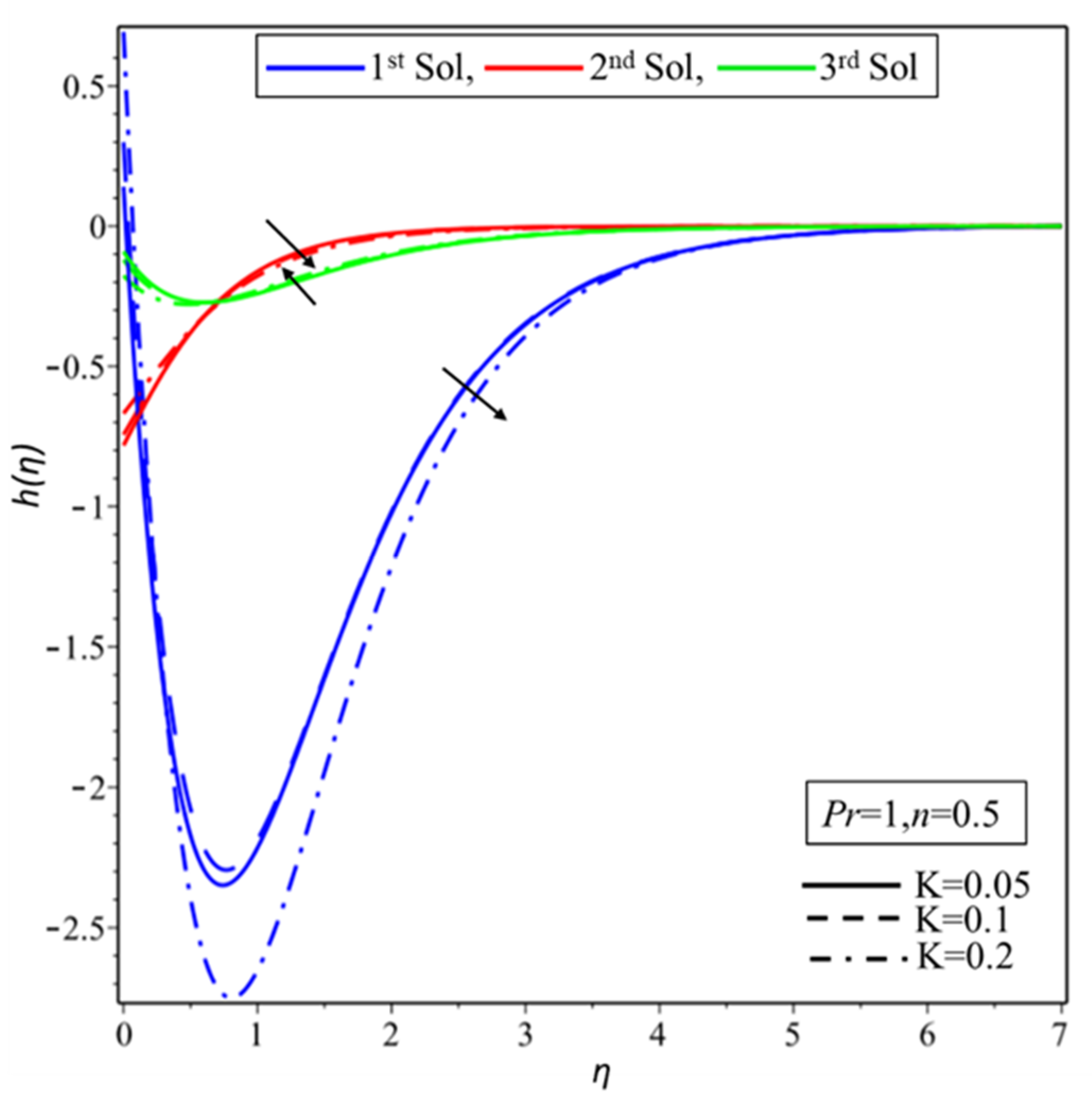
  • Triple solutions appear.
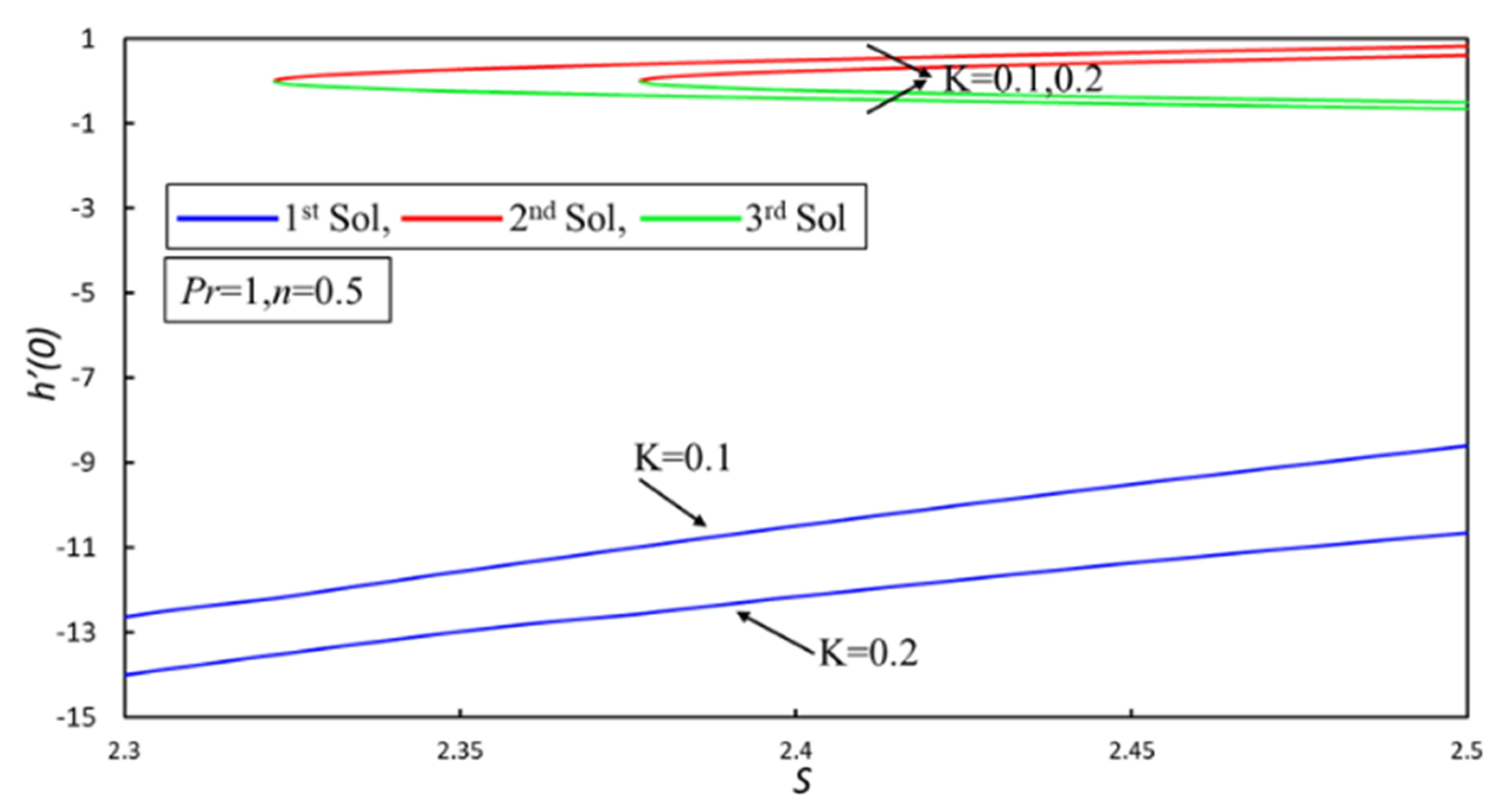
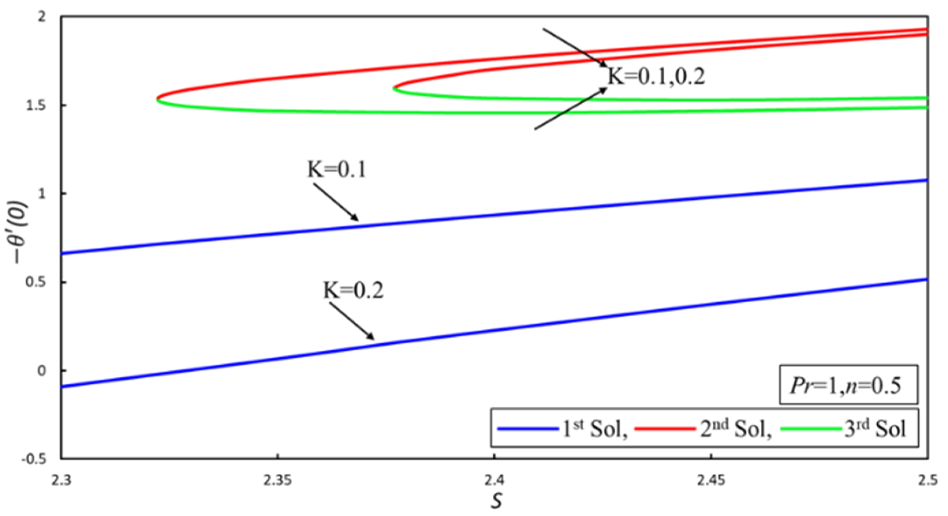
  • There are ranges of multiple solutions and no solutions that depend upon the suction parameter.
  • According to stability analysis, the first solution is stable, which can be experimentally seen.
  • The results of Aurangzaib et al., [29] are unstable.
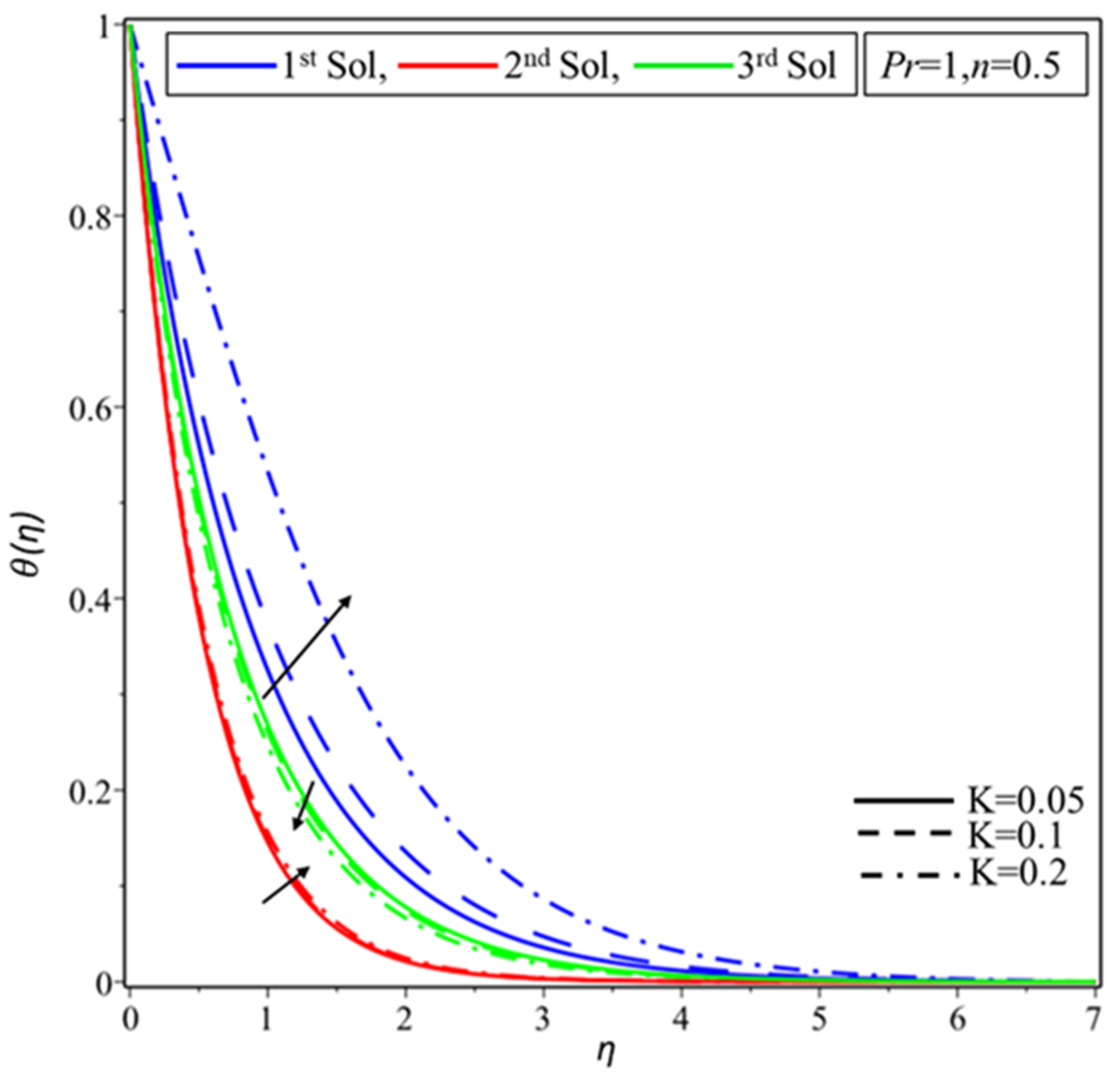
  • The thickness of thermal boundary layer increases in the first and the second solutions as material parameter K is increased.
  • Increments in the material parameter produce more couple stress.

Author Contributions

Conceptualization, L.A.L. and Z.O.; Funding acquisition, D.B.; Investigation, I.K.; Methodology, L.A.L., and I.K.; Project administration, I.K.; Software, L.A.L., I.K., Z.O., D.B., and K.S.N.; Supervision, I.K.; Review and Revision: D.B. and K.S.N.; Formal Analysis: D.B. and K.S.N. All authors have read and agreed to the published version of the manuscript.

Funding

This research is also supported by the Universiti Utara Malaysia.

Acknowledgments

This project was supported by the Deanship of Scientific Research at Prince Sattam Bin Abdulaziz University under the research project No. 2020/01/16436.The first author is thankful to his all teachers, especially Prof. Mazhar Ali Lund (U. B Govt. Degree college Dadu) who taught him free of cost in 2007–2009.

Conflicts of Interest

The authors declare no conflict of interest.

References

  1. Eringen, A. Simple microfluids. Int. J. Eng. Sci. 1964, 2, 205–217. [Google Scholar] [CrossRef]
  2. Eringen, A.C. Theory of micropolar fluids. J. Math. Mech. 1966, 16, 1–18. [Google Scholar] [CrossRef]
  3. Lukaszewicz, G. Micropolar Fluids: Theory and Applications; Springer Science & Business Media: Berlin/Heidelberg, Germany, 1999. [Google Scholar]
  4. Eringen, A.C. Microcontinuum Field Theories: II. Fluent Media (Vol. 2); Springer Science & Business Media: Berlin/Heidelberg, Germany, 2001. [Google Scholar]
  5. Lok, Y.Y.; Ishak, A.; Pop, I. Oblique stagnation slip flow of a micropolar fluid towards a stretching/shrinking surface: A stability analysis. Chin. J. Phys. 2018, 56, 3062–3072. [Google Scholar] [CrossRef]
  6. Sheremet, M.; Pop, I.; Ishak, A. Time-dependent natural convection of micropolar fluid in a wavy triangular cavity. Int. J. Heat Mass Transf. 2017, 105, 610–622. [Google Scholar] [CrossRef]
  7. Bhattacharyya, K.; Mukhopadhyay, S.; Layek, G.; Pop, I. Effects of thermal radiation on micropolar fluid flow and heat transfer over a porous shrinking sheet. Int. J. Heat Mass Transf. 2012, 55, 2945–2952. [Google Scholar] [CrossRef]
  8. Ishak, A.; Nazar, R.; Pop, I. Dual solutions in mixed convection boundary layer flow of micropolar fluids. Commun. Nonlinear Sci. Numer. Simul. 2009, 14, 1324–1333. [Google Scholar] [CrossRef]
  9. Ramzan, M.; Farooq, M.; Hayat, T.; Chung, J.D. Radiative and Joule heating effects in the MHD flow of a micropolar fluid with partial slip and convective boundary condition. J. Mol. Liq. 2016, 221, 394–400. [Google Scholar] [CrossRef]
  10. Turkyilmazoglu, M. Mixed convection flow of magnetohydrodynamic micropolar fluid due to a porous heated/cooled deformable plate: Exact solutions. Int. J. Heat Mass Transf. 2017, 106, 127–134. [Google Scholar] [CrossRef]
  11. Shah, Z.; Islam, S.; Ayaz, H.; Khan, S. Radiative Heat and Mass Transfer Analysis of Micropolar Nanofluid Flow of Casson Fluid Between Two Rotating Parallel Plates With Effects of Hall Current. J. Heat Transf. 2018, 141, 022401. [Google Scholar] [CrossRef]
  12. Lund, L.A.; Ching, D.L.C.; Omar, Z.; Khan, I.; Nisar, K.S. Triple Local Similarity Solutions of Darcy-Forchheimer Magnetohydrodynamic (MHD) Flow of Micropolar Nanofluid Over an Exponential Shrinking Surface: Stability Analysis. Coatings 2019, 9, 527. [Google Scholar] [CrossRef] [Green Version]
  13. Lund, L.A.; Omar, Z.; Khan, U.; Khan, I.; Baleanu, D.; Nisar, K.S. Stability Analysis and Dual Solutions of Micropolar Nanofluid over the Inclined Stretching/Shrinking Surface with Convective Boundary Condition. Symmetry 2020, 12, 74. [Google Scholar] [CrossRef] [Green Version]
  14. Dero, S.; Rohni, A.M.; Saaban, A. MHD Micropolar Nanofluid Flow over an Exponentially Stretching/Shrinking Surface: Triple Solutions. J. Adv. Res. Fluid Mech. Therm. Sci. 2019, 56, 165–174. [Google Scholar]
  15. Lund, L.A.; Omar, Z.; Khan, I. Mathematical analysis of magnetohydrodynamic (MHD) flow of micropolar nanofluid under buoyancy effects past a vertical shrinking surface: Dual solutions. Heliyon 2019, 5, e02432. [Google Scholar] [CrossRef] [PubMed] [Green Version]
  16. Lund, L.A.; Omar, Z.; Dero, S.; Khan, I. Linear stability analysis of MHD flow of micropolar fluid with thermal radiation and convective boundary condition: Exact solution. Heat Transf.-Asian Res. 2019, 49, 461–476. [Google Scholar] [CrossRef]
  17. Raza, J.; Rohni, A.M.; Omar, Z. Rheology of micropolar fluid in a channel with changing walls: Investigation of multiple solutions. J. Mol. Liq. 2016, 223, 890–902. [Google Scholar] [CrossRef]
  18. Rohni, A.M. Multiple Similarity Solutions of Steady and Unsteady Convection Boundary Layer Flows in Viscous Fluids and Nanofluids. Ph.D. Thesis, Universiti Sains Malaysia, Penang, Malaysia, 2013. [Google Scholar]
  19. Mishra, S.; Debroy, T. A computational procedure for finding multiple solutions of convective heat transfer equations. J. Phys. D Appl. Phys. 2005, 38, 2977–2985. [Google Scholar] [CrossRef]
  20. Lund, L.A.; Omar, Z.; Khan, I.; Dero, S. Multiple solutions of Cu-C6H9NaO7 and Ag-C6H9NaO7 nanofluids flow over nonlinear shrinking surface. J. Cent. South Univ. 2019, 26, 1283–1293. [Google Scholar] [CrossRef]
  21. Khashi’Ie, N.S.; Arifin, N.M.; Nazar, R.; Hafidzuddin, E.H.; Wahi, N.; Pop, I. Mixed Convective Flow and Heat Transfer of a Dual Stratified Micropolar Fluid Induced by a Permeable Stretching/Shrinking Sheet. Entropy 2019, 21, 1162. [Google Scholar] [CrossRef] [Green Version]
  22. Raza, J.; Rohni, A.M.; Omar, Z. A Note on Some Solutions of Copper-Water (Cu-Water) Nanofluids in a Channel with Slowly Expanding or Contracting Walls with Heat Transfer. Math. Comput. Appl. 2016, 21, 24. [Google Scholar] [CrossRef] [Green Version]
  23. Lund, L.A.; Omar, Z.; Khan, I.; Raza, J.; Bakouri, M.; Tlili, I. Stability Analysis of Darcy-Forchheimer Flow of Casson Type Nanofluid Over an Exponential Sheet: Investigation of Critical Points. Symmetry 2019, 11, 412. [Google Scholar] [CrossRef] [Green Version]
  24. Dero, S.; Uddin, M.J.; Rohni, A.M. Stefan Blowing and Slip Effects on Unsteady Nanofluid Transport Past a Shrinking Sheet: Multiple Solutions. Heat Transfer-Asian Res. 2019, 48, 2047–2066. [Google Scholar] [CrossRef]
  25. Rana, P.; Shukla, N.; Gupta, Y.; Pop, I. Analytical prediction of multiple solutions for MHD Jeffery–Hamel flow and heat transfer utilizing KKL nanofluid model. Phys. Lett. A 2019, 383, 176–185. [Google Scholar] [CrossRef]
  26. Lund, L.A.; Omar, Z.; Khan, I. Analysis of dual solution for MHD flow of Williamson fluid with slippage. Heliyon 2019, 5, e01345. [Google Scholar] [CrossRef] [PubMed] [Green Version]
  27. Waini, I.; Ishak, A.; Pop, I. Unsteady flow and heat transfer past a stretching/shrinking sheet in a hybrid nanofluid. Int. J. Heat Mass Transf. 2019, 136, 288–297. [Google Scholar] [CrossRef]
  28. Nasir, N.A.A.M.; Ishak, A.; Pop, I. Stagnation point flow and heat transfer past a permeable stretching/shrinking Riga plate with velocity slip and radiation effects. J. Zhejiang Univ. A 2019, 20, 290–299. [Google Scholar] [CrossRef]
  29. Aurangzaib; Uddin, S.; Bhattacharyya, K.; Khan, I. Micropolar fluid flow and heat transfer over an exponentially permeable shrinking sheet. Propuls. Power Res. 2016, 5, 310–317. [Google Scholar] [CrossRef]
  30. Roşca, A.V.; Pop, I. Flow and heat transfer over a vertical permeable stretching/shrinking sheet with a second order slip. Int. J. Heat Mass Transf. 2013, 60, 355–364. [Google Scholar] [CrossRef]
  31. Rahman, M.; Roşca, A.; Pop, I. Boundary layer flow of a nanofluid past a permeable exponentially shrinking/stretching surface with second order slip using Buongiorno’s model. Int. J. Heat Mass Transf. 2014, 77, 1133–1143. [Google Scholar] [CrossRef]
  32. Harris, S.D.; Ingham, D.B.; Pop, I. Mixed Convection Boundary-Layer Flow Near the Stagnation Point on a Vertical Surface in a Porous Medium: Brinkman Model with Slip. Transp. Porous Media 2008, 77, 267–285. [Google Scholar] [CrossRef]
  33. Ishak, A. MHD boundary layer flow due to an exponentially stretching sheet with radiation effect. Sains Malays. 2011, 40, 391–395. [Google Scholar]
  34. Meade, D.B.; Haran, B.S.; White, R.E. The shooting technique for the solution of two-point boundary value problems. Maple Tech. Newsl. 1996, 3, 1–8. [Google Scholar]
  35. Lund, L.A.; Omar, Z.; Khan, I. Quadruple solutions of mixed convection flow of magnetohydrodynamic nanofluid over exponentially vertical shrinking and stretching surfaces: Stability analysis. Comput. Methods Programs Biomed. 2019, 182, 105044. [Google Scholar] [CrossRef] [PubMed]
  36. Raza, J.; Mebarek-Oudina, F.; Chamkha, A. Magnetohydrodynamic flow of molybdenum disulfide nanofluid in a channel with shape effects. Multidiscip. Model. Mater. Struct. 2019, 15, 737–757. [Google Scholar] [CrossRef]
  37. Pramanik, S. Casson fluid flow and heat transfer past an exponentially porous stretching surface in presence of thermal radiation. Ain Shams Eng. J. 2014, 5, 205–212. [Google Scholar] [CrossRef] [Green Version]
  38. Raju, C.S.K.; Sandeep, N.; Sugunamma, V.; Babu, M.J.; Reddy, J.R. Heat and mass transfer in magnetohydrodynamic Casson fluid over an exponentially permeable stretching surface. Eng. Sci. Technol. Int. J. 2016, 19, 45–52. [Google Scholar] [CrossRef] [Green Version]
Figure 1. Flow of problem and coordinate system.
Crystals 10 00283 g001
Figure 2. Description of three-stage Lobatto III-A formula.
Crystals 10 00283 g002
Figure 3. Comparison between upper graph: existing results obtained by Aurangzaib et al., [29] and lower graph: present results.
Crystals 10 00283 g003
Figure 4. Variation of f ( 0 ) for different fixed values of K with suction parameter S.
Crystals 10 00283 g004
Figure 5. Variation of h ( 0 ) for different fixed values of K with suction parameter S.
Crystals 10 00283 g005
Figure 6. Variation of θ ( 0 ) for different fixed values of K with suction parameter S.
Crystals 10 00283 g006
Figure 7. Effect of K on f ( η ) when S = 2.5.
Crystals 10 00283 g007
Figure 8. Effect of K on h ( η ) when S = 2.5.
Crystals 10 00283 g008
Figure 9. Effect of K on θ ( η ) when S = 2.5.
Crystals 10 00283 g009
Figure 10. Effect of Pr on θ ( η ) .
Crystals 10 00283 g010
Table 1. The comparison of values of heat transfer rate for different values of Pr.
PrMIshak [33]Pramanik [37]Raju et al. [38]Present Results
100.95480.95470.9547340.954955
201.47151.47141.4714261.471421
301.86911.86911.8691341.869044
1003.66033.66033.6603123.660354
Table 2. Smallest eigen values ε at several values of S and K when Pr = 1.
KS ε
1st solution2nd solution3rd solution
0.12.32241.2806100
-2.41.0662−0.06382−0.13406
0.22.37691.3620100
-2.41.1364−0.10482−0.17482

