A Novel Approach to Modelling Nanoindentation Instabilities

Materials Research Centre, Indian Institute of Science, Bangalore 560012, India
*
Author to whom correspondence should be addressed.
Crystals 2018, 8(5), 200; https://0-doi-org.brum.beds.ac.uk/10.3390/cryst8050200
Submission received: 17 January 2018
/
Revised: 25 April 2018
/
Accepted: 27 April 2018
/
Published: 3 May 2018
(This article belongs to the Special Issue Crystal Indentation Hardness)
Abstract
:We review the recently developed models for load fluctuations in the displacement controlled mode and displacement jumps in the load controlled mode of indentation. To do this, we devise a method for calculating plastic contribution to load drops and displacement jumps by setting-up a system of coupled nonlinear time evolution equations for the mobile and forest dislocation densities by including relevant dislocation mechanisms. These equations are then coupled to the equation defining constant displacement rate or load rate. The model for the displacement controlled mode using a spherical indenter predicts all the generic features of nanoindentation such as the elastic branch followed by several force drops of decreasing magnitudes and residual indentation depth after unloading. The stress corresponding to the elastic force maximum is close to the yield stress of an ideal solid. The predicted numbers for all the quantities match experiments on single crystals of Au using a spherical indenter. We extend the approach to model the load controlled nanoindentation experiments that employ a Berkovich indenter. We first identify the dislocation mechanisms contributing to different regions of the curve as a first step for obtaining a good fit to a given experimental curve. This is done by studying the influence of the parameters associated with various dislocation mechanisms on the model curves. The study also demonstrates that the model predicts all the generic features of nanoindentation such as the existence of an initial elastic branch followed by several displacement jumps of decreasing magnitudes and residual plasticity after unloading for a range of model parameter values. Furthermore, an optimized set of parameter values can be easily determined that give a good fit to the experimental load–displacement curves for Al single crystals of and orientations. Our model also predicts the indentation size effect in a region where the displacement jumps disappear. The good agreement of the results of the models with experiments supports our view that the present approach can be used as an alternate method to simulations. The approach also provides insights into several open questions.
1. Introduction
The fact that mechanical properties of small volume systems are different from the bulk has been evident in a number of early studies. For instance, the high strength of whiskers is due to the absence of dislocations [1,2]. Similarly, the grain boundary strengthening mechanism is due to the fact that dislocation motion is limited by the grain size, and the dynamic friction (wear) is controlled by the plastic deformation of micrometer or sub-micrometer asperities [3]. There has been a spurt of activity in size dependent studies on plastic deformation of small volume systems in the last three decades due to technological importance as well as the scientific challenges it offers. For instance, intermittent flow is observed when the diameter of micrometer rods are below a certain value while it is smooth when it is large implying the instability manifests when the aspect ratio is reduced [4,5,6]. Similar intermittent plastic flow in the form of load fluctuations or displacement jumps is reported when the indentation depth is less than 100 nm both in thin and bulk samples [7,8,9,10,11,12]. Thus, nanoindentation experiments fall into the class of experiments where plastic instability manifests due to small deformed volume [7,8,9,10,11,12].
Traditionally, two modes of nanoindentation experiments are employed, namely, load/force controlled (LC) mode or displacement controlled (DC) mode [7,9,11,13,14,15]. In both modes, experiments measure the force response of the sample (to the applied force) as a function of indentation depth. While several load drops of decreasing magnitudes are seen in the DC mode experiments [7,9,11,13,14,15], several displacement jumps of decreasing magnitudes are seen beyond the elastic limit in the LC mode experiments [10,12,14,16,17]. The maximum load on the elastic branch is close to the theoretical yield stress. In both modes, residual plasticity is seen after unloading the indenter. While the presence of surface defects, oxide coatings, precipitates, etc. complicate the interpretation of the results, careful and controlled experiments on well-prepared single crystals have demonstrated that the above generic features are reproducible [11,14,15,18]. Since the deformed volume prior to the onset of intermittent plastic flow is a few nm, the standard explanation for the high yield strength is the low probability of finding dislocations in such small deformed volumes. The sequence of load drops in the DC mode and displacement jumps in the LC mode beyond the elastic branch have been considered as signatures of instabilities triggered by bursts of plasticity.
Three distinct types of studies have provided much insight into the nanoindentation process, namely, bubble raft indentation[10], colloidal crystals, which are soft matter equivalent of the crystalline phase [19], and in situ transmission electron microscope studies. The latter, in particular, has been useful in visualizing the dislocation nucleation mechanism in real materials [20]. Finally, considerable theoretical understanding has come from various types of simulation studies such as molecular dynamics (MD) simulations [21,22,23,24,25,26], dislocation dynamics simulations and multiscale modeling simulations (using MD together with dislocation dynamics simulations) [26]. While there are a number of MD simulations for the DC mode, there are no simulations of any kind that predict displacement jumps reported in the LC mode experiments.
However, a serious limitation of these simulations is the limited size of the simulated volumes and short time scales used. More importantly, the indentation rates are often several orders of magnitude higher than those in experiments, raising questions of relevance of these simulations to real materials [23,27]. Furthermore, simulation approaches cannot employ experimental parameters such as the indentation rates or the geometrical parameters defining the indenter, thickness of the sample, etc. As a result, the predicted values of load, indentation depth, etc. differ considerably from those reported by experiments.
The above limitations of simulation methods prompted us to develop an alternate framework that has the ability to adopt laboratory time and length scales to predict numbers that agree with experiments. The purpose of this paper is to review the recently introduced dynamical approach and the models that predict the results for the DC and LC mode nanoindentation experiments [28,29]. The approach is based on our previous experience in modeling a significantly more complex spatio-temporal instability, namely, the Portevin–Le Chatelier (PLC) effect seen in bulk samples of dilute alloys under constant strain rate conditions [30,31,32,33,34]. The approach is applicable to ideal single crystals without any kind of defects.
Our approach to nanoindentation is based on two observations. First, the sequence of load drops (in the DC mode) and the sequence of displacement jumps (in the LC mode) seen beyond the elastic branch are triggered by collective dislocation activity. Second, the intermittent deformation is a signature of an instability. The most suitable mathematical platform for describing instabilities and collective behavior of constituent entities is nonlinear dynamics. Furthermore, since the basic defects contributing to plastic flow are dislocations, a proper description of collective dislocation behavior demands that we include all the relevant dislocation mechanisms contributing to the bursts of plasticity. On the basis of these observations, we recently developed a novel approach [28,29] by combining the power of nonlinear dynamics with a method for calculating the plastic contribution to the indentation depth. The latter is calculated by developing time evolution equations for the mobile and forest dislocation densities based on the knowledge of the dislocation mechanisms contributing to plastic flow [28,29]. In addition, the approach allows us to employ experimental indentation rates, the geometrical parameters defining the indenter, thickness of the film, etc. The efficacy of the approach is illustrated by developing a model for the DC mode nanoindentation experiments (carried out using a spherical indenter) [28]. The model predicts all the generic features of the DC mode with numbers matching experimental results on single crystals of gold [11,15]. We have also developed a model for predicting the displacement jumps in the LC mode indentation even though the exercise is even more challenging due to the conceptual difficulty in enforcing a constant load rate during displacement jumps. Indeed, this difficulty appears to be the reason for a complete absence of any kind of simulations to explain the displacement jumps in the LC mode. Since we plan to get a good fit to the experimental plots [12], we first study the influence of the parameters associated with dislocation mechanisms on the model curves with a view to identify the dislocation mechanisms that control different regions of the curve. The study further demonstrates that the model predicts all the generic features of nanoindentation such as the existence of an initial elastic branch followed by several displacement jumps of decreasing magnitudes and residual plasticity after unloading for a range of values of model parameters associated with the dislocation mechanisms. This also helps us to obtain optimized parameter values that give a good fit to the experimental load–displacement curves for Al single crystals of and orientations [12]. While hardness is not well defined at nanometer scales where displacement jumps dominate, for larger indentation depths where intermittency disappears, the hardness decreases with depth. Thus, indentation size effect is also predicted. These results also justify our expectation that the present approach can be used as an alternate method to simulations in modeling nanoindentation instabilities. These studies also provide insights into several open questions related to the collective behavior of dislocations: (a) Which dislocation mechanisms determine the first and subsequent load drops or displacement jumps? (b) Can all load drops and displacement jumps be explained on the basis of a common physical and mathematical mechanism? (c) What physical and mathematical mechanisms contribute to the decreasing magnitudes of the load drops or displacement jumps?
2. Insights from Simulations on Nanoindentation
At the outset, it must be mentioned that, apart from bubble raft simulation [10], only MD simulations predict load drops in DC mode of nanoindentation. There are no MD simulations (or any other for that matter) for the displacement jumps in the LC mode. In general, simulation methods have always served the purpose of understanding dislocation mechanisms underlying the evolution of complex dislocation microstructures in various dislocation mediated plasticity. The purpose of this section is to briefly summarize the results of MD simulations and multiscale modeling method, and discuss their advantages and limitations.
In the context of simulating the DC mode nanoindentation instability, MD simulations have played an important role in providing a good understanding of initial stages of plastic deformation. However, because of the limited volume that can be simulated, subsequent evolution of the plastic zone becomes prohibitive as indentation proceeds. This has motivated researchers to develop a multi-scale modeling method that uses MD results as a starting point for understanding further evolution of dislocation microstructure using discrete dislocation dynamical (DDD) simulations in conjunction with finite element methods (FEM).
The suitability of these simulations depends on the stage of evolution of dislocation microstructure that is being targeted. Here, we note that the load drops manifest at a few tens of nm scale corresponding to the initial stages of dislocation microstructure. Furthermore, the initial indented volume prior to the onset of plasticity is of the order of 10 nm. On the other hand, typical dislocation density in a well grown single crystals is ∼10m. Thus, the probability of finding a dislocation is close to zero. The nucleated dislocation loops act as the trigger for the pop-in events and therefore represent elastic to plastic transition. Then, MD simulations are best suited for this initial stages of deformation. The typical size of the simulated volume is a few million atoms. However, they are clearly not suitable for simulations when describing further development of plastic zone (beyond say 50 nm). A multi-scale method has been developed by Chang et al. [26] that incorporates MD results into discrete dislocation dynamic(DDD) simulations in conjunction with finite element methods to take into account the boundary conditions relevant for the loading condition.
There are a number of MD simulations that capture the evolution of dislocation microstructure to various degrees [21,23,24,25,26]. Features that emerge from these simulations include the nucleation of dislocation loops, their expansion and interaction, detachment from the source, and their propagation [26].
Almost all studies use a spherical indenter, which is modeled using a repulsive potential. Different kinds of potentials have been used (to simulate the desired crystal) in MD simulations. Typical large MD simulations use a million atoms and the radius of the indenter can range from about 0.8 nm to 15 nm [21,23,24,25,26]. Typical rates of indentation are ∼/step with each step typically a few ps duration required to attain minimum energy configuration. Typical indentation depths are about 10 Å and the force is ∼N to a few N.
For illustration, we use the results of Van Vliet et al. [23]. These authors use Ercolessi–Adamssi potential to simulate Aluminum. The load–displacement curve with several load drops is shown in Figure 1a. Due to the inherent advantage of MD simulations, dislocation activity (see Figure 9 of Ref. [23]) can be correlated with the load drops in the load–displacement curve. As can be seen, nucleation occurs at 20 nN, which corresponds to a nucleation stress of ∼ 3.4 GPa. The glide loops expand along planes. In addition to nucleation, other dislocation mechanisms the authors realize are the formation of sessile locks, cross-slip, and propagation after detachment from the source. The maximum depth of indentation is . One can also notice small scale fluctuations in the load–displacement curve, an effect well known in MD simulations, even in the context of MD simulations of equilibrium properties. Such fluctuations tend to smooth out as the system size is increased.
In the following, we briefly summarize the results of the multi-scale modeling approach due to Change et al. [26]. To begin with, we briefly recall their MD results. They use an Embedded-atom method type of interatomic potential typical to several other MD simulations. The authors use a repulsive sphere that is pressed into the sample at a rate of at each step of a few ps duration. The top surface is traction-free and the atoms located on the bottom surface are fixed. Periodic boundary conditions are applied in the direction perpendicular to the indentation axis. Figure 1b shows the load–displacement curve with several pop-in events. The first load drop has been identified with the nucleation of three prismatic interstitial dislocation loops. The nucleation occurs at 1 nm and subsequent evolution of dislocation microstructure with indentation depth consists of expansion of the loops, their multiplication followed by detachment from the surface (see Figure 2a–f of Ref. [26]).
The DDD simulations employed by the authors use an Edge-screw code with an FEM solver. The FEM is used to compute the highly heterogeneous stresses during the indentation process. The information about nucleation of dislocation loops seen in MD simulation are incorporated by a set of rules that specify the shape of loops and position of the loops to be introduced in the simulation cell. The imposed displacement rate determines the number of loops introduced. The load–displacement curve using a spherical indenter of radius nm is shown in Figure 2. The figure shows the total load, load contribution from dislocations and the MD result extrapolated to the maximum depth of 100 nm. The evolution of dislocation microstructure becomes increasingly complex as illustrated in Figure 3a–d. For details, see Chang et al. [26].
As can be seen, a major advantage of the MD simulations is their ability to include a range of dislocation mechanisms starting from the nucleation of dislocations, their multiplication, formation of locks, junctions, propagation of loops, etc. [21,23,24,25,26]. Note that these dislocation mechanisms are all used in our model. The most obvious limitation of MD simulations is the limited volume they can simulate. This also means that the maximum radius of a spherical indenter is also limited. This also means that the predicted depths at which nucleation occurs is typically 6–10 Å significantly smaller than in experiments [11,15]. One other important limitation is the length and time scales that are inherent to the small scale simulations. The relaxation time scale to attain the minimum energy configuration is typically a few ps. This coupled with the fact that the loading rates are a fraction of an Å means that the imposed displacement ∼m/s. This is at least orders higher than that used in experiments by Kiely et al., who use [11,15]. On the other hand, while DDD simulations are useful in tracking further development of dislocation microstructure, these simulations do not model the intermittent region. These limitations prompted us to devise an alternate framework that can use experimental conditions such as the imposed rates, geometrical parameters defining the indenter and other experimental parameters.
3. Background Material
This review specifically targets two most popular quasi-static modes of indentation, namely, the displacement controlled indentation where imposed displacement is increased at a constant rate and load controlled mode where the load is increased at a constant rate. These two modes of indentation are primarily chosen because the equations governing the DC and LC modes take a simple form compared to the dynamic loading mode, not considered here. The simplicity of these equations helps us establish a good correlation between imposed rates and plastic response of the material. In addition, for each of these modes of indentation, we can use different types of indenters. Here, we consider (a) spherical indenter for the DC mode with a view to compare the model results with those of Kiely et al. [11,15]), and (b) Berkovich indenter in the LC mode so as to compare our model results with Gouldstone et al. [12]. Here, we consider a single crystal without surface defects, inclusions, precipitates, etc. (Other complications in nanoindentation such as pile-up and sink-in effects are beyond the scope of our approach.). We begin by collecting relevant background material.
In our approach, the indentation depth z measured from the undeformed surface is a dynamical variable, i.e., a variable that evolves with time. The total indentation depth z is the sum of elastic indentation depth and plastic depth . Then,
The elastic depth is essentially known since it is governed by the indenter specific load–depth expression. However, calculating the plastic displacement has been the obstacle for developing any nanoindentation model. The strength of our approach is that it provides a way of calculating by first calculating the plastic strain rate using the Orowan equation [35]. This also means that we use strain as a fundamental variable that can be calculated. Noting that plastic deformation occurs within the sample of thickness T, we define the strain variable . Then, we have the total strain , where and refer, respectively, to the elastic and plastic components of the strain. Taking the time derivative, we have
Then, Equation (1) takes the form
Note that z is well defined for any T. The plastic strain rate itself is given by the Orowan expression [35]
Here, b is the magnitude of the Burgers vector, is the mean velocity of dislocations, the mobile dislocation density and the stress. It is clear that this requires calculating as a function of time. This is obtained by developing the time evolution equations for the mobile and forest densities and coupling them to equations defining the DC or the LC modes of indentation.
Note that Equation (4) is a function of stress. Therefore, must be expressed as a function of the load F and area A supporting the load since both evolve with time during indentation. This requires expressions for the load and area as a function of z. Both are indenter specific.
3.1. Displacement Controlled Indentation Using a Spherical Indenter
Since we plan to address nanoindentation experiments on single crystals of Au carried out in the DC mode using a spherical indenter [11,15], we first recall a few equations. Consider a spherical indenter of radius R. Then, force response of a sample is given by the Hertzian expression
Here, is the effective modulus of the indenter and the sample given by
where and E refer to the Poisson’s ratio and Young’s modulus of the sample s and indenter i.
Pile-up and sink-in effects are routinely seen in indentation experiments. In terms of material property, pile-up or sink-in effects depend on the ratio of the elastic modulus to the yield tress and strain hardening property of the material [13]. Pile-up is characterized by larger contact area compared to the ideal case while a sink-in effect is characterized by a smaller contact area. Thus, , the ratio of the indentation depth measured from to the contact depth , is taken as a measure of pile-up or sink-in effects. Thus, area–depth relations are usually expressed in terms of contact depth measured from the contact point.
The area expression for a spherical indenter is given by
Note that Equations (5) and (7) are equations obtained in mechanical equilibrium and therefore do not have any time dependence at this point. However, once these equations are used in equations governing the loading condition and evolution equations for dislocation densities, they acquire time dependence.
Now, consider a spherical indenter of radius R driven into a sample of thickness T at a rate (m/s). Rearranging Equation (2) and substituting, and , the machine equation corresponding to the DC mode nanoindentation reads
Note that this equation is applicable to any indenter. For a spherical indenter of radius R used by Kiely et al. [11,15], we can express in terms of F. Then, Equation (8) takes the form
This equation is the force response of a sample subjected to constant displacement rate.
3.2. Load Controlled Indentation Using a Berkovich Indenter
Now, consider the LC mode nanoindentation using a Berkovich indenter with a view to compare our model results with the LC mode experiments on single crystals of Al that employs a Berkovich indenter [12]. Since our equations are functions of stress, the first step is to adopt phenomenological expressions for the load the area supporting the load as functions of indentation depth for a Berkovich indenter. Here, we use the phenomenological expression for the load [12] given by
Unlike Equation (7), the area function for a non-ideal Berkovich indenter is complicated due to the complicated geometry of the blunted the tip of the indenter [36,37,38,39]. Several expressions have been suggested in the literature for the area of a non-ideal Berkovich indenter. The most general form is the power law expression [37]. The calibrated shape of the tip of the indenter can be approximated by a spherical shape with a nominal radius R determined by SEM measurements [23,38,39]. Here, we follow Bei et al. The area of a blunted Berkovich indenter is taken to be sum of the area of an ideal Berkovich indenter and the area of a spherical indenter of radius R. Using the area of a sharp Berkovich indenter given by , the area function of a real Berkovich intender is given by
Bei et al. [38] show that Equation (11) fits the measured area closely for single crystals. The geometry of the indenter also provides a relationship between and the depth from the contact point , i.e., [38]. A linear relation between and , i.e., holds for the range of indentation depths used in nanoindentation studies.
While Equations (7) and (11) strictly hold in the elastic region only, we assume that they hold over the entire duration of indentation that includes the elasto-plastic region. i.e., . Indeed, in MD simulations, the measured area increases in steps at each burst of plasticity (see [23]). This assumption is further supported by the fact that the load increases after every load drop or displacement jump. This can only happen if the area supporting the load increases abruptly to make contact with the indenter surface after every load drop or displacement jump.
For the LC mode of indentation, the equation for a constant load rate is given by
where is the constant load rate. (In experiments, the maximum desired load is achieved in a predetermined number of steps.) This equation is valid for any indenter. For the Berkovich indenter, the expression for the load given by Equation (10) is used.
It is worthwhile to comment on the possible influence of the pile-up or sink-in effects on the properties addressed in present context of intermittent indentation process. It is clear that, since the area supporting the load is larger (pile-up) or smaller (sink-in) than the ideal case and the area expression is a function of , the pile-up or sink-in effects are incorporated in the scale factor, s in . However, the measured area (or equivalently the scale factor s) is seldom given in experiments on nanoindentation instabilities. Thus, one needs to use a judicious choice of s. Since the focus of the work is in formulating a theoretical basis for describing the two (DC and LC mode) nanoindentation instabilities, any judicious choice of the scale factor, s that accounts for all aspects relating to intermittent indentation process is adequate. We shall later comment on hardness calculation in the two modes of nanoindentation instabilities. However, since pile-up or sink-in effects require spatial degrees of freedom for their characterization, calculating pile-up or sink-in effects independently is beyond the scope of our approach since our approach does not include spatial degrees of freedom.
4. Dynamical Approach to Modeling Nanoindentation Instabilities
The basic premise of our approach is that specimen or volume averaged dislocation densities are adequate to describe the measured load-indentation depth curves. This is based on the observation that experimental load–displacement curves are also specimen averages of the dislocation activity in the sample. For the same reason, experimental curves do not have any information about the inhomogeneous nature of the plastic deformation occurring within the sample. Thus, as long as we include all relevant dislocation mechanisms contributing to bursts of plasticity, it should be possible to model the time development of the load and indentation depth.
Further support for this premise comes from the fact that similar time evolution equations for the volume averaged dislocation densities have been effectively used in the literature to explain the temporal aspects of several spatio-temporal plastic deformation instabilities and patterns [30,32,34,40,41,42,43]. For example, the ’storage recovery’ model for the evolution of the forest dislocation density (with respect to shear strain or time) has been used to obtain good insight into several characteristic features of dislocation cell pattern seen in stage III deformation of F.C.C materials [40]. The equation successfully predicts a number of experimental results such as the saturation stress, the hardening rate in the stage II, etc. Similarly, the temporal aspects of the PLC effect manifesting in the form of three types of serrations found with increasing strain rate has been well captured by the Ananthakrishna (AK) model that uses three types of volume averaged dislocation densities (see, for instance, Refs. [30,32,41,42]). Similar volume averaged dislocation densities have also been used to explain the stress–strain curve for a smooth yield phenomenon in the context of acoustic emission [34]. The same type of approach has been used to explain the inverse power law dependence of the yield stress on the diameter of nano-pillars [43]. All these phenomena are spatio-temporal in nature, yet using time dependent equations have proved quite effective in predicting the salient features. While this kind of mean field approach is not common in the plasticity area, it is routinely used in several areas of physics, chemistry and engineering [44,45].
General Form of Time Evolution Equations for Dislocation Densities
Following our earlier publications [28,29,30,32,33,34,41,46], we develop the time evolution equations for the mobile and forest densities based on relevant dislocation mechanisms contributing to the plastic flow. Dislocation mechanisms can be broadly categorized into dislocation production and transformation mechanisms. The former includes dislocation nucleation and multiplication. (In our model, all mechanisms leading to the line length increase are regarded as dislocation multiplication processes). Furthermore, since the sample is expected to be dislocation free within the initial indented nanometer volume, nucleation of dislocation loops has to occur before their multiplication. A few simulations [16,21,23,26] also show detachment of the loops from the source followed by their propagation to the boundary (see Figure 9 of Ref. [23] and Figure 5 of Ref. [26].). Each of these dislocation mechanisms can only be activated beyond a certain threshold stress. We denote the threshold stresses for nucleation, multiplication and propagation, respectively, by and . The rate of nucleation of dislocations per unit area is given by . For the sake of simplicity, we assume that a single loop is nucleated, i.e., .
The rate of multiplication of dislocations is traditionally written as , where represents the average velocity of dislocations [47] and the inverse of an appropriate length scale [28,30]. Commonly used phenomenological expressions [28,29,48] are
and
In Equations (13) and (14), is the back stress with , ∼0.3 and G is the shear modulus. In Equation (14), m is the velocity exponent. We shall use Equation (13), for the DC mode experiments using a Spherical indenter and Equation (14) for the LC mode where a Berkovich indenter is used.
In time sequence, detachment of dislocations from their source and their subsequent propagation to the boundary follows dislocation multiplication. The rate of propagation of dislocation loops is proportional to the time required for dislocations of velocity to reach the boundary taken to be located at . Then, . We shall also assume that obeys a power law of the form , where p is an exponent. Then, . Note that is the propagation velocity of dislocations through an undeformed part of the specimen. Therefore, p is necessarily different from the exponent m in .
As dislocations multiply, they begin to interact with each other to form junctions. As discussed in a number of earlier publications, two distinct types of short range interactions can be identified that act as the source for the growth of the forest density . These act as loss terms to the mobile density [28,30,33,34,42,49]. When two dislocations moving in nearby glide planes approach a minimum distance (typically a few nanometers), they can form dipoles. The corresponding loss term to is . Then, is a source (storage) term for the growth of . Here, is a ’rate constant’ that has the dimension of the area covered per unit time. A mobile dislocation can annihilate a forest dislocation. This is represented by . The parameter f is a dimensionless constant typically ∼–10. This is a common loss term for both and . Finally, unlike the dipole source term that has a fixed short range interaction of a few nanometers, there is another source term for whose interaction range evolves with deformation. This happens when dislocations moving in different glide planes intersect each other to form junctions. This can be written as . Here, refers to the mean separation between the junctions that also evolves with deformation (or time) since itself evolves with time. Noting that the mean distance between the forest dislocations is proportional to , we may write . Here, is taken to be a constant. Then, the loss term for is . Clearly, this is a gain term to . ( has the dimension of velocity.) This storage term represents the forest mechanism. The storage and recovery terms ( and , respectively) are the only mechanisms used in the storage-recovery model (except for the difference in the notation) [40]. Collecting the loss and gain terms for and , the time evolution equations can be written as
The first two terms in Equation (15) refer respectively to the nucleation and multiplication of dislocations. The third term represents loss to the boundary due to propagation of dislocations. The next three terms are the dislocation transformation terms. Note also that, unlike the common loss term in Equation (15) and (16), and are the storage terms for the forest density that contribute to the growth of . Thus, a competition between the parameters corresponding to the common loss term, and the parameters corresponding to storage terms, and , control the relative magnitudes of and .
5. A Dislocation Dynamical Model for Load Fluctuations Using a Spherical Indenter
We now recast the general form of Equations (15) and (16) suitable for the DC mode indentation using a spherical indenter [28] and compare the predicted results with the results for single crystals of gold [11,15]. This means that we use Equation (13) for and express in Equations (15) and (16) using Equations (5) and (7). A few comments are in order at this point. Indentation is carried out on Au samples that have high ratio. Therefore, one expects pile-up effects are seen. However, micrograph Figure 1b of Ref. [11,15] shows a mild pile-up effect. The pile-up effect is reflected in the increased area (with respect to an ideal spherical indenter) given by in terms of contact depth . However, no information is available about the measured area or the scale factor s in . Moreover, intermittent indentation process is seen until the maximum depth of 25 nm where hardness is ill defined as we shall see. For these reasons, we have used in the following calculations. However, it must be stated that the basic results and conclusion remain valid for any s.
Then, the evolution equations for and for the Hertzian indenter of radius R take the form
These equations are coupled to the machine equation (Equation (9)) expressed in terms of load and area. Then, we have
Equations (17) and (18) and Equation (19) constitute a coupled set of nonlinear equations for the nanoindentation problem.
5.1. Estimation of Parameters
Since there are several parameters, we begin by summarizing the estimated values of all the parameters detailed in Refs. [28,29]. Note that the model parameters can be classified as experimental and theoretical. As mentioned in the Introduction, since we work at laboratory (length and time) scales, we can directly adopt experimental parameters such as indentation rate and h. For the present case, we use the experimental parameters used in Ref. [11] corresponding to the gold samples. For this case, the imposed experimental displacement rate is while the imposed rate in MD simulations are several orders higher [21,22,23,24,25,26].
The model has several theoretical parameters. A comment is desirable in this context. In dislocation based plasticity models, the number of parameters is determined by the number of dislocation mechanisms required to model the phenomenon. Thus, the more complex the phenomenon, the more the number of dislocation mechanisms and the more the number of parameters. For instance, the AK model [30,32,33,46,50] for the complex spatio-temporal PLC instability has ten parameters. Even in simple models such as the storage recovery model [40] and the model for plastic deformation of micro-pillars [43], there are three and six respectively. In the present case, we have ten parameters corresponding to six dislocation mechanisms [28,29].
Now, consider estimating the theoretical parameters and . Estimation of the parameter values for the two nanoindentation models has been carried out in detail in Refs. [28,29]. Very briefly, is the basic time scale for the growth of the mobile dislocation density that determines the plastic flow. We set to ensure that it matches the experimental time scale. (Here we use ∼ m/s and ∼m). The three threshold stresses and are fixed based on the basis of other studies or on physical grounds. The nucleation threshold is known to be ∼. Similarly, the threshold for multiplication of dislocations is typically ∼. As for the propagation threshold , since the propagation can only occur after dislocation multiplication, we assume . The upper limit of the velocity prefactor in the expression for propagation velocity is limited by . While the exponent value p is not known, we fix it to be .
As for the parameters and , we have demonstrated that the orders of magnitudes of these two parameters are determined once the asymptotic (long time) values of the two densities are given or vice versa [28,29]. See Ref. [28,29] for details.
A further requirement on the allowed ranges of parameter values is that Equations (17)–(19) should exhibit an instability. Since these equations form a coupled set of nonlinear equations, such equations often exhibit instabilities for a domain of values of the model parameters. As demonstrated in Ref. [28], the stability matrix corresponding to the steady state of Equations (17)–(19) exhibits a pair of complex conjugate roots with a negative real part. Thus, the DC mode nanoindentation is a transient instability rather than a true instability. Indeed, this is the underlying mathematical mechanism for the decreasing magnitudes of the load drops. (See also Appendix of Ref. [28]). The instability domain of parameter values has been determined numerically. The analysis shows that the instability occurs over a wide range of values of the parameters [28]. In general, the physically relevant values of the parameters form only a small subset of the instability domain. The precise values of the parameters used in the our calculation are given in the Table 1.
5.2. Results
Equations (17)–(19) have been solved using an adaptive time step Runge–Kutta solver (ODE15S MATLAB, (MathWorks, Natick, MA, USA)) with initial conditions and consistent with the absence of dislocations in the indentation volume. Using the parameters given in Table 1, we calculate the load as a function of indentation depth. A plot of is shown in Figure 4a. The loading run is shown by the blue curve and the unloading run by the red curve. It is clear that a large load drop is seen after the initial Hertzian response. The load maximum on the Hertzian branch is N and the first load drop is ∼10.6 N. These values are close to the experimental values of 15 N and 10 N, respectively [11]. Subsequent load drops show a decreasing trend as in experiments. The corresponding stress as a function of z is shown in Figure 4b. The maximum stress on the Hertzian branch is ≈7.5 GPa (see Figure 4b), the same as used in experiment [11].
Our approach automatically allows us to calculate and as a function of time or as a function of depth. Two features are evident from the plot of shown in Figure 5a. First, the nature of is of burst type with the bursts occurring at each load drop with successive bursts decreasing rapidly from an initial high value of ∼7 × 10/m. Second, the duration of the bursts is very short with the durations of the successive bursts increasing concomitantly. The large magnitudes of bursts together with their short durations are the characteristic features of collective behavior of dislocations. Another conclusion that can be drawn is that collective effects become weaker with successive load drops and are eventually lost as is clear from the decreasing magnitudes and increasing durations of the bursts of . In contrast, the corresponding forest density increases in steps (not shown, see Figure 2b of [28]). The magnitude of the steps decrease with z, eventually reaching a near saturation level. The positions of these steps are found to be well correlated with the positions of the bursts. The stepped increasing nature of and their decreasing magnitudes is due to the fact that a large part of bursts are transformed to . This also implies depletion of the peak heights of and consequent decrease of the stepped growth of .
Now, consider the physical mechanism underlying the load drops. To understand this, we have calculated the plastic strain rate as a function depth. This is shown in Figure 5b. As can be seen, these bursts of occurs whenever exceeds , the imposed rate. It may also be noted that these bursts are well correlated with the bursts of as should be expected. The decreasing peak heights of or the load drops or is not due to the increasing back stress, but due to the depletion of as the indentation proceeds (see for details Ref. [28]).
Since our approach is based on dislocation mechanisms contributing to plastic flow, we can calculate the residual indentation depth by unloading the indenter from any point on the curve. When the indenter is unloaded beyond the first force drop, we find that the residual indentation depth, and consequently the residual imprint area is finite, another important feature of nanoindentation experiments. The red curve in Figure 4a shows the unloading curve of the indenter from the point marked • (after the fifth force drop). The residual imprint area is ∼ m, a value comparable to the estimated residual contact area (from Figure 2a of Ref. [11]). Note however that the values of residual indentation depth at the bottom of a load drop and the top of the following loading branch are nearly the same, but their load values are different. In contrast, is different for points on the top and bottom of a load drop. Thus, assuming hardness is defined as the ratio of the load to the residual imprint area, hardness assumes two values and therefore is not well defined in the intermittent region. As a consequence, pile-up or sink-in effects are not relevant in the region of intermittent nanoindentation.
5.3. Summary and Discussion
In summary, we have demonstrated that the model not only predicts all the generic features of nanoindentation but also predicts numbers that match the experimentally measured load, stress, depth of indentation, the maximum stress on the Hertzian branch and residual plasticity under unloading. The good match between the numbers predicted by model and experiments can be attributed partly to the fact that our approach allows for a direct adoption of experimental parameters such as and and partly to the fact that we have included all the relevant dislocation mechanisms contributing to the intermittent indentation process. Indeed, the strength of our approach lies in providing an innovative method for calculating from the evolution equations for (and ) through the Orowan expression for the plastic strain rate.
Our model also provides insight into the physical and mathematical origin of the decreasing magnitudes of the load drops, a feature seen in experiments and in our model. This feature is not due to the back stress since the peak value of ranges from ∼5 to ∼7 m giving ∼40–47 MPa. At a physical level, this is purely due to the fact that every time there is a burst of , much of it is transformed to depleting as indentation proceeds. Note also that there is no reverse transformation of to . Such a reverse transformation is improbable due to the high stress required to break the junction. At a mathematical level, nanoindentation is a transient instability. The physical consequence of this is reflected in the decreasing magnitudes of bursts of and consequent load drops.
6. A Dislocation Dynamical Model for Displacement Jumps Using a Berkovich Indenter
For the LC mode indentation, we plan to address experimental results on Al single crystals using a Berkovich indenter. For this, we use appropriate expressions for the velocity of dislocation, the load, and the area specific to Berkovich indenter in Equations (15) and (16). For this case, we use the velocity expression given by Equation (14). Then, using this and Equations (10) and (11) in Equations (15) and (16), we obtain the evolution equations:
Note that we have assumed that the area-depth relation holds for the elasto-plastic region, i.e., , where is the contact depth contribution from plastic deformation.
The contribution arising from the plastic displacement is calculated by integrating
Note that we have used . Using the value of in Equation (10) and using the value of obtained by using Equation (8) of Ref. [38], we get .
Equations (20)–(23) constitute a coupled set of nonlinear ordinary differential equations for the LC mode nanoindentation problem. Such equations often exhibit instabilities for a domain of values of the model parameters. (See also Appendix of Ref. [28] where details of the stability analysis are given). In the present case, the instability domain of parameter values has been determined numerically. This shows that the instability occurs over a wide range of values of the parameters [29]. In general, the physically relevant values of the parameters form only a small subset of the instability domain. In the following, we briefly summarize the range of physically allowed values determined in Ref. [29].
6.1. Estimation of Parameters
As in the case of the DC mode indentation model [28], we adopt experimental parameters such as and and other shape parameters defining the Berkovich indenter geometry for single crystals of Aluminum [12]. The ranges of the parameters have been determined in our earlier publications [28,29] and is listed in Table 2. Very briefly, the nucleation stress ∼, the multiplication stress ∼, the propagation stress . Parameter ranges of and f have been determined along the lines mentioned for the DC mode in Section 5.1.
Recall that, for the LC mode, we have used the power law expression for the dislocation velocities given by Equation (14). This contains another parameter, namely, the velocity exponent m. This expression has been suggested on the basis of fits of dislocation velocities for bulk specimens subject to various loading conditions such as tensile and pulse loading using transmission electron microscopy, etch-pit technique, and slip line cinematography. (See Figure 19 of Ref. [48]). Under these conditions, stress is nearly uniform within the sample. Equation (14) is valid for single and groups of dislocations. Since the value of m depends on the material, the allowed range of values of m is difficult to estimate on physical grounds, particularly when conditions of deformation are very different (as for nanoindentation) from the conditions where it is measured. On the other hand, often, an inverse correspondence of the velocity exponent m with strain rate exponent n in is suggested. For single crystals of Al, the value of n is ∼0.02 or less. This implies that the range of values of the velocity exponent m can be as high as 50. However, this correspondence breaks down in nanoindentation experiments at indentation depths ∼50 nm where displacement jumps dominate. Moreover, at such small length scales, it is well known that the yield stress increases rapidly, which is also suggestive of the fact that m values for bulk may not be valid for small indentation depth. In view of this, we have used m to range from 2–15.
Similarly, the exponent p (in the expression for velocity of propagation) is taken to be in the range from 1–10. However, p turns out to be an insensitive parameter. The range of values of the parameters are listed in Table 2.
Interestingly, it is possible to calculate the depth at which nucleation occurs given and R the nominal radius of the blunted tip of the indenter or vice versa [29]. This is given by
(Here, .) Thus, the maximum elastic indentation depth with nucleation occurring at time is completely determined by and R or vice versa. Note that this statement is independent of the mode of deformation. Thus, Equation (24) allows determination of either or given the other assuming R is given by experiments. For example, if we use and nm (taken from Ref. [12]), we get nm (see Table 2). Furthermore, given a value of , we can use in Equation (10) to determine F. Then, Equation (12) determines the time at which the nucleation occurs. Thus, both F and are also uniquely determined by Equation (24).
We can take the arguments further to show that the first displacement jump is controlled by . To do this, we note that dislocations are nucleated only when the stress exceeds the nucleation stress . On the other hand, the magnitude of the displacement jump or load drop is directly controlled by where is the dislocation density at the nucleation point. Note that we have made use of the fact at nucleation and that is much larger than . Therefore, determines the magnitude of the first displacement jump or vice versa. However, since is already determined, and m are completely determined by the magnitude of the first displacement jump. (See Ref. [29] for details.)
One interesting consequence of this is that the first displacement jump (or load drop) can only exist provided the elastic branch exists or nucleation should occur prior to the jump. This can be seen by noting that the factor that controls the magnitude of the first displacement jump decreases as we decrease and eventually vanishes as . (Note that the elastic branch gets shorter and shorter is equivalent to .)
6.2. Results
6.3. Influence of Parameter Variation on the Model Force–Displacement Curves
The two main objectives, namely, to build a model for the LC mode indentation that would predict all the generic features of the LC mode experiments and to examine the ability of the model to provide a good fit to a given experimental load–displacement data require that we first identify the dislocation mechanisms (or equivalently the corresponding rate constants) controlling the different regions of the load–displacement curve. Towards this end, we begin by investigating the influence of each of these parameters on the model curves. Recognizing that it is a multi-parameter space, it is convenient to fix the parameters at specific values (for instance, those listed in Table 3) and study the influence of each of the parameters on the model curve. The study helps us to evaluate the relative importance of various dislocation mechanisms. In addition, the general trends of the influence of the parameters on the model curves would also be helpful to obtain an optimized set of parameters that provides a good fit to a given experimental curve.
Recall that the analysis reported in the previous section demonstrates that can be taken to be fixed. Thus, we first consider the influence of on the model curve with all other parameters fixed as in Table 3. (Note that and m together specifies the dislocation multiplication mechanism. Therefore, while studying the influence of one, the other must be held fixed). Noting that, for small volume systems, is larger than the bulk value, we have varied from ∼ to . Plots of the curves for and 74, are shown in Figure 6a. It is clear that increasing decreases the magnitude of the first displacement jump and also the secondary jumps. More importantly, the model curves for all values of exhibit displacement jumps of decreasing magnitudes, a characteristic feature of the LC mode indentation. Note that the load remains practically constant during the first displacement jump.
Now, consider the influence of the velocity exponent m on the model curve. Plots of curves for and 12 are shown in Figure 6b. The figure shows that the higher the value of m, the larger is the first displacement jump while the subsequent displacement jumps decrease marginally.
Note also that increasing and increasing m have the opposite effect on the magnitude of the first displacement jump. This feature can be easily understood by noting that the first displacement jump is determined by . Clearly, as increases, the factor decreases while it increases with increasing m values. The opposing influence of and m on the model curves turns out to be very helpful in obtaining the optimal values of and m that match the magnitude of the first displacement jump for a given experimental data, in particular while fitting the experimental plots of single crystals of Al.
We have also examined the influence of (in the range to m/s ) for a range of f values in the interval to 10. (Note that we can vary the product or vary f keeping fixed). For small f, say 0.01 (or 0.1), as we vary , the model curves exhibit several displacement jumps of decreasing magnitudes as can be seen in Figure 6c. Similarly, we have studied the influence of f on the model curve keeping fixed in the range to m/s . Plots of the curves for various value of f are shown in Figure 6d. Again, all model curves exhibit several displacement jumps of decreasing magnitudes. Furthermore, this study also shows that while larger values of lead to more rapid increase in the load after each displacement jump, larger f leads to larger displacement jumps with smaller load increase. Note the opposing trends of the influence of f and on the curves.
On the other hand, several other parameters and have very little influence on the model curves. This is fortuitous considering the fact that these parameters were difficult to estimate.
In conclusion, the study of the influence of the parameters on the model curve demonstrates that for a wide range of values of the parameters, the model curves capture the characteristic features of the LC mode nanoindentation. In addition, the study determines the relative importance of different dislocation mechanisms, or equivalently, the relative importance of the corresponding parameters on the nanoindentation process.
6.4. Determination of Optimal Parameter Values for Best Fit to Experimental Load–Displacement Curve
The results of the previous section will now be used to obtain an optimized set of parameters that give best fit to the desired experimental load–displacement curve. The following four results from the previous section will be used for this purpose: (a) There is a range of values of the parameters in the instability domain for which the model curves exhibit all the characteristic features of experimental curves. This also implies that one should expect to find an optimized set of parameters within this range that fit the experimental data; (b) The study identifies three dislocation mechanisms contributing to the load–displacement curve in a sequential way. The maximum elastic depth at which the nucleation occurs is determined by Equation (24). The nucleation stress is determined by the maximum elastic depth or vice versa; (c) The magnitude of the first displacement jump is determined by . However, since is already determined, and m are completely determined by the magnitude of the first displacement jump; and (d) The rest of the curve with multiple displacement jumps is determined by f and given the maximum experimental load and indentation depth.
We shall use this information to fit the load–displacement curve for single crystals of Al for orientation [12]. In experiments, the thickness of the samples used are 400, 600 and 1000 nm, and the radius of the indenters used are 50, 100, 150 nm. For the case, we have used nm and nm. To do this, we shall use the following data extracted from the experimental curve (Figure 7 of Ref. [12]) to determine the optimal parameters for the best fit. The maximum depth on the elastic branch is nm and the first displacement jump of nm. The maximum load and maximum displacement are respectively N and nm. Using nm (and nm) in Equation (24) gives the nucleation stress GPa. Now, consider finding the optimal values of and m. Noting that increasing decreases the first displacement jump and increasing m increases the magnitude of the first displacement jump, and using nm gives GPa and . (Indeed, a careful perusal of the plots shown in Figure 6a,b also suggest value close to these values). These values give a good fit to the experimental curve until the end of the first displacement jump as is clear from Figure 7a. (Model curve is shown by the continuous line. Points marked • in the figure are experimental points extracted from Figure 7 of Ref. [12].)
We now consider getting a good fit to the rest of the experimental curve until N and nm. Recall that the portion of the curve beyond the first displacement jump is controlled by f and and therefore we need to find the optimized values of f and subject to the condition that the model and match closely the experimental values. To do this, we use the fact that and f have opposing influence on the model curve. Then, the values of f and that satisfy this condition are listed in Table 3.
Figure 7a shows the model curve (continuous curve) obtained by using the optimized parameter values along with the experimental points •. It is clear from the figure that the experimental points fall on the predicted curve except for the last few nanometers. The magnitudes of the successive displacement jumps decrease and so do the magnitudes of the load steps. Note also that the predicted load remains practically constant during the first displacement jump unlike in experiments where it decreases from 29.5 to 28.5 N [12]. The latter can be attributed to the inability to enforce constant load rate in experiments during the displacement jump.
Following the above procedure, we have also attempted to get the best fit to the experimental curve for Al single crystals of orientation. Both the model curve (continuous curve) and experimental points • are shown in Figure 7b. As can be seen, the fit is very good. Thus, the model captures not just the generic features of the experimental curve for a range of parameter values, the model curve corresponding to the optimized parameter values provide very good fit to the experimental data.
Our approach allows us to compute the stress as a function of time or indentation depth. This is shown in Figure 8a corresponding to the orientation. As can be seen, the maximum stress on the elastic branch GPa is close to the theoretical strength of the material. Thereafter, the stress relaxes largely during the first displacement jump. However, it must be noted that this relaxation occurs in a short duration of time, which also corresponds to the duration of the first displacement jump. Subsequently, the stress relaxation slows down eventually reaching the asymptotic value of ∼1 GPa. Note that this value is higher than the multiplication threshold stress GPa.
As emphasized earlier, the first displacement jump beyond the elastic branch is triggered by the abrupt multiplication of the nucleated dislocations. Figure 8b shows the plot of the mobile density as a function of time. As can be seen, the first burst is large (∼) and its duration is short. The magnitudes of successive bursts decrease rapidly to a value with their durations increasing as is clear from the inset of Figure 8b. These features are characteristic features of collective dislocation activity. The decreasing magnitudes of the bursts and increasing duration of these bursts clearly suggests that collective effects become weak and eventually disappear in the region where displacement jumps disappear. From a physical point of view, the decreasing magnitudes of the burst of is caused by the common loss term, that depletes both and while the storage terms and depletes . The net effect is that both and decrease to their asymptotic values.
Since our approach is based on dislocation mechanisms, we can calculate the residual indentation depth by unloading the indenter. This also allows us to calculate the hardness as the ratio of the load to residual imprint area. However, experimental load-depth plots for Al are limited to depths where displacement jumps dominate and therefore hardness is not well defined. On the other hand, model calculation can be performed for indentation depths where displacement jumps disappear. Hardness in this regime is shown in Figure 9a. It is clear that hardness decreases as a function of depth. In experiments, small pile-up is visible in the micrograph shown in Figure 9 of Ref. [12]. However, the authors do not report hardness and therefore no comparison is possible. We emphasize that the decreasing trend of H is not altered for other values of s. Thus, our model predicts the indentation-size effect as well. The asymptotic values of GPa is almost twice the stress at large z (see Figure 8a).
Here, a few comments are in order on the existing models for hardness and our own radically different approach for calculating hardness. All traditional models of hardness are based on extending the Taylor relation for hardness to include the additional resistance arising from geometrically necessary dislocations (GNDs). The Nix–Gao model and its variants are based on Taylor relation, and therefore these models do not calculate hardness as a function of indentation depth, because, this amounts to calculating the density of geometrically necessary dislocations (GNDs) and statistically stored dislocations (SSDs) as a function of indentation depth. Indeed, these models use GNDs and SSDs (or equivalently asymptotic hardness and the slope of hardness as a function of indentation depth) as fitting parameters to experimental data.
We have recently extended our approach to calculate hardness as a function of indentation depth from small depths ∼nm to few m [51]. While the traditional models are based on Taylor relation for flow stress, a property that reflects the resistance to dislocation motion, our approach relies on calculating residual indentation depth, a property that is a measure of ease of dislocation motion. Our model includes GNDs in addition to mobile and forest dislocations (or equivalently SSDs). The model [51] predicts all the characteristic features of hardness such as the decreasing nature of hardness with increasing depths, square of the hardness scaling inversely with indentation depth larger than 150 nm and its deviation for smaller depths. In addition, we have obtained good fits to the two widely cited hardness data for strain hardened polycrystalline Cu [52] and single crystals of Silver [53]. To the best of our knowledge, this is the first indentation size effect model that calculates hardness as a function of indentation depth independently.
6.5. Physical and Mathematical Mechanisms for the Pop-in Events
One important feature of the LC mode nanoindentation is the existence of several displacement jumps of decreasing magnitudes. While the origin of displacement jumps is attributed to bursts of plasticity, explaining the decreasing magnitudes of the displacement jumps quantitatively has remained a puzzle. Clearly, this feature can be addressed within the scope of our model since the displacement jumps are controlled by bursts of . Recall that studies on the influence of the parameters on the model curves (Section 6.3) has demonstrated that three different dislocation mechanisms operate in a time sequence. The initial elastic branch is controlled by nucleation of dislocations while the first displacement jump is controlled by the multiplication of the nucleated dislocations. On the other hand, the subsequent displacement jumps of decreasing magnitudes are controlled by the storage and recovery dislocation mechanisms. While the magnitudes of the displacement jumps are determined by the magnitudes of bursts, these themselves decrease. The latter is due to the fact that a large part of every burst is transformed to . Furthermore, noting that the stress relaxes largely during the first displacement jump, the magnitudes of subsequent bursts of are determined by the excess stress above . Then, the decreasing over stress leads to decreasing magnitudes of the secondary bursts. This in turn implies decreasing magnitudes of the displacement jumps. This explanation should be contrasted with the one suggested in the literature, namely, increasing back stress. This is not the case since the back stress is ∼25 MPa even when assumes a peak value of ∼.
6.6. Common Mechanism Underlying All Displacement Jumps
Recall that, in the DC mode of indentation, the load drops occur whenever the plastic displacement rate exceeds the applied displacement rate as is clear from the Equation (19). The equation explains all load drops on the same footing. However, an equivalent mechanism is absent for the case of the LC mode nanoindentation. In view of this, we attempt to explain all displacement jumps on the basis of a common dynamical mechanism. Some insight can be obtained by examining the stress plot in Figure 8a together with the plot in Figure 7a. Figure 8a shows that the stress relaxes mostly during the first pop-in event itself, eventually reaching its asymptotic value of ∼1 GPa. However, this value is larger than the dislocation multiplication stress GPa. Since the stress remains higher than even after the first displacement jump, one should expect a continuous increase in or equivalently a continuous increase in . In contrast, Figure 7a shows that the load increases quite sharply beyond the first displacement jump suggesting a dominant elastic contribution. This raises a question as to why the load should increase in a near elastic manner when the stress remains higher than ? As we shall see, this question is also relevant for subsequent displacement jumps.
To see this, recall that both load and area evolve with time. The area increase can occur either due to imposed loading rate or due to plastic displacement rate. However, the time scales of these two processes are very different. While the load increases linearly, the rate of area increase arising from plastic deformation can be very short as is clear from the short time scale of bursts. From a dynamical point of view, this observation suggests that, while the underlying dislocation mechanisms for the first and secondary displacement jumps are different, we can describe all displacement jumps as resulting from a competition between the two well separated time scales, namely, the slow time scale corresponding to and the fast time scale corresponding to bursts. The rate of area change arising from imposed load rate is given , where is a natural choice for converting the applied load rate to the rate of area increase. Figure 9b shows a plot of as a function of time, which increases in bursts due to bursts. Also shown is the rate of area increase due to applied load rate (red line). It is clear that, whenever overshoots , we see a displacement jump (triggered by bursts of ) that is almost fully plastic. Otherwise, the elastic component dominates over the plastic contribution. This feature is very similar to the mechanism underlying the force drops in the DC mode of indentation where a force drop occurs whenever the plastic displacement rate exceeds the applied displacement rate. Note that the duration of the first burst of (due to the first burst of ) is very short while the durations of the subsequent bursts get longer and longer until the magnitudes of and are comparable. Figure 9b can also be used to obtain quantitative estimates of the magnitudes of the load steps seen in Figure 7a. (See Ref. [29] for details.)
The above analysis demonstrates that the mathematical mechanism causing the instability is a result of a competition between the slow applied time scale corresponding to load rate (strictly ) and another fast time scale corresponding to (controlled by bursts of ). The existence of one slow loading time scale and one fast time scale of response are typical of all relaxational oscillations (see Refs. [30,44,45]). However, in the present case, the instability is a transient one as is clear from the decreasing magnitudes of the displacement jumps and load steps. The analysis also demonstrates that imposing a constant load rate would be sufficient to trigger displacement jumps provided it is much larger than the short duration of bursts. However, in experiments, enforcing constant force rate condition during displacement jumps may not be easy due to finite response time of the machine.
6.7. Conclusions
In summary, the model for the LC mode nanoindentation predicts all the generic features such as the existence of an elastic branch followed by several displacement jumps of decreasing magnitudes, and residual plasticity under unloading for a range of values of the parameters. Furthermore, the predicted values of the load, the magnitudes of displacement jumps, etc. are also similar to those seen in experiments. The study of the influence of the parameters on the model curves show that the elastic depth is determined by and the magnitude of the first displacement jump is controlled by the ratio of the nucleation stress to the multiplication stress, more precisely . Subsequent displacement jumps are controlled by the storage and recovery mechanisms. This identification also allows us to determine the optimized parameters that fit closely the experimental curves corresponding to single crystals of Al for and orientations.
Even though the underlying dislocation mechanisms for the first and subsequent jumps are different, we have demonstrated explicitly that all displacement jumps result whenever the short duration bursts of area increase due to plastic deformation exceed the slow rate of area increase due to applied load rate. Otherwise, elastic response dominates. Note that the short duration of bursts of is also a signature of collective behavior of dislocations. The mathematical mechanism for the instability is attributed to the competition between the slow time scale corresponding to the load rate and the fast time scale corresponding to bursts of mobile density. More specifically, the decreasing magnitudes of the displacement jumps or the load steps are signatures of transient nature of the instability. The underlying physical mechanism for decreasing magnitudes of the displacement jumps is the depletion of the mobile density that transforms to the forest density during the short duration of bursts.
7. General Conclusions on the Dynamical Approach to Nanoindentation
The present dynamical approach has been developed as an alternate approach to simulations with a view to overcome their inherent limitations. While these methods have been routinely used due to their ability to include a range of dislocation mechanisms [21,22,23,24,25,26], this advantage is offset by the serious limitations due to the short time scales inherent to several simulations and their inability to adopt experimental parameters, particularly the imposed rate of deformation. Consequently, the predicted numbers differ considerably from those reported by experiments. Our idea is to develop an alternate method to overcome the above limitations by devising a method that employs experimental parameters such as the rates, the geometrical parameters defining the geometry of the indenter, thickness of the film, etc., to predict numbers that match the experiments. The fact that the load drops or displacement jumps are signatures of an instability arising from collective dislocation activity motivated us to use nonlinear dynamics to model the nanoindentation instabilities. This also means that a natural interpretation of the dislocation densities used in the model is that they represent collective modes of the plastic deformation (as in the case of the AK model for the PLC effect).
The fact that the two models predict all the generic features with the predicted numbers matching those from experiments is clearly a support for both the dynamical approach and the dislocation mechanisms used. In this context, the success of the models in predicting all the generic features along with good fits to the two experimental data sets must be viewed against the background of the absence of simulations of any kind for the LC mode nanoindentation experiments. The fact that the model curves exhibit the characteristic features of the experiments for a range of parameter values can only be attributed to the fact that our approach allows for a direct adoption of the experimental parameters. More importantly, the strength of our approach lies in providing an innovative method for calculating the contribution from plastic deformation to the total indentation depth using the time evolution equations for and . Note that obtaining a good fit to experiments requires that we match the model time and length scales with those in experiments. Noting that the total indentation depth is the sum of the elastic and plastic contributions, this match has been accomplished by demanding that the basic time scale for the growth of mobile density (that determines the extent of plastic deformation) matches the experimental time scale, i.e., we demand is set to unity. (Note that imposed deformation such as the displacement rate or load rate or strain rate, are measured per second). This allows us to match the model with that in experiment. Note that matching model with that in experiment is straightforward since it is determined by load-elastic depth expression. Thus, our approach provides a consistent scheme to match the model time scale and length scale with those of the experiments. Note that the maximum depth is essentially determined by the plastic contribution to the depth.
One important consequence of our ability to calculate the plastic contribution to the indentation depth is that for larger depths where the load drops or displacement jumps disappear, the model predicts that hardness decreases with depth. Indeed, since our model uses dislocation density for the calculation of plastic contribution, our method provides a way to describe indentation size effect and constitutes an alternate approach to the strain gradient theories [54,55,56,57].
This kind of dislocation density based approach opens-up the possibility of studying nanoindentation on experimental length and time scales that cannot be achieved in finer scales simulation techniques. Furthermore, unlike simulations that require heavy computational resources, the model equations can be solved on a desktop computer.
The results predicted by the models for the DC mode and LC mode nanoindentation, in particular, the good fit to the two experimental load–displacement curves for the LC mode indentation where no simulations exist, clearly supports our view that the proposed method can be used as an alternate approach to simulation methods. This view is further supported by the success of the recent dislocation mechanism based dynamical model for calculating hardness as a function of indentation depth. The Indentation size effect model predicts all characteristic features of hardness in addition to providing good fits to the two widely used hardness data on cold worked polycrystalline Cu [52] and single crystals of Ag [53].
The approach may be criticized for ignoring the spatially inhomogeneous nature of the deformation. (Note that, although the indentation depth z is used as a dynamical variable, the model does not explicitly include spatial degrees of freedom.) Therefore, it might come as a surprise that, despite the absence of spatial degrees of freedom in the model, the model curve matches the experimental data very well. To appreciate this, it is important to recognize that dislocation densities used here represent the spatial/sample averages over the indented volume. They also represent collective dislocation modes that are responsible for load drops or displacement jumps. Much the same way, all experimentally measured quantities such as the force, stress, depth of indentation, residual plasticity under unloading, etc. are also the volume averages of the dislocation activity in the sample. Since both theoretically computed and experimentally measured quantities represent sample averages, the good match is not all that surprising. Moreover, it is well known that averages are quite insensitive to the details of the distribution. This statement is applicable to spatial averages as well. However, if spatial degrees of freedom are introduced, displacement jumps will exhibit some stochasticity, i.e., displacement jumps as well as the steps on force will be different in different runs. This is a general result in dynamical systems that has been well illustrated in the case of the PLC effect (see Ref. [30,33] and in particular Figure 2.1a of Ref. [42]). Inclusion of spatial degrees of freedom for the present problem is nontrivial since this involves a moving boundary that goes by the name Stefan’s problem in mathematics. Finally, it would be interesting to explore the possibility of using the current approach along with finite element methods that calculate the stress distribution under the indenter. This then would allow the possibility of obtaining spatial distribution of the dislocation activity in the sample.
Author Contributions
G.A. identified, conceptualised and built the models. Numerical solutions was carried out by S.K.; Ananlysis was done by G.A. and S.K.; G.A. and S.K. wrote the paper.
Acknowledgments
G.A. acknowledges the Board of Research in Nuclear Sciences Grant No. 2012/36/18— and the support from the Indian National Science Academy through the Honorary Scientist position.
Conflicts of Interest
The authors declare no conflict of interest.
References and Note
- Brenner, S.S. Tensile strength of Whiskers. J. Appl. Phys. 1956, 27, 1484–1491. [Google Scholar] [CrossRef]
- Brenner, S.S. Plastic deformation of Copper ans Silver Whiskers. J. Appl. Phys. 1957, 28, 1023–1026. [Google Scholar] [CrossRef]
- Persson, B.N.J. Sliding Friction: Physcal Prinicples and Applications, 2nd ed.; Springer: Berlin, Germany, 2000; ISBN 978-3-642-08652-6. [Google Scholar]
- Dimiduk, D.M.; Woodward, C.; LeSar, R.; Uchic, M.D. Scale-Free Intermittent Flow in Crystal Plasticity. Science 2006, 312, 1188–1190. [Google Scholar] [CrossRef] [PubMed]
- Zaiser, M.; Schwerdtfeger, J.; Schnieder, A.S.; Frick, C.P.; Clark, B.G.; Gruber, P.A.; Arzt, A. Strain bursts in plastically deforming molybdenum micro- and nanopillars. Philos. Mag. 2008, 88, 3861–3874. [Google Scholar] [CrossRef]
- Kiener, D.; Grosinger, W.; Dehm, G.; Pippan, R. A further step towards an understanding of size-dependent crystal plasticity: In situ tension experiments of miniaturized single-crystal copper samples. Acta Mater. 2008, 56, 580–592. [Google Scholar] [CrossRef]
- Gouldstone, A.; Chollacoop, N.; Doa, M.; Li, J.; Minor, A.M.; Shen, Y. Indentation across size scales and disciplines: Recent developments in experimentation and modeling. Acta Mater. 2007, 55, 4015–4039. [Google Scholar] [CrossRef]
- Gerberich, W.W.; Venkataraman, S.K.; Huang, H.; Harvey, S.E.; Kohlstedt, D.L. The injection of plasticity through millinewton contacts. Acta Metall. Mater. 1995, 43, 1569–1576. [Google Scholar] [CrossRef]
- Michalske, T.A.; Houston, J.E. Dislocation nucleation at nanoscale mechanical contacts. Acta Mater. 1998, 46, 391–396. [Google Scholar] [CrossRef]
- Gouldstone, A.; Van Vliet, K.J.; Suresh, S. Simulation of defect nucleation in a crystal. Nature 2001, 411, 656. [Google Scholar] [CrossRef] [PubMed]
- Kiely, J.D.; Hwang, R.Q.; Houston, J.E. Effect of Surface Steps on the Plastic Threshold in Nanoindentation. Phys. Rev. Lett. 1998, 81, 4424–4427. [Google Scholar] [CrossRef]
- Gouldstone, A.; Koh, H.J.; Zeng, K.Y.; Giannakopoulos, A.E.; Suresh, S. Discrete and continuous deformation during nanoindentation of thin films. Acta Mater. 2000, 48, 2277–2295. [Google Scholar] [CrossRef]
- Fischer-Cripps, C. Nano-Indentation; Springer: New York, NY, USA, 2011; ISBN 978-1-4419-9872-9. [Google Scholar]
- Corcoran, S.G.; Colton, R.J.; Lilleodden, E.T.; Gerberich, W.W. Anomalous plastic deformation at surfaces: Nanoindentation of gold single crystals. Phys. Rev. B 1997, 55, R16057–R16060. [Google Scholar] [CrossRef]
- Kiely, J.D.; Houston, J.E. Nanomechanical properties of Au (111), (001), and (110) surfaces. Phys. Rev. B 1998, 57, 12588–12594. [Google Scholar] [CrossRef]
- Li, J.; Van Vliet, K.J.; Zhu, T.; Yip, S.; Suresh, S. Atomistic mechanisms governing elastic limit and incipient plasticity in crystals. Nature 2002, 418, 307–310. [Google Scholar] [CrossRef] [PubMed]
- Shibutani, Y.; Tsuru, T.; Koyama, A. Nanoplastic deformation of nanoindentation: Crystallographic dependence of displacement bursts. Acta Mater. 2007, 55, 1813–1822. [Google Scholar] [CrossRef]
- Dietiker, M.; Nyilas, R.D.; Solenthaler, C.; Spolenak, R. Nanoindentation of single-crystalline gold thin films: Correlating hardness and the onset of plasticity. Acta Mater. 2008, 56, 3887–3899. [Google Scholar] [CrossRef]
- Schall, P.; Cohen, I.; Weitz, D.A.; Spaepen, F. Visualizing dislocation nucleation by indenting colloidal crystals. Nature 2006, 440, 319–323. [Google Scholar] [CrossRef] [PubMed]
- Minor, A.M.; Syed Asif, S.A.; Shan, Z.; Stach, K.A.; Cyrankowski, E.; Wyrobek, T.J.; Warren, O.L. A new view of the onset of plasticity during the nanoindentation of aluminium. Nat. Mater. 2006, 5, 697–702. [Google Scholar] [CrossRef] [PubMed]
- Kelchner, C.L.; Plimpton, S.J.; Hamilton, J.C. Dislocation nucleation and defect structure during surface indentation. Phys. Rev. B 1998, 58, 11085–11088. [Google Scholar] [CrossRef]
- Zimmerman, J.A.; Kelchner, C.L.; Klein, P.A.; Hamilton, J.C.; Foiles, S.M. Surface Step Effects on Nanoindentation. Phys. Rev. Lett. 2001, 87, 165507. [Google Scholar] [CrossRef] [PubMed]
- Van Vliet, K.J.; Li, J.; Zhu, T.; Yip, S.; Suresh, S. Quantifying the early stages of plasticity through nanoscale experiments and simulations. Phys. Rev. B 2003, 67, 104105. [Google Scholar] [CrossRef]
- Lilleodden, E.T.; Zimmerman, J.A.; Foiles, S.M.; Nix, W.D. Atomistic simulations of elastic deformation and dislocation nucleation during nanoindentation. J. Mech. Phys. Solids 2003, 51, 901–920. [Google Scholar] [CrossRef]
- Tsuru, T.; Shibutani, Y. Atomistic simulations of elastic deformation and dislocation nucleation in Al under indentation-induced stress distribution. Model. Simul. Mater. Sci. Eng. 2006, 14, S55–S62. [Google Scholar] [CrossRef]
- Chang, H.J.; Fivel, M.; Rodney, D.; Verdier, M. Multiscale modelling of indentation in FCC metals: From atomic to continuum. Comptes Rendus Phys. 2010, 11, 285–292. [Google Scholar] [CrossRef]
- Zhu, T.; Li, J.; Samanta, A.; Leach, A.; Gall, K. Temperature and Strain-Rate Dependence of Surface Dislocation Nucleation. Phys. Rev. Lett. 2008, 100, 025502. [Google Scholar] [CrossRef] [PubMed]
- Ananthakrishna, G.; Katti, R.; Srikanth, K. Dislocation dynamical approach to force fluctuations in nanoindentation experiments. Phys. Rev. B 2014, 90, 094104. [Google Scholar] [CrossRef]
- Srikanth, K.; Ananthakrishna, G. Dynamical approach to displacement jumps in nanoindentation experiments. Phys. Rev. B 2017, 95, 014107. [Google Scholar] [CrossRef]
- Ananthakrishna, G. Current theoretical approaches to collective behavior of dislocations. Phys. Rep. 2007, 440, 113–259. [Google Scholar] [CrossRef]
- Ananthakrishna, G.; Bharathi, M.S. Dynamical approach to the spatiotemporal aspects of the Portevin-Le Chatelier effect: Chaos, turbulence, and band propagation. Phys. Rev. E. 2004, 70, 026111. [Google Scholar] [CrossRef] [PubMed]
- Ananthakrishna, G.; Valsakumar, M.C. Repeated yield drop phenomena: A temporal dissipative structure. J. Phys. D Appl. Phys. 1982, 15, L171–L175. [Google Scholar] [CrossRef]
- Sarmah, R.; Ananthakrishna, G. Correlation between band propagation property and the nature of serrations in the Portevin–Le Chatelier effect. Acta Mater. 2015, 91, 192–201. [Google Scholar] [CrossRef]
- Kumar, J.; Sarmah, R.; Ananthakrishna, G. General framework for acoustic emission during plastic deformation. Phys. Rev. B 2015, 92, 144109. [Google Scholar] [CrossRef]
- Kubin, L.P. Dislocations, Mesoscale Simulations and Plastic Flow; Clarendon Press: Oxford, UK, 2012; ISBN 13: 9780198525011. [Google Scholar]
- Oliver, W.C.; Pharr, G.M. An improved technique for determining hardness and elastic modulus using load and displacement sensing indentation experiments. J. Mater. Res. 1992, 7, 1564–1583. [Google Scholar] [CrossRef]
- VanLandingham, M.R.; Juliano, T.F.; Hagon, H.J. Measuring tip shape for instrumented indentation using atomic force microscopy. Meas. Sci. Technol. 2005, 16, 2173–2185. [Google Scholar] [CrossRef]
- Bei, H.; George, E.P.; Hay, J.L.; Pharr, G.M. Influence of Indenter Tip Geometry on Elastic Deformation during Nanoindentation. Phys. Rev. Lett. 2005, 95, 045501. [Google Scholar] [CrossRef] [PubMed]
- Sakharova, N.A.; Fernandes, J.V.; Antunes, J.M.; Oliveira, M.C. Comparison between Berkovich, Vickers and conical indentation tests: A three-dimensional numerical simulation study. Int. J. Solids Struct. 2009, 46, 1095–1104. [Google Scholar] [CrossRef]
- Kocks, U.F.; Mecking, H. Physics and phenomenology of strain hardening: The FCC case. Prog. Mater. Sci. 2003, 48, 171–273. [Google Scholar] [CrossRef]
- Rajesh, S.; Ananthakrishna, G. Relaxation oscillations and negative strain rate sensitivity in the Portevin–Le Chatelier effect. Phys. Rev. E 2000, 61, 3664–3674. [Google Scholar] [CrossRef]
- Srikanth, K. A Dynamical Appraoch to Plastic Deformation of Nano-Scale Materials: Nano- and Micro-Indentation. Ph.D. Thesis, Indian Institute of Science, Bangalore, India, July 2016. [Google Scholar]
- Nix, W.D.; Lee, S.W. Micro-pillar plasticity controlled by dislocation nucleation at surfaces. Philos. Mag. 2011, 91, 1084–1096. [Google Scholar] [CrossRef]
- Strogatz, S.H. Nonlinear Dynamics and Chaos: With Applications to Physics, Biology, Chemistry, and Engineering (Studies in Nonlinearity); Westview Press: Boulder, CO, USA, 2001; ISBN 9780813349114. [Google Scholar]
- Haken, H. Advanced Synergetics, Instability Hierarchies of Self-organizing Systems and Devices; Springer: Berlin/Heidelberg, Germany, 1987; ISBN 978-3-642-45553-7. [Google Scholar]
- Ananthakrishna, G.; Sahoo, D. A model based on nonlinear oscillations to explain jumps on creep curves. J. Phys. D 1981, 14, 2081–2090. [Google Scholar] [CrossRef]
- In general, dislocations travel in the medium of other dislocations and form locks and junctions where they are arrested. They are also arrested by other pinning points. Therefore, their motion is intermittent with waiting periods at junctions followed by near free flight between them once they get unpinned beyond a certain stress. The mean travel time between any two points is dominated by the waiting periods. Thus, the mean velocity Vm is the average over the distance covered during the time interval, which will be a function of stress, i.e., Vm = Vm(σ). See Ref. [48] for details. This velocity should not confused with the velocity of individual dislocations given by VB = σb with B defining the drag coefficient in a defect free crystal.
- Neuhäusser, H. Slip-Line Formation and Collective Dislocation Motion. In Dislocations in Solids; Nabarro, F.R.N., Ed.; Elsevier Science: Amsterdam, The Netherlands, 1983; Volume 6, p. 319. [Google Scholar]
- Kubin, L.P.; Estrin, Y. Evolution of dislocation densities and the critical conditions for the Portevin-Le Châtelier effect. Acta Metall. Mater. 1990, 38, 697–708. [Google Scholar] [CrossRef]
- Ananthakrishna, G. Dislocations in Solids; Nabarro, F.R., Hirth, J.P., Eds.; Elsevier Science: Amsterdam, The Netherlands, 2007; Volume 13, pp. 81–223. ISBN 978-0-444-51888-0. [Google Scholar]
- Ananthakrishna, G.; Srikanth, K. An alternate approach for hardness based on residual indentation depth: Comparison with experiments. Phys. Rev. B 2018, 97, 104103. [Google Scholar] [CrossRef]
- McElhaney, K.W.; Vlassak, J.J.; Nix, W.D. Determination of indenter tip geometry and indentation contact area for depth-sensing indentation experiments. J. Mat. Res. 1997, 13, 1300–1306. [Google Scholar] [CrossRef]
- Ma, Q.; Clarke, D.R. Size dependent hardness of silver single crystals. J. Mater. Res. 1995, 10, 853–863. [Google Scholar] [CrossRef]
- Pharr, G.M.; Herbert, E.G.; Gao, Y. Indentation size effect: A critical examination of experimental observations and Mechanistic interpretations. Ann. Rev. Mater. Res. 2010, 40, 271–292. [Google Scholar] [CrossRef]
- Nix, W.D.; Goa, H. Indentation size effects in crystalline materials: A Law for strain gradient plasticity. J. Mech. Phys. Solids 1998, 465, 411–425. [Google Scholar] [CrossRef]
- Gao, H.; Huang, Y.; Nix, W.D.; Hutchinson, J.W. Mechanism based strain gradient plasticity—I. Theory. J. Mech. Phys. Solids 1999, 47, 1239–1263. [Google Scholar] [CrossRef]
- Hutchinson, J.W. Plasticity at the micron scale. Int. J. Solids Struct. 2000, 37, 225–238. [Google Scholar] [CrossRef]
Figure 1.
(a) Load–displacement curve obtained using MD simulations. Reproduced with permission from Van Vliet et al. [23]; (b) load–displacement curve obtained using MD simulations. Reproduced with permission from H-J. Chang et al. [26].

Figure 2.
Load–displacement curve from DDD simulations using a spherical indenter of radius nm. Region I is elastic, region II obtained from the DDD simulations is seen to follow the MD results and region III corresponds to the evolution beyond the MD region. Reproduced with permission from Chang et al. [26].

Figure 3.
Dislocation microstructure evolution obtained from DDD simulations of Chang et al. (a) Nucleation of prismatic dislocation loops at early stages of indentation process. (b) Propagation of nucleated dislocation loops followed by initial stages of multiplication. (c), (d) Further multiplication of dislocations and formation of junctions. Reproduced with permission from Chang et al. [26].

Figure 4.
(a) Plots of load as a function of z for the loading (blue) and unloading (red) runs; (b) corresponding plot of stress. Parameters used are given in the Table 1, after [28].

Figure 5.
(a) Plot of verses z. Inset in (a) shows bursts of beyond the second; (b) plot of log() as a function of z. Continuous line corresponds to . Parameters used are given in the Table 1, after [28].

Figure 6.
Variation of one parameter keeping other parameters fixed as in Table 3. The direction of the arrow in each of these plots represents increasing values of the parameters. (a) plots of load as a function of z for and 1/74; (b) plots of curves for velocity exponent ; (c) plots of curves for four values of m/s keeping ; (d) plots of curves for for m/s, after [29].

Figure 7.
(a) plot of model curve (continuous curve) for Al single crystal of orientation along with experimental points (•) extracted from Ref. [12], after [29]; (b) plot of curve (continuous curve) t for Al single crystal of orientation along with experimental points (•) [12]. Original contribution of the authors.

Figure 8.
(a) Plot of stress as a function of z corresponding to the orientation corresponding to Figure 4a; (b) plot of as a function of time corresponding to Figure 4a. The inset in (b) shows secondary bursts on an expanded scale. Note that the first burst of is nearly 50 times the second, after [29].

Figure 9.
(a) Hardness calculated by unloading the indenter from points that have nearly the same load values but two distinct values of and points that have two distinct values of the load for nearly the same value of ; (b) plot of as a function of time. The red line corresponds to the rate of area increase due to applied force rate . The inset shows that the A increases in steps, after [29].


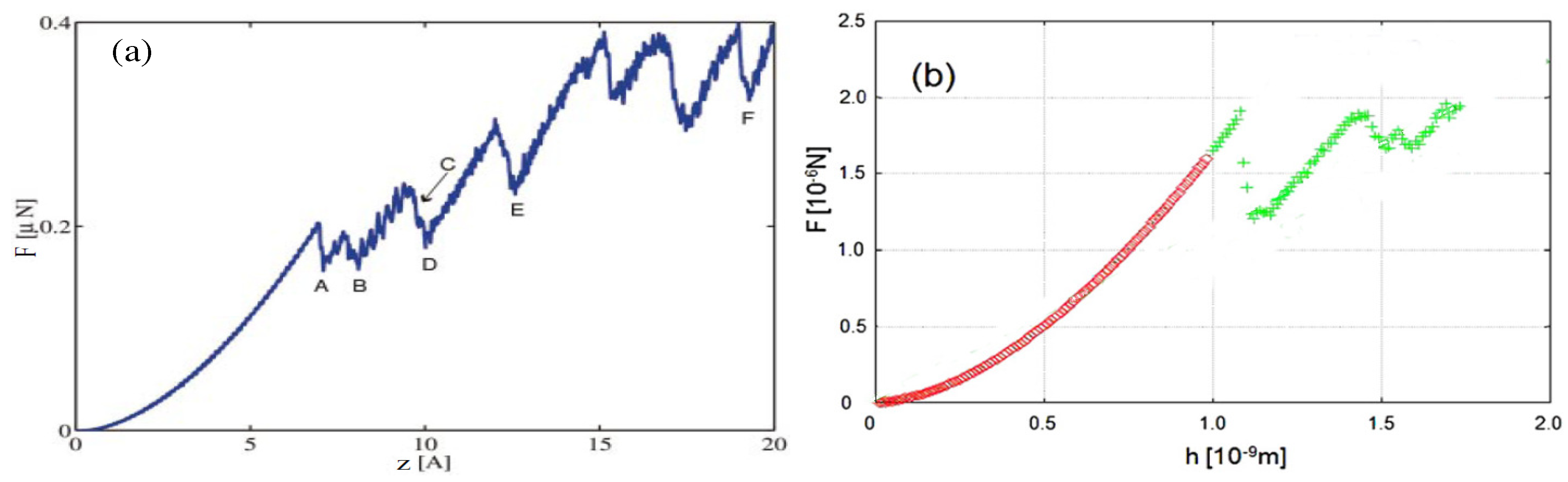
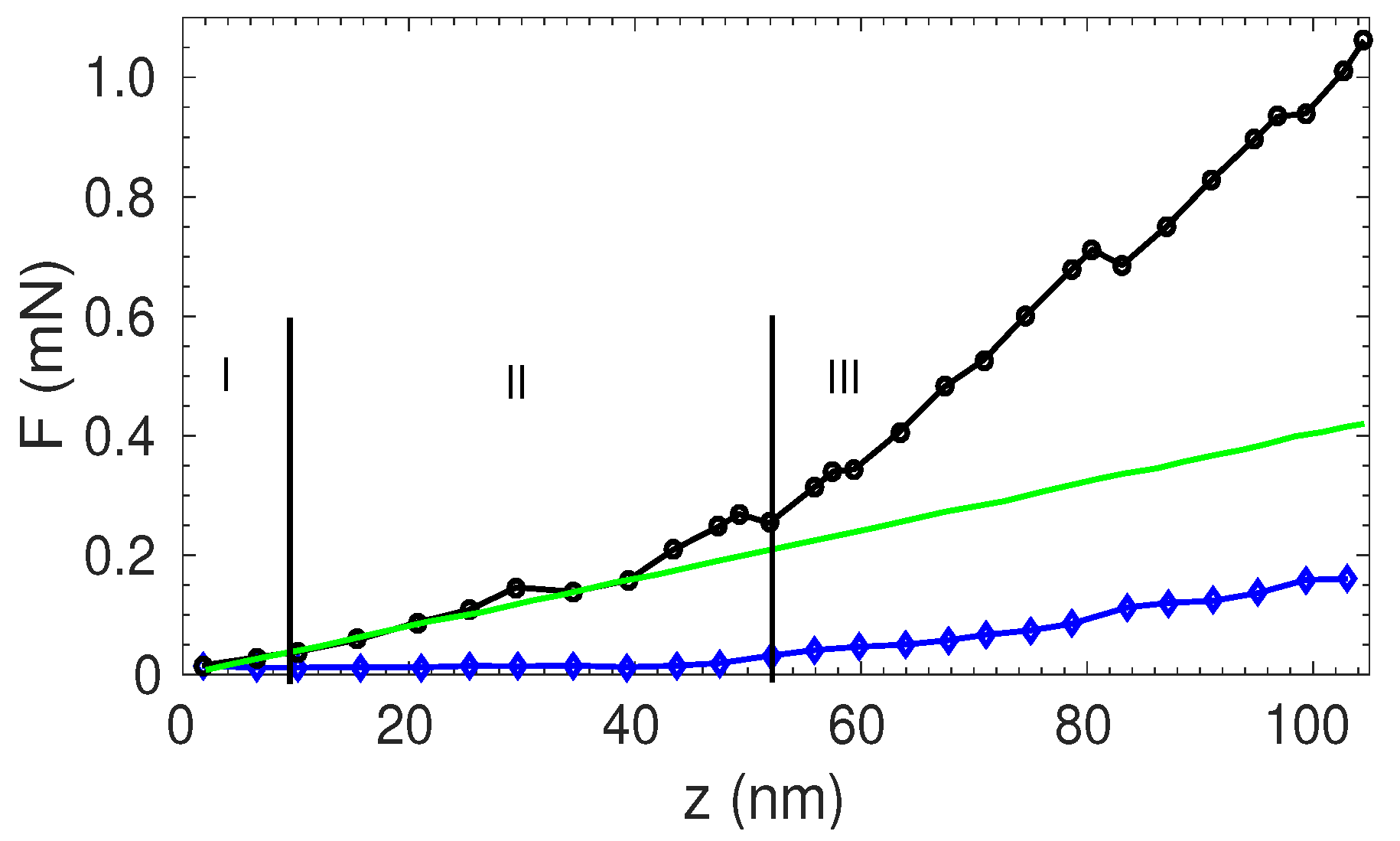
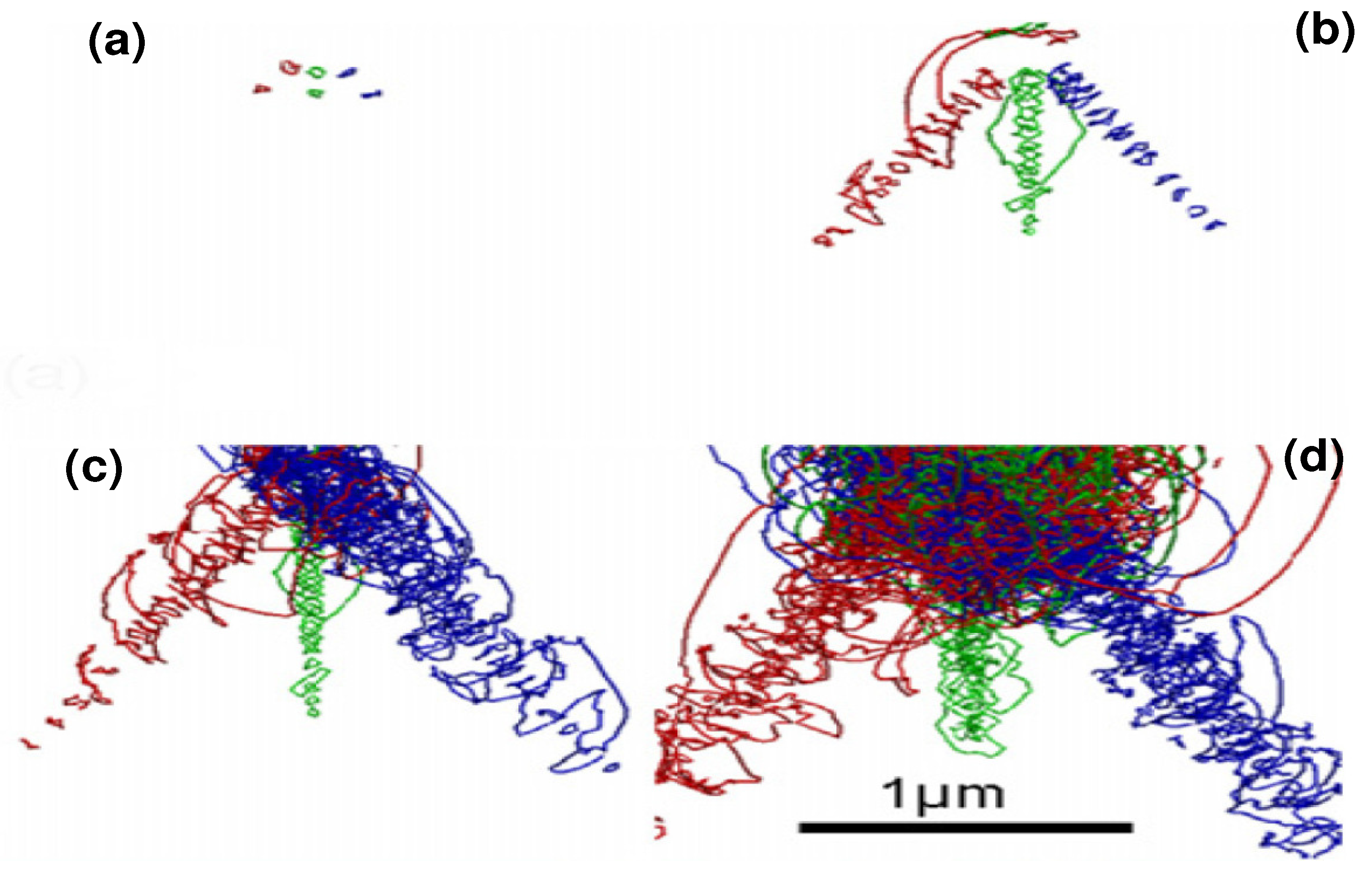
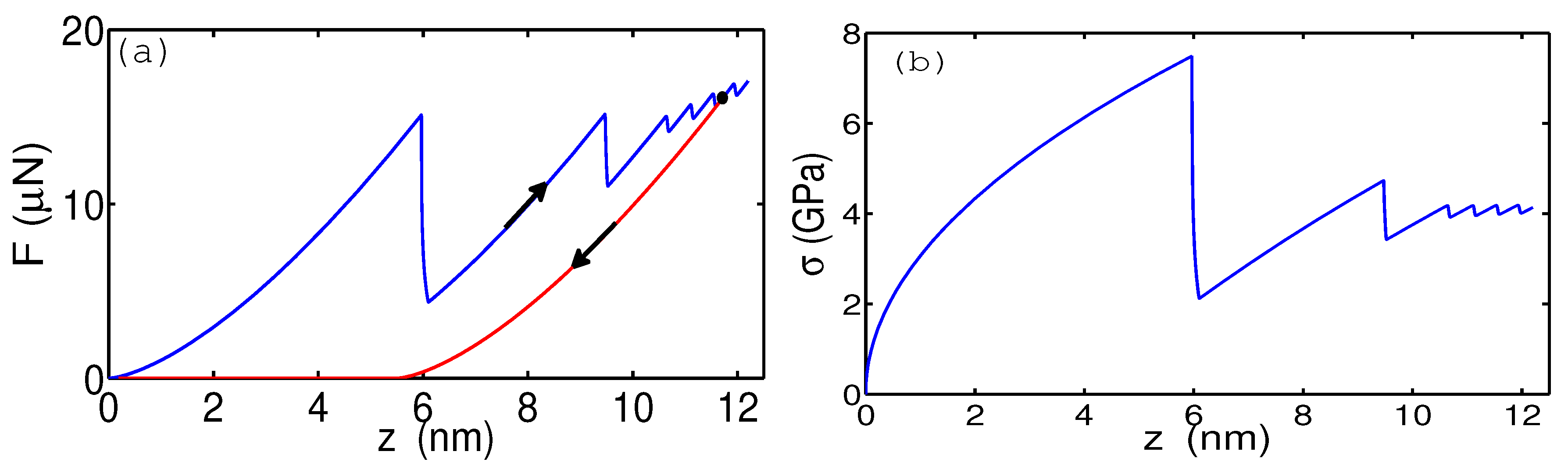
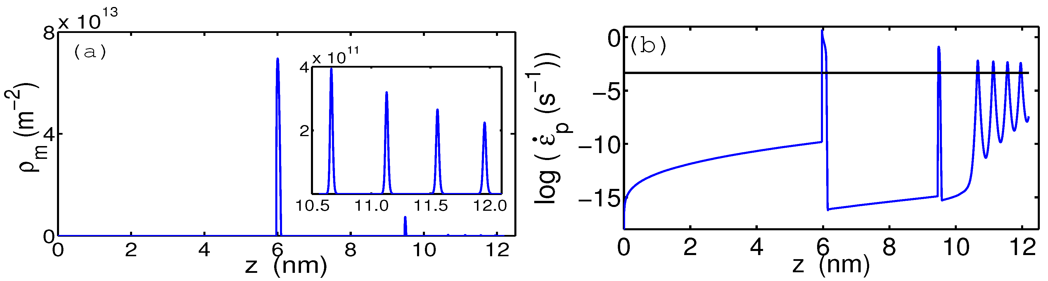
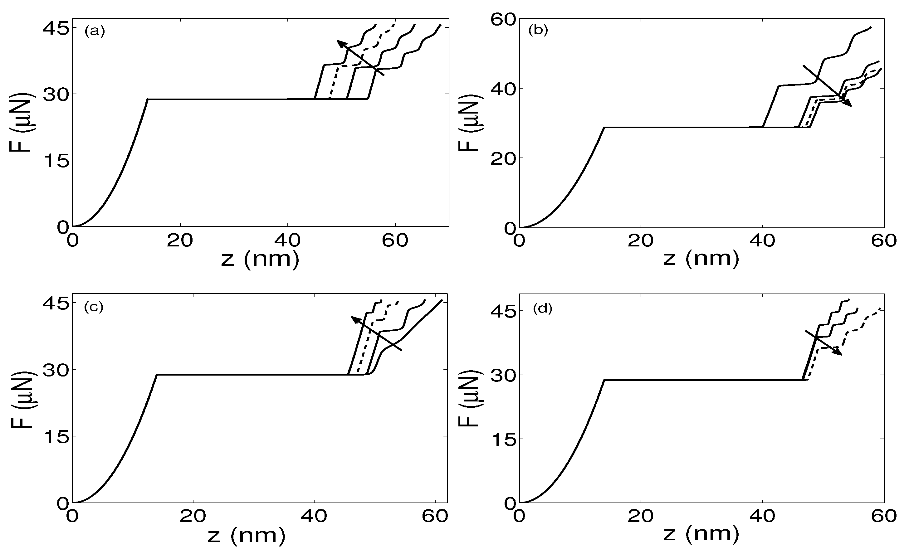
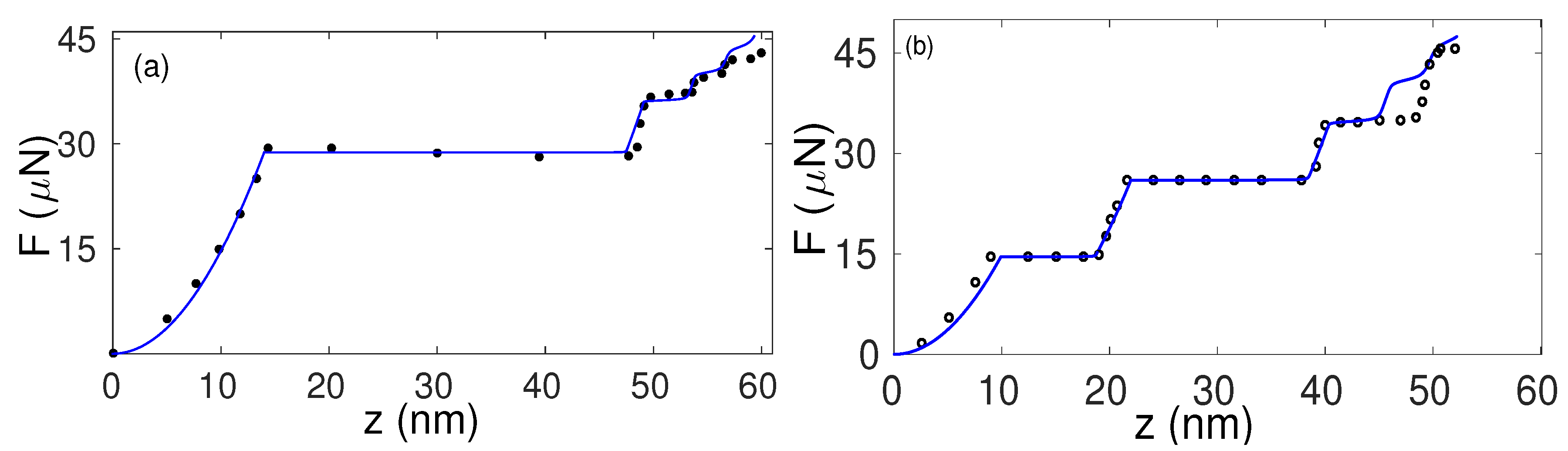
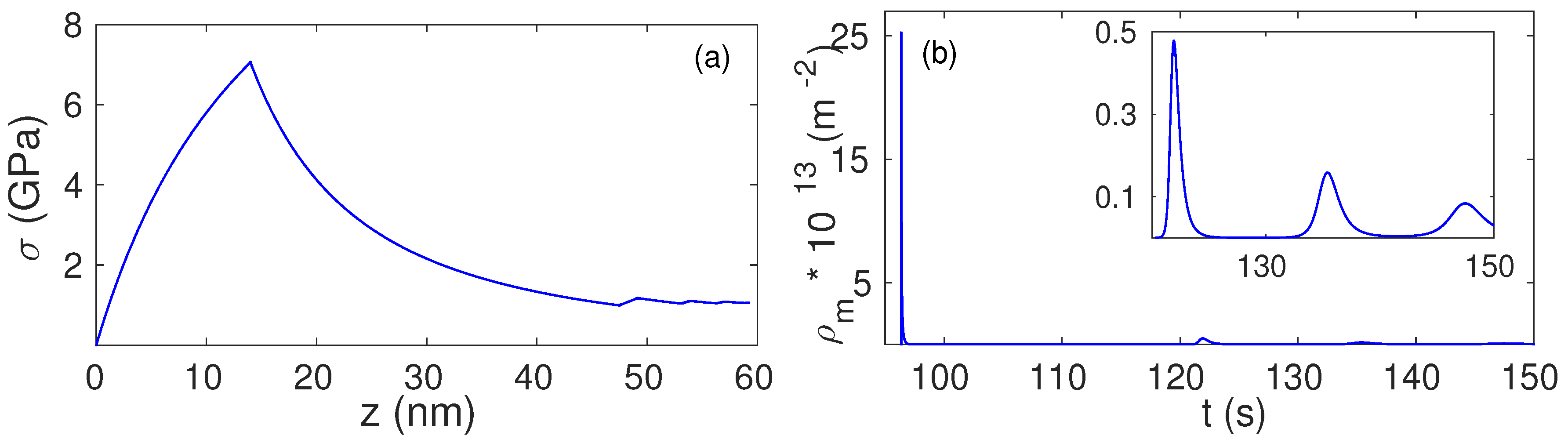
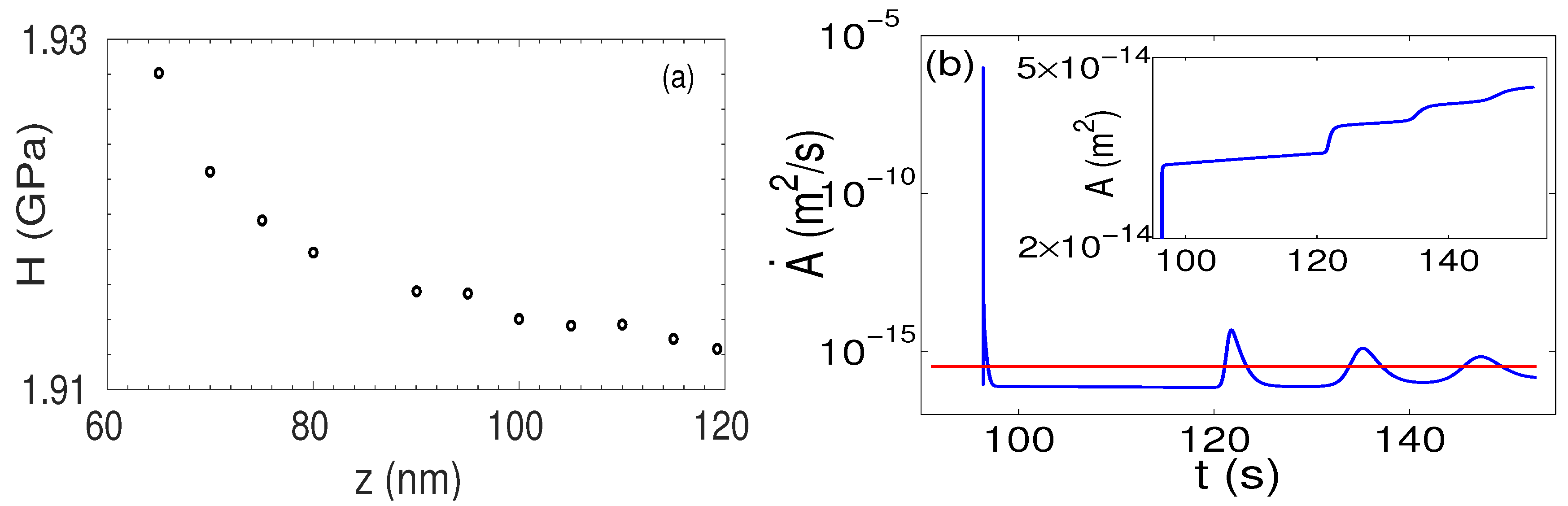
Table 1.
Parameter values used for the model. The experimental parameters used are drawn from experiments on single crystals of Au [11].
Table 1.
Parameter values used for the model. The experimental parameters used are drawn from experiments on single crystals of Au [11].
| (GPa) | (GPa) | (GPa) | (GPa) | (m/s) |
| 75 | ||||
| (Å/s) | (Å) | (m/s) | (m/s) | |
| 1075 |
Table 2.
Range of parameter values in the model equations using Berkovich indenter keeping the nominal tip radius nm and GPa.
Table 2.
Range of parameter values in the model equations using Berkovich indenter keeping the nominal tip radius nm and GPa.
| (GPa) | (GPa) | (GPa) | (N/s) |
| (m/s) | (m/s) | (m/s) | |
| 10–5 × 10 | (0.01–4) × 10 | –10 |
Table 3.
Optimized parameter values used for obtaining the best fit with the experimental load–displacement curve for single crystals of orientation [12]. Other parameters are fixed at and . Although the parameters and p have little influence on the model curves, the values cited are the values used for numerical fit with the experiment.
| (GPa) | (m/s) | p | (m/s) | (m/s) | f |
|---|---|---|---|---|---|
| 4 | 10 |
© 2018 by the authors. Licensee MDPI, Basel, Switzerland. This article is an open access article distributed under the terms and conditions of the Creative Commons Attribution (CC BY) license (http://creativecommons.org/licenses/by/4.0/).
Share and Cite
MDPI and ACS Style
Ananthakrishna, G.; Krishnamoorthy, S. A Novel Approach to Modelling Nanoindentation Instabilities. Crystals 2018, 8, 200. https://0-doi-org.brum.beds.ac.uk/10.3390/cryst8050200
AMA Style
Ananthakrishna G, Krishnamoorthy S. A Novel Approach to Modelling Nanoindentation Instabilities. Crystals. 2018; 8(5):200. https://0-doi-org.brum.beds.ac.uk/10.3390/cryst8050200
Chicago/Turabian StyleAnanthakrishna, Garani, and Srikanth Krishnamoorthy. 2018. "A Novel Approach to Modelling Nanoindentation Instabilities" Crystals 8, no. 5: 200. https://0-doi-org.brum.beds.ac.uk/10.3390/cryst8050200
Note that from the first issue of 2016, this journal uses article numbers instead of page numbers. See further details here.