On Linear and Circular Approach to GPS Data Processing: Analyses of the Horizontal Positioning Deviations Based on the Adriatic Region IGS Observables

Abstract

Global and regional positional accuracy assessment is of the highest importance for any satellite navigation system, including the Global Positioning System (GPS). Although positioning error can be expressed as a vector quantity with direction and magnitude, most of the research focuses on error magnitude only. The positional accuracy can be evaluated in terms of navigational quadrants as further refinement of error distribution, as it was shown here. This research was conducted in the wider area of the Northern Adriatic Region, employing the International Global Navigation Satellite Systems (GNSS) Service (IGS) data and products. Similarities of positional accuracy and deviations distributions for Single Point Positioning (SPP) were addressed in terms of magnitudes. Data were analyzed during the 11-day period. Linear and circular statistical methods were used to quantify regional positional accuracy and error behavior. This was conducted in terms of both scalar and vector values, with assessment of the underlying probability distributions. Navigational quadrantal positioning error subset analysis was carried out. Similarity in the positional accuracy and positioning deviations behavior, with uneven positional distribution between quadrants, indicated the directionality of the total positioning error. The underlying distributions for latitude and longitude deviations followed approximately normal distributions, while the radius was approximated by the Rayleigh distribution. The Weibull and gamma distributions were considered, as well. Possible causes of the analyzed positioning deviations were not investigated, but the ultimate positioning products were obtained as in standard, single-frequency positioning scenarios.

1. Introduction and Background

Whether it is expressed as predictable, repeatable, or relative, positioning accuracy [1] can be defined as a difference between true and measured position. The positioning error is of unreserved importance for the overall performance of Global Navigation Satellite Systems (GNSS). The total positioning error budget comprises User Equivalent Range Error (UERE), referring to positional error measurements and Dilution of Position (DOP), as an error effect due to the satellite geometry [2].

σ = UERE × DOP.

(1)

In terms of error values or positioning deviations, the satellite positioning accuracy can be expressed in numerous measures. Linear measures, such as Northing and Easting errors in meters in Universal Transverse Mercator (UTM), are commonly used [3]. Likewise, one-dimensional Root Mean Square (RMS) error in meters, two-dimensional RMS (DRMS), twice distance value of two-dimensional RMS (2DRMS) are used, the latter being the most common measure for navigational purposes. Based on probability distributions, there are two-dimensional measures, such as Circular Error Probable (CEP), Radius 95% (R95), or Radius 68% (R68) [4]. CEP is defined as the minimum circle value in which 50% of positions (measurements) are included or as radius of equal probability circle [5]. For 2DRMS, the probability varies from 95% to 98%, depending on the elongation of the error ellipse [1]. Furthermore, there is no constant relationship between 2DRMS and CEP [6,7]. Finally, for three-dimensional solutions, there are 3D equivalents, such as DRMS (3D) or Spherical Error Probable (SEP) [8].

Besides the previously stated measures, which express displacement from true position as a magnitude solely, errors can be represented as the position error vectors in the polar coordinate system, comprising of both magnitude and direction.

Circular or directional statistics methods have been developed for the assessment of directional or periodical measurements and occurrences and are used in various disciplines, such as geodesy, geophysics, geology, meteorology, and oceanography [9,10]. Such data can be represented as a point on the circumference on a unit circle, expressed as angles, and measured in both clockwise and anti-clockwise direction. The measurements taken from the origin, also referred to as zero direction, e.g., North (000° or 360°), are positive and increase when moving away from the example origin (North). This is contrary to linear values, which can be positive or negative. However, since the choice of origin and direction is arbitrary [11], the observed directional values differ in mathematical disciplines and in navigation science.

Certain circular methods focus on unitary circle and unitary vectors solely, while varieties of applications require joint usage of both directional and linear components [9,12,13,14]. Therefore, angular and linear values can be analyzed independently or jointly.

In the context of satellite positioning, circular statistics have been considered in several scientific fields, specifically positional accuracy of spatial data of satellite imagery [15], spatial uncertainty [16], GNSS-Reflectometry (GNSS-R), phase altimetry [17], and GNSS Carrier Phase Observations [10]. However, none of them dealt with the satellite positioning analysis and the positioning performance assessment.

Various satellite positioning analyses have been conducted in the Northern Adriatic area. Similarities in satellite positioning performance behavior between selected regional stations were confirmed in Reference [18]. Positional deviation and error behavior between regional stations during geomagnetic events were considered, as well [19], providing more precise understanding in satellite positioning errors’ distribution on a particular area.

The aim of the proposed research was to gain insights into the distribution of positioning deviations as derived from linear and circular analyses. The analyses employed position observables from three International GNSS Service (IGS) stations in the area. Apart from the evaluation of positioning deviation errors and underlying probability distributions, the motivation for the research was to evaluate the navigational quadrant positioning deviations and the directional trends of horizontal coordinates positioning behavior. It was done in order to contribute to a more comprehensive evaluation of satellite positioning error distribution.

In the current chapter, brief introduction and main elements of the conducted research were provided, together with established terms referring to statistical approach to the topic. The research methodology is described in the following chapter, comprising of both spatial and specific statistical segments. The results were presented and discussed further, emphasizing and discussing the main observations. In the conclusion section, the findings are summarized referring to insights into the behavior of positioning deviations.

2. Data Sources, Processing of Data and Methods

The presented analyses are based on GNSS/Global Positioning System (GPS) observables post-processing and consequent geographical coordinates deviations, as observed and calculated at three IGS Northern Adriatic locations; Graz, Padova, and Medicina [20] (Figure 1 and

Table 1. Reference locations of employed International Global Navigation Satellite Systems (GNSS) Service (IGS) stations.

	IGS Graz	IGS Padova	IGS Medicina
Site Code	GRAZ00AUT	PADO00ITA	MEDI00ITA
Latitude	47.067° N	45.411° N	44.520° N
Longitude	15.493° E	11.896° E	11.647° E
Height	538.3 m	64.7 m	50.0 m

, respectively).

The initial datasets were retrieved from the IGS, in the form of Receiver Independent Exchange Format observation (RINEX.d) and navigation (RINEX.n) files [21,22]. The positioning solutions were calculated according to the standard Single Point Positioning (SPP) process.

The ionospheric delay was modeled using the standard ionospheric correction model employing the broadcasted coefficients within the GPS navigational message [23]. The elevation mask angle was set to 15° to minimize the effect of the satellite geometry. The solution format was expressed in latitude, longitude, and height, respectively. The Saastamoinen model [24] was employed for the correction of the tropospheric delay. The position resolution frequency was set to 60 s. The defined satellite positioning scenario was considered to represent a standard solution obtained with single-frequency satellite positioning receivers, using a standard positioning algorithm.

The analyzed data covered the period from 10 March 2017 00:00 UTC to 20 March 2017 UTC 23:59. The reference, horizontal positions used as station coordinates origins were defined as an average of respective weekly positions [25], with their values presented in

Table 2. IGS stations horizontal coordinates origins.

	GRAZ00AUT		PADO00ITA		MEDI00ITA
GPS Week	Latitude	Longitude	Latitude	Longitude	Latitude	Longitude
1939	47.067131694	15.493483758	45.411155497	11.896065219	44.519959237	11.646818294
1940	47.067131700	15.493483762	45.411155506	11.896065216	44.519959243	11.646818289
1941	47.067131696	15.493483763	45.411155502	11.896065220	44.519959237	11.646818290
Average	47.067131697	15.493483761	45.411155502	11.896065218	44.519959239	11.646818291

.

The deviations of latitude and longitude geographical coordinates were calculated as a difference between positioning solutions and averaged combined weekly station positions representing coordinate origin, expressed in meters. Respective horizontal positioning errors were calculated as Euclidean distances in meters. Positions throughout the observation period were further divided into subsets and distributed quadrantally and clockwise, with true north as zero (reference) direction. With absolute stations geographical coordinates as a center origin, the surrounding areas were divided by four cardinal directions, with clockwise orientation as navigational quadrants: North (I), East (II), South (III), and West (IV) (Figure 2).

For data segmentation and positioning deviations presentation, the nearest neighbor calculation algorithm with Euclidian distances between points was used, presented here with a general equation [26]:

$$dist\left(x,y\right)=\sqrt{{{\displaystyle \sum }}_{i=1}^n{\left(x_i-y_i\right)}^2}.$$

(2)

The distance threshold to consider two neighboring points as neighbors (smoothing bandwidth) can be adjusted, with default value of 0.5. The default bandwidth $h$ is based on normal distribution approximation or Silverman’s rule of thumb which can be expressed as [26]:

$$h=0.9\min \left(SD, \frac{IQR}{1.34}\right)n^{-\frac{1}{5}},$$

(3)

with Standard Deviation $\left(SD\right)$, interquartile range $\left(IQR\right)$, and $n$ as the number of samples.

Coordinate deviations were further converted from the Cartesian to polar coordinate system, to render directional analysis possible. In the polar coordinate system, coordinates are represented by radius (r) and angle-theta (θ). In navigation science, azimuth (ω) is the calculated angle from the true north in the polar coordinate system. Since the distributions are considered as in navigational quadrants, ω was used instead of θ. Once transformed, these values were expressed as radius vectors defined by radius in meters, and azimuth measured from true north in degrees. The basic formulas are presented below.

$$\mathrm{r}= \sqrt{{\mathrm{d}}_{\mathrm{lon}}{}^2+{\mathrm{d}}_{\mathrm{lat}}{}^2}.$$

(4)

The lowercase letter d represents latitude and longitude deviations from true station coordinates. Respective value of radius r is, therefore, calculated as a square root of squared latitude and longitude deviations.

$${\tan }^{-1}\mathsf{\omega }= \frac{{\mathrm{d}}_{\mathrm{lon}}}{{\mathrm{d}}_{\mathrm{lat}}}.$$

(5)

All $\mathsf{\omega }$ values were converted to their true format in the polar coordinate system (0° to 360°).

The assessment of the underlying latitude and longitude deviation distributions was performed, analyzed, and correlated. Radius distributions were considered as follows, with the assessment and possible curve fittings for candidate distributions.

Radius distribution data were fitted using different univariate distributions, assuming that samples are independent and identically distributed. The distribution parameters θ are by default estimated by maximizing the likelihood function, which is defined as [27]:

$$L\left(\theta \right)={\displaystyle \prod }_{i=1}^{n}f\left(x_i|\theta \right),$$

(6)

with $x_i$ the $n$ observations of variable $X$, and $f(.|\theta )$ as the density function of the parametric distribution.

The analyzed period was assessed in terms of geomagnetic activity and, based on the planetary K_p index observables, interpreted as quiet [28,29] (Figure 3).

Positioning solutions were calculated with the RTKLIB: An Open Source Program Package for GNSS Positioning, employing an iterative weighted Least Square Estimation (LSE) for the SPP [30,31]. The analyses were carried out using R statistical language version 3.6.3. with RStudio 1.2.5033 and several contribution packages [13,26,32,33].

3. Results

The data were first analyzed in the Cartesian coordinate system for all navigational quadrants, and subsequently for each navigational quadrant separately. A combined circular and linear analyses in polar coordinate system are presented as follows.

3.1. Quadrantal Analysis in the Cartesian Coordinate System

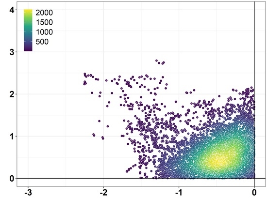
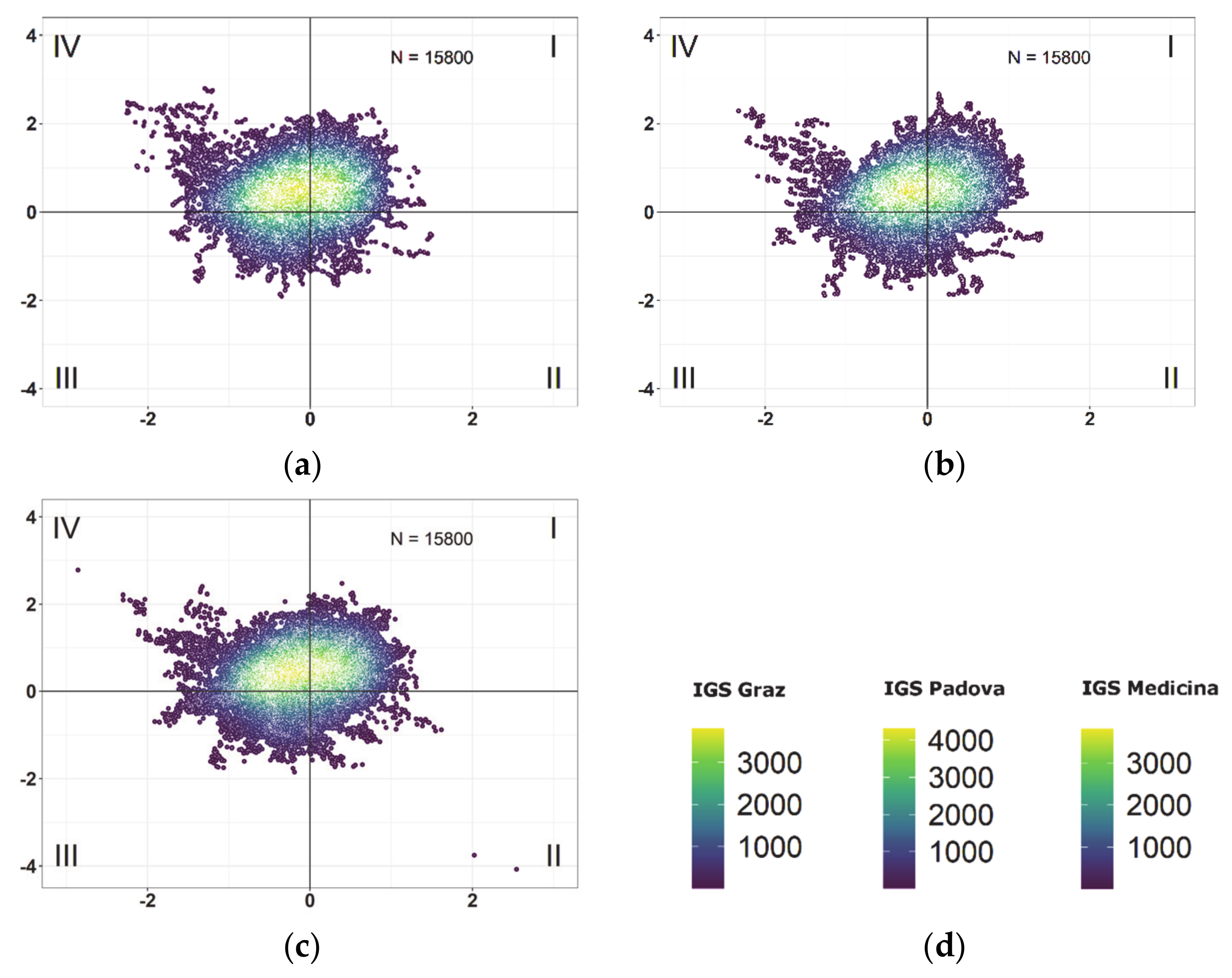
Positions (deviations) were distributed unevenly between the northern (I, IV) and the southern quadrants (II, III), with higher density in northward direction. The latitude and longitude spread, and the range can be seen in Figure 4.

The highest distribution density was present in the navigational quadrant IV, as observed on all locations. The position spread was mostly elliptical, extending roughly longitudinally from coordinate origin towards E and W to the navigational quadrants I and IV. There was a prominent northwest (NW) arm extending from the origin to the NW corner of the navigational quadrant IV, observable in all distributions. Generally, the most compact distribution shape was present at IGS Graz. The density scale on respective figures is relative to each station positioning deviation distributions.

Statistical summary for all four navigational quadrants was termed as the full circle summary. The ranges and Inter Quartile Ranges (IQR) were approximately similar for all deviations, with the exception of latitude range for IGS Medicina (

Table 3. Full circle summary statistics for latitude and longitude deviations (m).

	Minimum		Q1		Median		Mean		Q3		Maximum		IQR		SD
	Lat	Lon	Lat	Lon	Lat	Lon	Lat	Lon	Lat	Lon	Lat	Lon	Lat	Lon	Lat	Lon
GRAZ	−1.91	−2.26	0.00	−0.53	0.41	−0.15	0.40	−0.16	0.82	0.26	2.79	1.50	0.82	0.78	0.65	0.55
PADO	−1.89	−2.33	0.04	−0.50	0.44	−0.13	0.42	−0.14	0.82	0.25	2.67	1.40	0.78	0.75	0.64	0.54
MEDI	−4.07	−2.86	0.00	−0.51	0.40	−0.12	0.38	−0.14	0.27	0.27	2.78	2.54	0.80	0.78	0.64	0.55

). The value was the single largest latitude error of 4.07 m, being an outlier falling below the lower outer fence (Q1 − 3 × IQR). Abbreviations Q1 and Q3 denote Quartile 1 and Quartile 3, while SD stands for Standard Deviation.

Conversely, individual latitude and longitude deviation median, mean and standard deviation values were similar. Moreover, median and mean values were relatively close, indicating approximate symmetry.

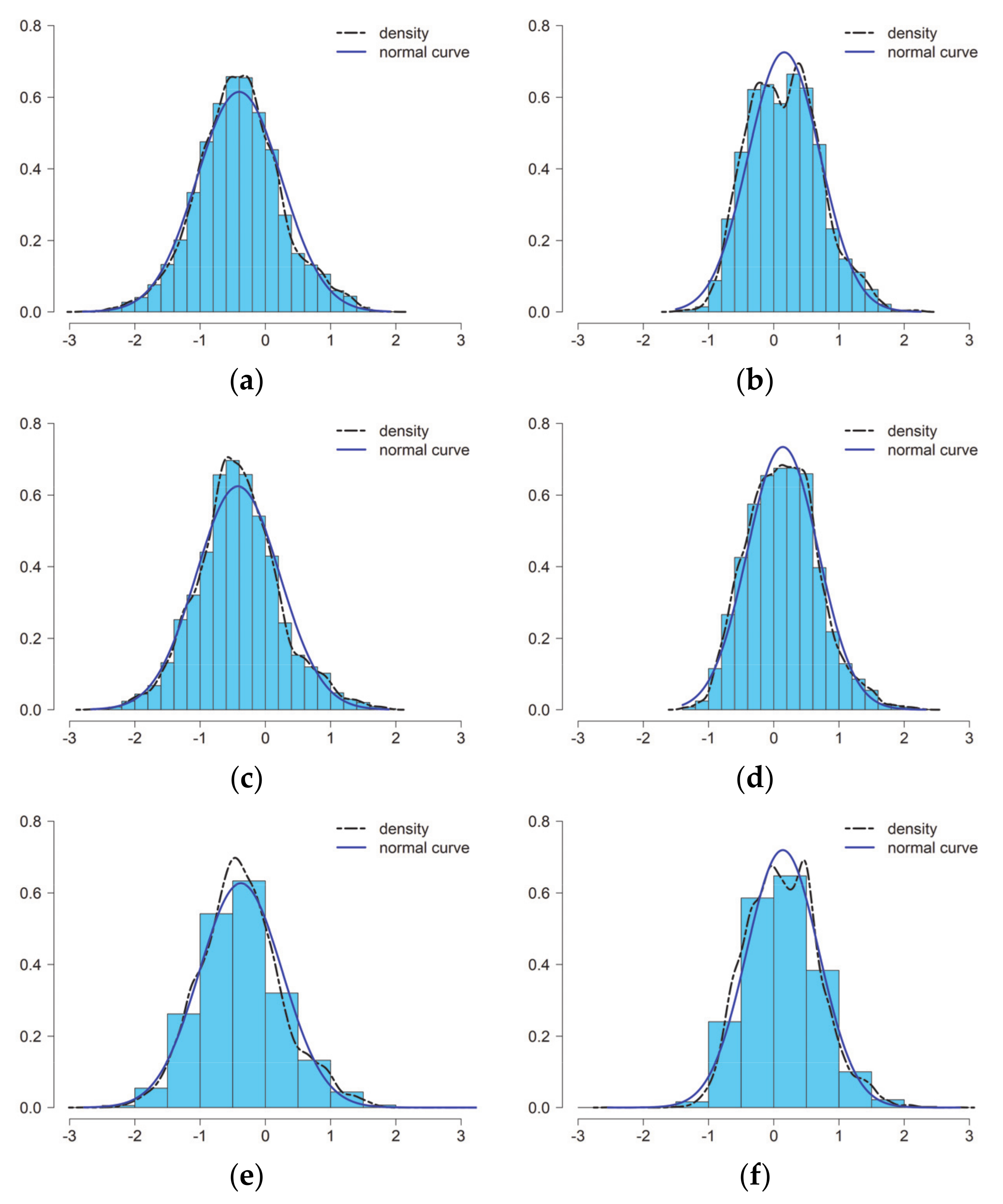
The underlying distributions were assessed with results presented in Figure 5.

Both latitude and longitude deviations follow a roughly normal distribution with a certain departure from normality. Although visual assessment of histogram supports an approximation of normality, skewness and tails are also evident. Likewise, some flatness and irregularities of the longitude deviations, higher peaks of the latitude deviations, compared to normal distribution are observed.

The distributions were analyzed by using quantile-quantile (Q-Q) plots, on which departures from normality in tails of the distributions were visible. To further assess the distributions, kurtosis and skewness values were calculated, as presented in

Table 4. Skewness and kurtosis values for latitude and longitude deviations distributions.

	Graz		Padova		Medicina
	Lat	Lon	Lat	Lon	Lat	Lon
Skewness	−0.11	0.30	−0.23	−0.31	0.31	−0.29
Kurtosis	3.28	2.84	3.46	3.10	3.44	3.05

.

Skewness and kurtosis are third and fourth moments of a distribution after location and variability. Kurtosis indicates tailedness or tail extremity of the distribution [34], with higher values indicating outliers. Kurtosis value for standard normal distribution is 3, however sometimes it is stated as 0 because the value of 3 is subtracted. This is referred as the excess kurtosis. Skewness indicates departure from distribution symmetry, with value of 0 for the standard normal distribution.

Besides observational techniques and descriptive analysis, normality can be assessed with formal tests, such as Anderson-Darling, Kolmogorov–Smirnov, or Shapiro-Wilk, to name a few. The results and acceptance of null hypothesis of normality are method and sample size dependent. With large sample size or even whole datasets analysis, the hypothesis of normality is commonly rejected [35]. This was the case with the presented data since the whole dataset was analyzed instead of random sampling. The skewness and kurtosis values were also used to assess normality, as it is presented in Reference [36]. Skew values larger than 2 and kurtosis values larger than 7 can be considered as substantial departure from normality. As presented in Table 4 and in Figure 5, latitude and longitude deviation distributions are not substantially non-normal. Finally, correlation was assessed using Pearson’s correlation between latitude and longitude deviations resulting with very weak positive correlation results of 0.11 for IGS Graz, 0.16 for IGS Padova, and 0.16 for IGS Medicina. This was carried out to assess the randomness and uncorrelation assumption required for the candidate Rayleigh distribution. The obtained results are lower than the correlation values of simulated latitude and longitude errors in Reference [6].

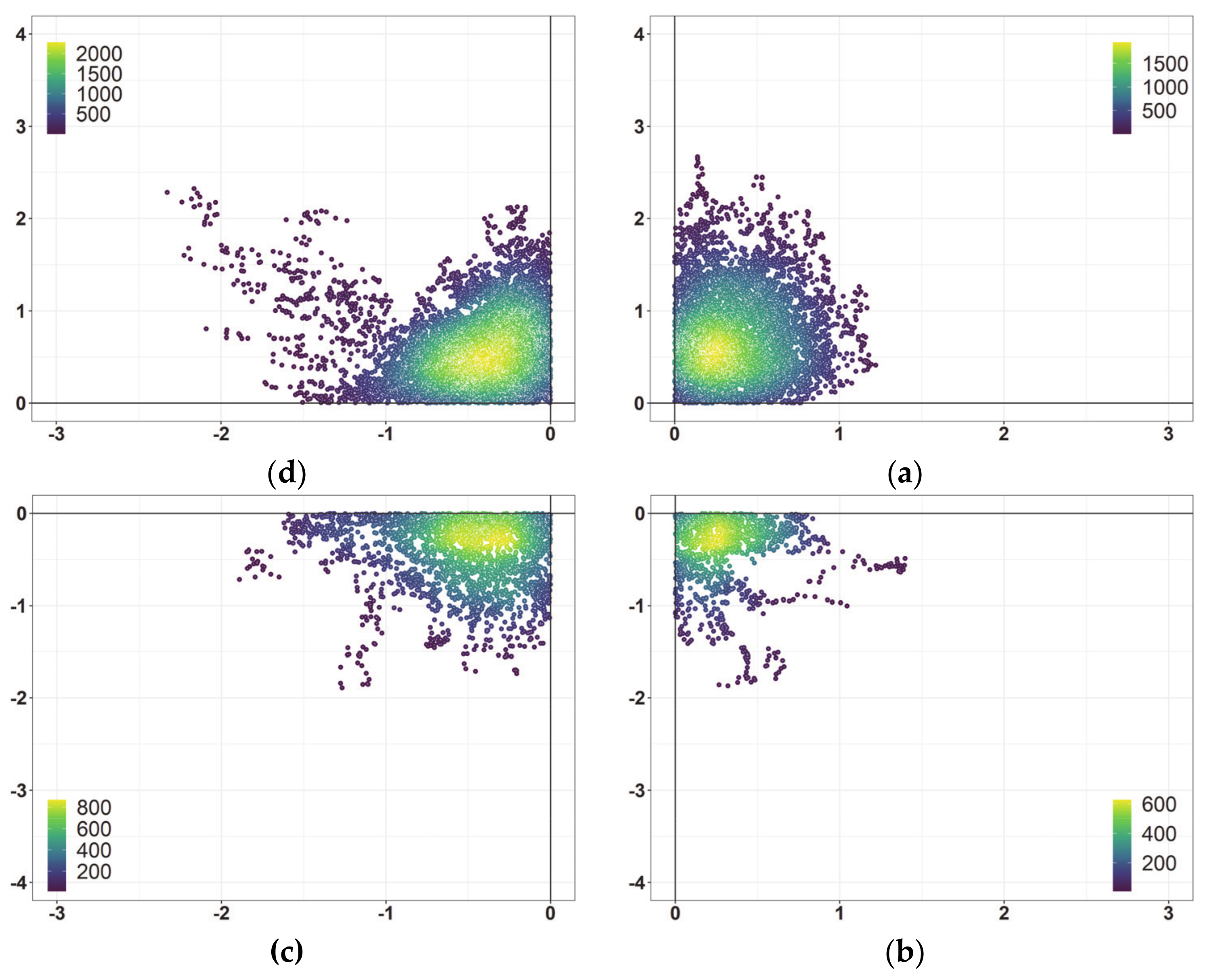
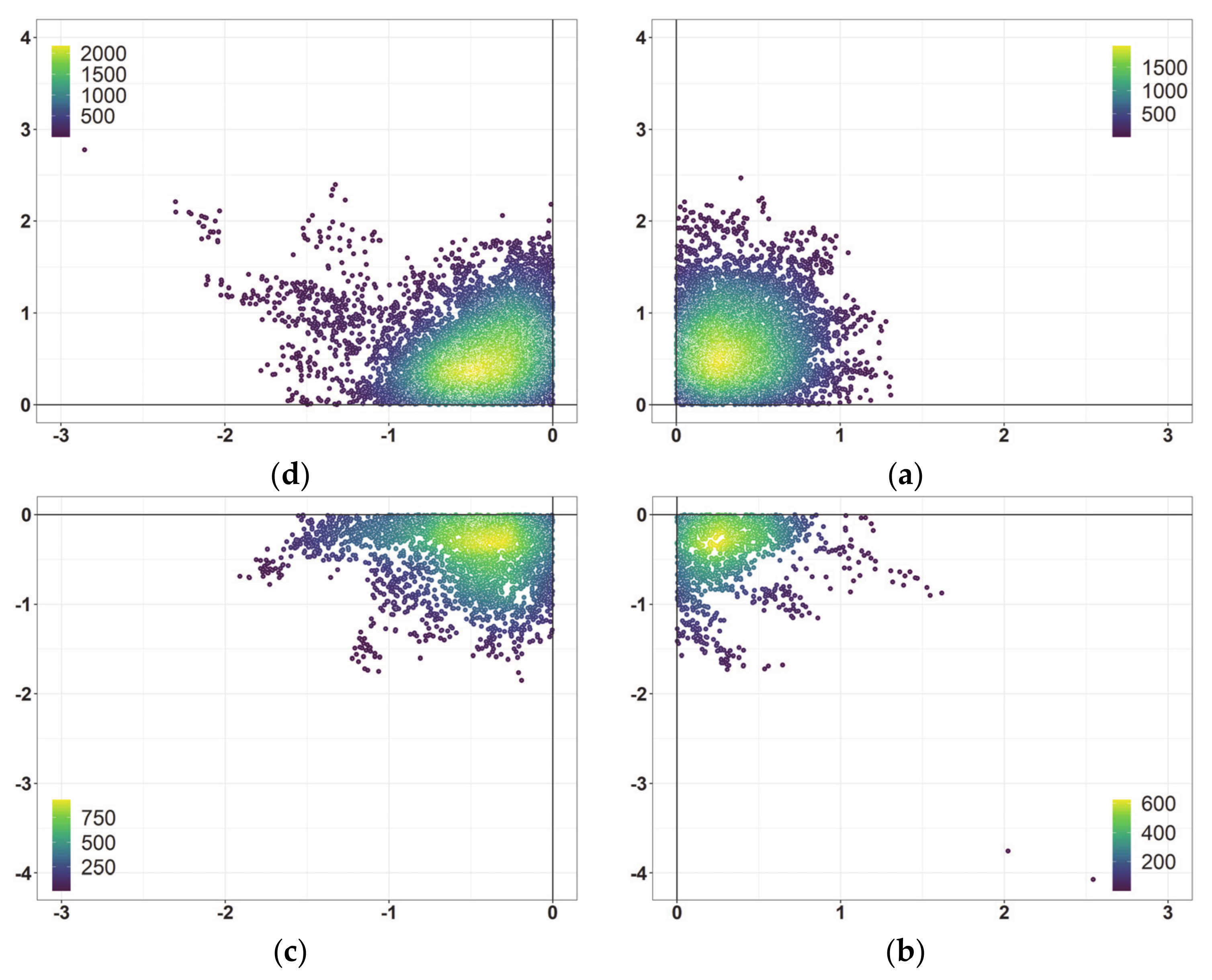
After the full circle analysis, the data in each navigational quadrant were evaluated as subsets. Again, the previously observed spread from all navigational quadrants is noticeable extending in roughly longitudinal E to W direction. The observables distribution and navigational quadrant unevenness was investigated further. Positioning deviations values in quadrantal subsets are presented in

Table 5. Summary statistics for navigational quadrants latitude and longitude deviations (in m).

	Minimum		Q1		Median		Mean		Q3		Maximum		IQR		SD
	Lat	Lon	Lat	Lon	Lat	Lon	Lat	Lon	Lat	Lon	Lat	Lon	Lat	Lon	Lat	Lon
	Navigational quadrant I
GRAZ	0.00	0.00	0.35	0.16	0.65	0.32	0.72	0.36	1.00	0.53	2.31	1.40	0.65	0.37	0.46	0.25
PADO	0.00	0.00	0.39	0.16	0.67	0.34	0.75	0.38	1.05	0.56	2.67	1.22	0.66	0.40	0.47	0.26
MEDI	0.00	0.00	0.37	0.17	0.64	0.35	0.70	0.39	1.00	0.39	2.47	1.31	0.64	0.41	0.44	0.26
	Navigational quadrant II
GRAZ	−1.65	0.00	−0.54	0.15	−0.27	0.34	−0.39	0.36	−0.12	0.50	0.00	1.50	0.42	0.34	0.36	0.25
PADO	−1.87	0.00	−0.62	0.13	−0.29	0.28	−0.43	0.33	−0.14	0.47	0.00	1.40	0.49	0.34	0.40	0.27
MEDI	−4.07	0.12	−0.66	0.12	−0.31	0.34	−0.44	0.34	−0.12	0.49	0.00	2.54	0.54	0.37	0.42	0.28
	Navigational quadrant III
GRAZ	−1.91	−1.71	−0.70	−0.74	−0.34	−0.46	−0.45	−0.53	−0.14	−0.27	0.00	0.00	0.56	0.47	0.37	0.35
PADO	−1.89	−1.89	−0.68	−0.76	−0.30	−0.48	−0.43	−0.55	−0.12	−0.26	0.00	0.00	0.56	0.49	0.38	0.39
MEDI	−1.85	−1.91	−0.70	−0.82	−0.33	−0.48	−0.45	−0.57	−0.14	−0.26	0.00	0.00	0.56	0.55	0.38	0.40
	Navigational quadrant IV
GRAZ	0.00	−2.25	0.29	−0.72	0.56	−0.46	0.64	−0.53	0.90	−0.25	2.79	0.00	0.61	0.47	0.46	0.46
PADO	0.00	−2.33	0.28	−0.65	0.56	−0.41	0.62	−0.48	0.86	−0.21	2.33	0.00	0.58	0.44	0.42	0.37
MEDI	0.00	−2.86	0.27	−0.67	0.53	−0.44	0.61	−0.49	0.87	−0.21	2.78	0.00	0.60	0.46	0.42	0.37

and Figure 6, Figure 7 and Figure 8. For consistency with full circle analysis, coordinate origins of each individual navigational quadrant were the same (0,0). Furthermore, summary statistics for individual quadrants are expressed as relative values, being either positive or negative (+/−) depending on the quadrant. This must be considered when interpreting the statistical summary results in Table 3 and Table 5, for example, maximum and minimum.

The greatest number of deviated positions is placed in the navigational quadrant IV, followed by the navigational quadrant I, the navigational quadrant III, and, finally, the navigational quadrant II. Furthermore, observing the relative densities, the highest density areas are more elliptical in the navigational quadrants III and IV. The highest density areas in the navigational quadrants I and II are of a more compact shape.

Table 5 shows the statistical summary for individual navigational quadrants. The highest absolute latitude median values were placed in the navigational quadrants I and IV, while the highest longitude median values were placed in the navigational quadrants III and IV, being the same as for the mean values. Latitude IQR is the highest in the navigational quadrants I and IV and the lowest in the navigational quadrant II, although the IQR value for Medicina in the navigational quadrant II is higher.

3.2. Linear Statistics Analysis

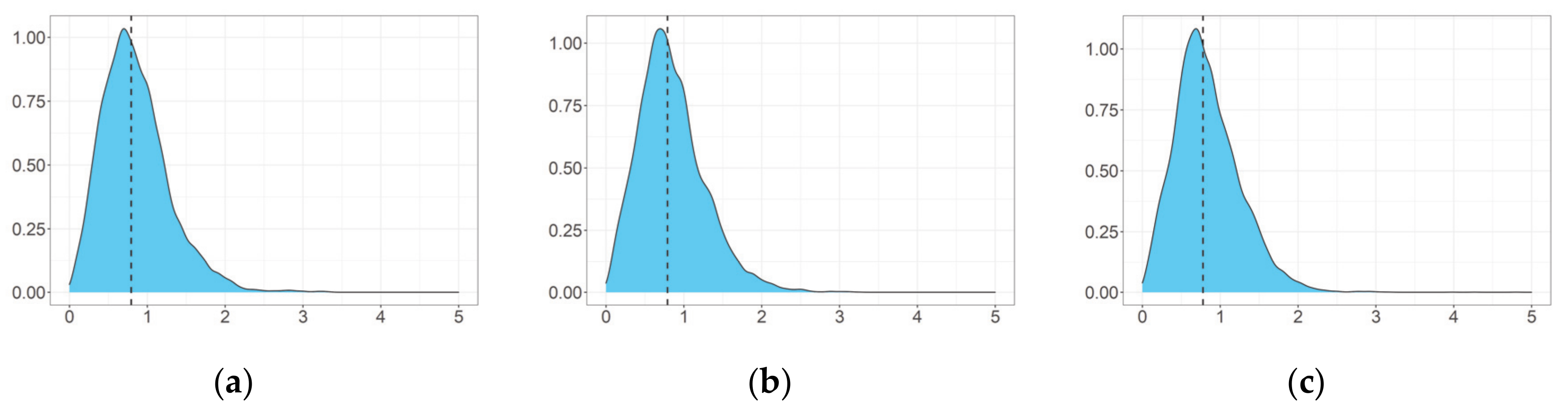
This section presents the results of radius distribution linear analysis. The obtained radius value is the error magnitude from the origin or the zero value. The radius distributions of the observed IGS stations are presented in Figure 9.

As stated above, the radius value was calculated from two independent and uncorrelated variables of latitude and longitude deviations. The result was a joint distribution from univariate latitude and longitude deviations. The radius distribution is, therefore, a cumulative distribution of the latitude and longitude deviation distributions.

Table 6. Radius linear statistics summary (m).

	Min	Q1	Med	Mean	Q3	Max	IQR	Skew 1	Kurt 1
GRAZ	0.01	0.54	0.79	0.85	1.08	3.35	0.54	1.00	1.98
PADO	0.01	0.55	0.79	0.85	1.08	3.26	0.53	0.86	1.32
MEDI	0.07	0.55	0.78	0.84	1.08	4.79	0.53	0.86	1.89

¹ dimensionless.

presents the statistical summary for linear radius values.

As presented, the orthogonal latitude and longitude coordinate distributions were approximately normal. Taking this into consideration, Rayleigh distribution is commonly stated as the underlying position deviation distribution [37] or as sufficient approximation [38].

Rayleigh distribution is a special case of Weibull distribution with shape value of 2. Among others, it is also related to gamma distribution. For the linear radius error, Rayleigh distribution was assumed, given that the component variables are random and uncorrelated [39].

In some cases, the position distribution can be approximated as a normal circular distribution [5]. In Reference [40], assumptions for Rayleigh distribution were evaluated, due to inequality of easting and northing errors and because of poor satellite visibility at higher latitudes. Likewise, in the same study, notions of GPS positioning error normality were discussed. Here, evaluation and analysis of GPS positioning errors confirmed the Rayleigh distribution approximation [40].

Rayleigh, Weibull, gamma, and normal distributions were evaluated in Reference [41], where gamma distribution was proposed as the best possible fit.

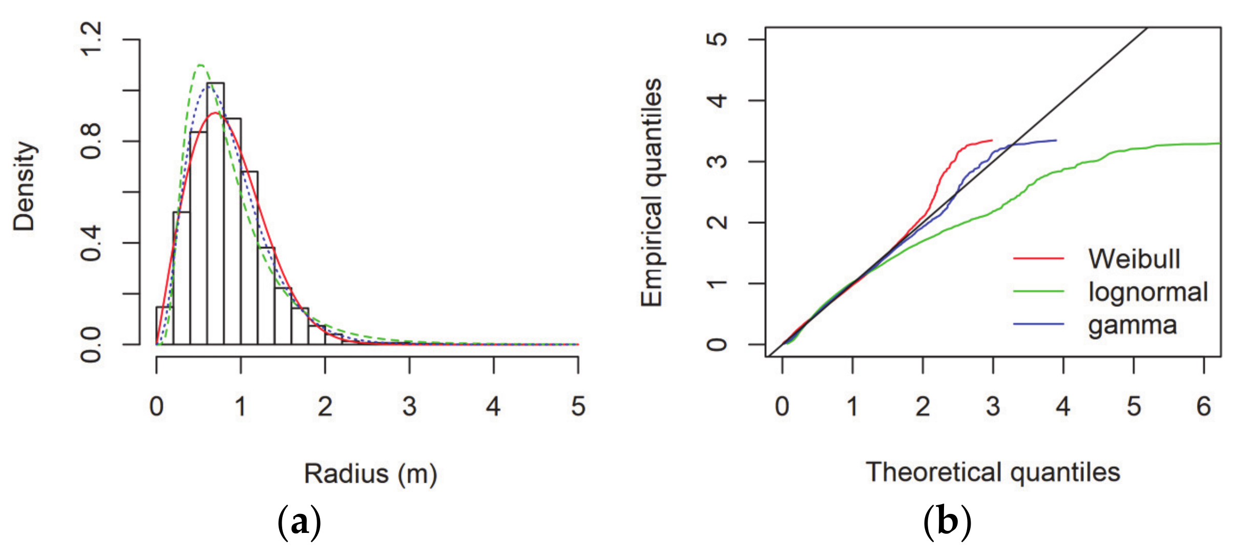
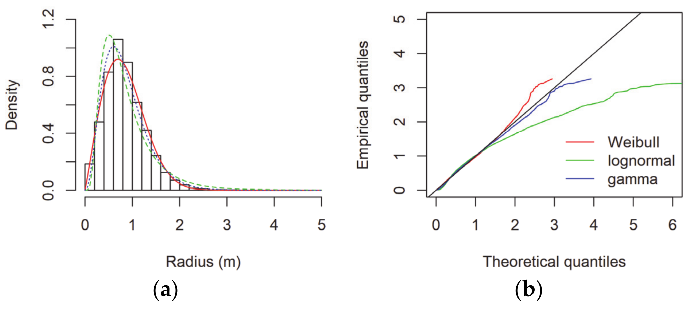
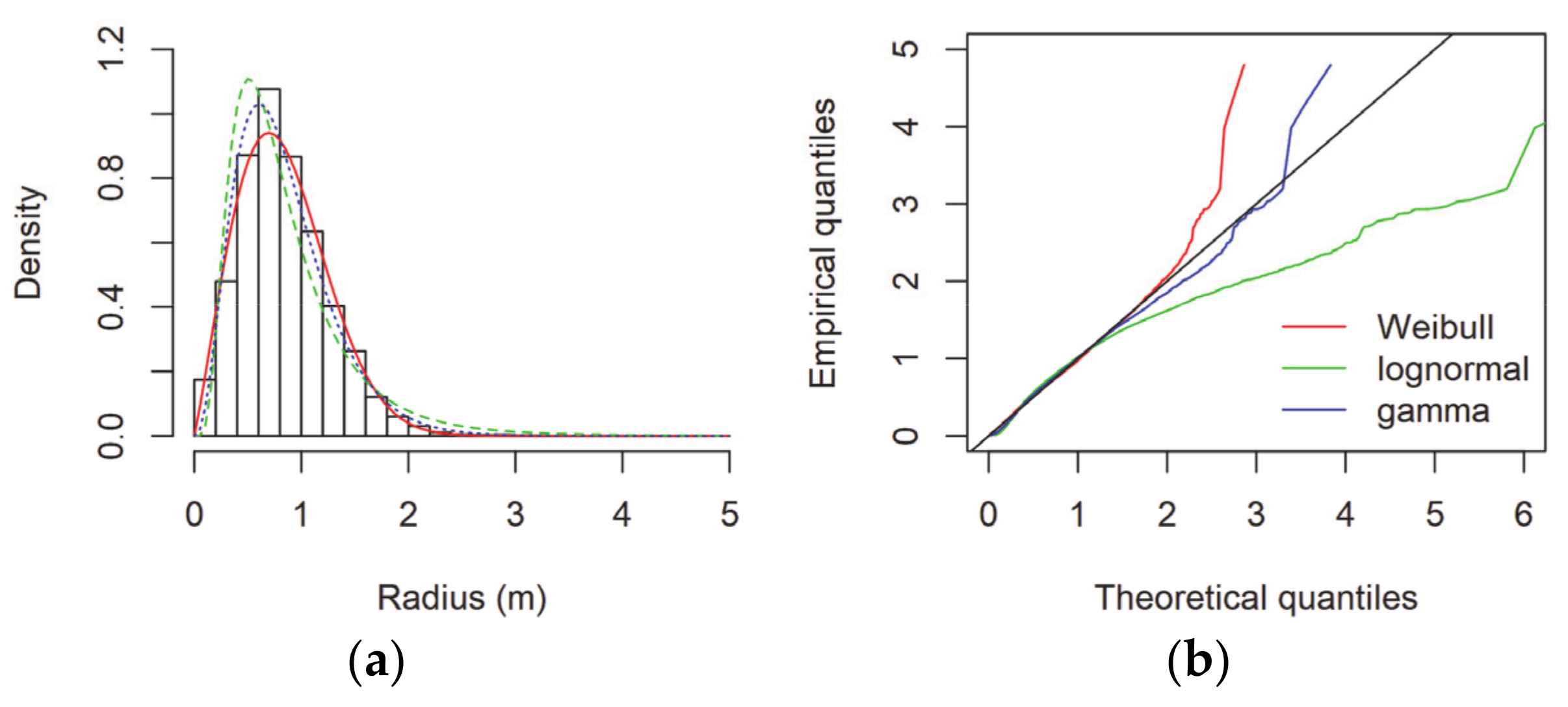
To evaluate possible fits of the radius distributions, goodness of fit evaluation tests for the selected Weibull, gamma, and lognormal distributions were conducted, employing Maximum Likelihood Estimation (MLE) method [27]. The results allowed that both Weibull and gamma distribution can be fitted to the observed data, which can be observed in Figure 10, Figure 11 and Figure 12. Furthermore, the estimated shape values for Weibull distribution were 2.06 for IGS Graz, 2.07 for IGS Padova, and 2.11 for IGS Medicina. This shape value was close to shape value of 2, which is a special case when Weibull distribution becomes Rayleigh distribution.

Goodness of fit tests for the Weibull and gamma distributions were performed, as well. The results are presented in

Table 7. Goodness of fit test results for selected radius distributions of employed IGS stations.

	Graz		Padova		Medicina
Goodness of fit statistics	Weibull	gamma	Weibull	gamma	Weibull	Gamma
Kolmogorov-Smirnov	0.03	0.03	0.03	0.04	0.03	0.03
Cramer-von Mises	4.03	3.93	3.59	5.94	2.99	5.61
Anderson-Darling	26.92	22.84	20.81	36.84	16.98	37.25
Goodness of fit criteria
Akaike’s Information Criterion	16,405.33	16,327.39	16,262.02	16,488.33	15,519.17	15,801.99
Bayesian Information Criterion	16,420.66	16,342.73	16,277.35	16,503.67	15,534.50	15,817.32

. Statistical description refers to the distance between fitted cumulative distribution function and the empirical distribution function, with a lower value representing better fit. Although these statistics should facilitate distribution selection, they are calculated differently. Methods used for these statistics assign different weights to certain parts of distributions. Therefore, these values should be interpreted cautiously, and with understanding of each test and representative results [27]. Here, the values were quite comparable; therefore, both tested distributions could be approximately fitted.

3.3. Circular Statistics Analysis

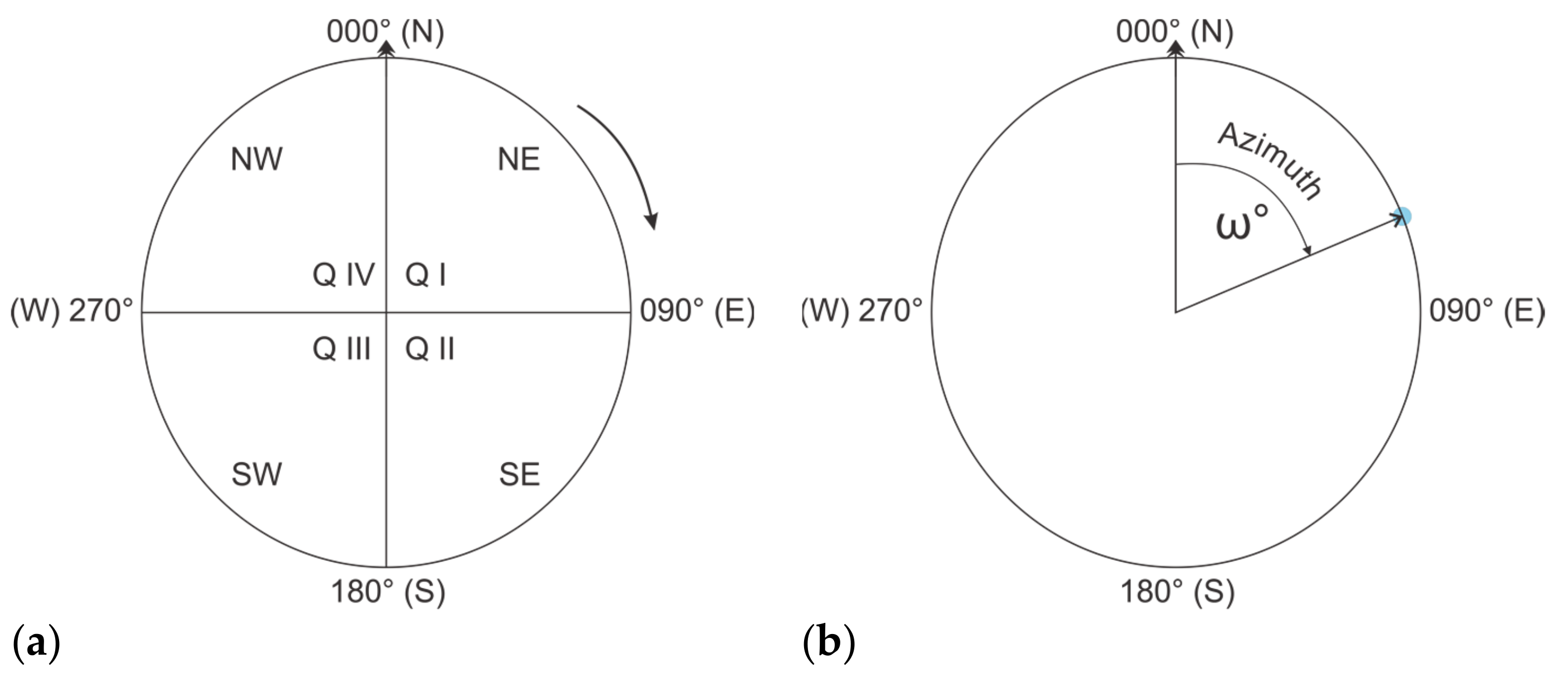
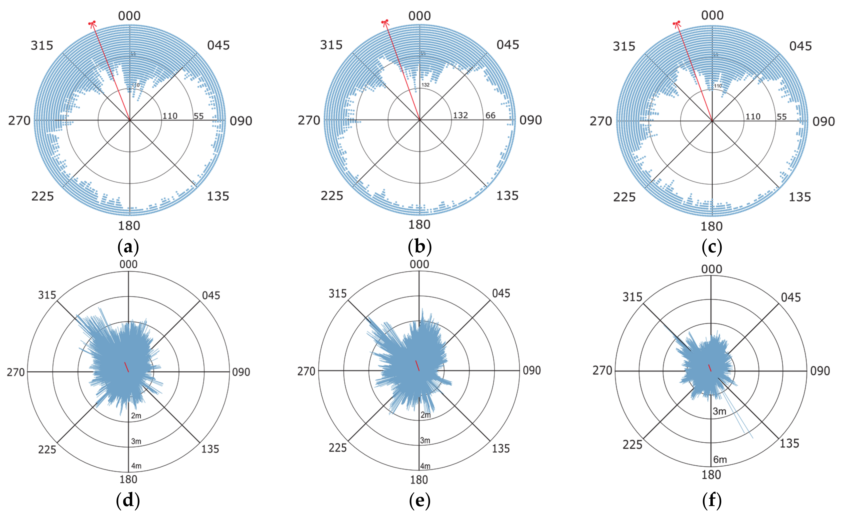
In this section, the circular analysis of azimuth distribution and the results of vector addition of azimuths and radius are presented. The results of circular statistics analysis are presented as follows. In Figure 13, stacked points on a circular histogram and deviation vector radius values are presented, and results in

Table 8. Circular statistics summary.

	Mean Azimuth	$\mathbf{Mean} \mathbf{Module} \left(\overline{\mathit{R}}\right)$	Circ. std. Deviation	Circular Variance	Circular Dispersal	$\mathbf{Von} \mathbf{Mises} \mathbf{Param}. \left(\mathit{\kappa }\right)$	Skewness	Kurtosis
GRAZ	338.8°	0.4	1.3°	0.6°	2.3°	1.0	0.2	0.2
PADO	340.5°	0.5	1.2°	0.5°	2.0°	1.0	0.2	0.3
MEDI	340.0°	0.4	1.3°	0.6°	2.4°	0.9	0.2	0.2

. The arrow line on histogram represents the mean deviation vector with corresponding 95% confidence intervals. Although the non-uniformity is evident, it is also characterized by mean module ($\overline{R}$) and von Mises concentration parameter (κ). Mean module represents the resultant of vector addition divided by the number of observations (or samples). Since the azimuths are considered as unit vectors, the module can be in range from 0–1, with larger values indicating directionality. The von Mises parameter represents a measure of data concentration in preferred direction. Value of 0 indicates uniform distribution, with non-uniformity taking place when the value increases.

The von Mises parameter value is considered significant when it is greater than 2 [42]. Furthermore, the hypothesis for angular uniformity was rejected using the Rao and Rayleigh uniformity tests. Therefore, non-uniformity and directionality for all stations can be observed.

In Figure 13a–c, respectively, in the first row are circular histograms with dots representing counts of azimuths in the observed direction. Likewise, the mean azimuth is depicted as a red arrow line with red dots representing limits of confidence intervals. Figure 13d–f, respectively, in the second row show the deviation vectors with visible red line representing the resultant vector.

The resultant deviation vector value is calculated by vector addition [12]. Azimuths are expressed in degrees, with radius values in meters. Resultant radius values are 0.43 m for Graz, 0.44 m for Padova, and 0.32 m for Medicina, compared to mean linear radius values at approximately 0.85 m. The mean azimuth of approximately 340° was observed for all stations, indicating displacement towards navigational quadrant IV (270° to 360°). The larger number of observations in navigational quadrants IV and I (000° to 090°) was evident.

It must be considered that the mean radius value, as presented in Table 6, is an arithmetic mean of all radius values calculated and converted from the Cartesian coordinates. This value is calculated when only the magnitude is considered. The radius value calculated from the resultant deviation vector addition considers both the magnitude and direction. Therefore, this is the resultant value from all vectors. Finally, the radius value which is calculated as a square root of means of squared latitude and longitude deviations must be mentioned. This is the DRMS value or quadratic mean. This was also noted in Reference [15] and should be considered when analyzing and interpreting mean radius values, as presented in Table 6 and respective presentations. The analyses show directionality for all stations, towards the same direction or more appropriate, the sector. This corresponds to the linear analysis in the Cartesian coordinate system and the respective density observations. The slight bimodality can be observed for navigational quadrants III (180° to 270°) and IV (270° to 360°).

4. Discussion

The error concentration was observed in two northern navigational quadrants for all reference stations, confirming the overall positional similarity. Further, circular statistics were required to describe directionality of positioning deviations direction and calculate deviation vector means. Furthermore, when considering radius values (magnitudes) in the polar coordinate system, careful interpretation of measures is required, when compared to linear values.

Considering latitude and longitude positioning deviations distribution, the results were as expected. There were no significant departures from normality and the radius magnitude can be approximated with Rayleigh or related distributions. Other distribution approximations must be considered in relation to variances, which are not equal for latitude and longitude deviations. This inequality can result from satellite geometry in higher latitudes [40] and from the other error budget contributions. As a matter beyond the scope of the research, the positioning error causes may be the subject of further work.

In Reference [15], the need for complementary circular and linear analysis was discussed in the context of the positional accuracy of satellite images geometric corrections. When considering the analysis of GPS positional accuracy, the need for such complementarity is not immediately obvious. However, comparable observations are valid, as in the beforementioned case. The error behavior between stations is similar, with slight departures in the common positioning patterns. The reasons can be found, among other things, in the common modeling approach, for example due to the tropospheric delay, given the differences in IGS stations heights. As for the similarities, they are observable with linear statistics, i.e., deviation density and the spread from a true position. Considering average radius magnitude values, it indicates that the expected position can be placed anywhere around the true position. The directionality of the random error segment of the total error is not relevant. However, the error components are also non-random, accounting for systematic error and its estimate, the bias. For that, vector resultants, directionality and circular averaging provide further insights. Moreover, the vectorial error comparison, alongside scalar (linear) accuracy measures are useful. They could be used as an indicator for positioning deviation behavior differences between larger number of regional stations or between regions themselves. Vectorial differences representing distortions, misalignments, and non-uniformity in planar satellite images could be interpreted similarly in the context of positioning. Therefore, the deviation vectors are viewed as a representation of two-dimensional horizontal error surface or the positional error field. This analogy can be extended in three dimensions. Expressing positional error value as a vector is more complex since a vector has direction and magnitude. However, it is also intuitive for interpretation, in terms of error displacement from the coordinate origin, or the relative reference frame. Positional error displacement is commonly expressed and interpreted in componential orthogonal coordinates and probability values. Nevertheless, the magnitude and directionality of errors are perceived and assigned, regardless of whether they are explicitly expressed or not.

In this baseline research, non-random error source components and their contribution to total positioning deviations have not been analyzed. However, certain positioning error causes can be addressed. The distribution of satellites providing positioning signals was not uniform at elaborated latitudes (approximately 45° N), and the resulting positioning deviation distributions relative to satellite geometry were expected to a degree. The reasons can also be found in receiver microenvironment (e.g., multipath and hardware thermal noise) and the discrepancies in estimated and real satellite ephemeris, as well as in both satellite and receiver delays in instrumental equipment. According to the geomagnetic activity, the geo-environment was considered as stable, however other, potentially influential space weather indicators were not analyzed. Unlike the receiver noise and multipath [43], some of the components are stable and predictable, such as satellite geometry, timing, and ephemeris, and atmospheric errors [8]. This must be considered in future systematic positioning deviations assessment. Furthermore, observations were not sampled randomly from all available observations in the 11-day observational period. The observed navigational quadrantal distribution and inequalities should be further examined in relation to total position deviation distribution and the consequent systematic error influence. With presented methodology and observed quadrantal inequalities, the Dilution of Position (DOP) can be assessed for individual quadrants, resulting in precise quadrantal distribution.

Since this analysis was based on propagation media modeled positioning solutions, the positioning deviation distributions may have been influenced by the models itself. Although it would have been interesting to employ a GPS receiver as a true sensor rather than the positioning mean, and therefore not contaminated with model effects, the unmodeled observables analyses remain one of the steps towards further research activities.

5. Conclusions

In the conducted research, satellite positioning accuracy and positioning deviation error distribution in the Adriatic region were evaluated using different statistical approaches. Linear statistics revealed that northern navigational quadrants (IV, I) had more deviated positions. Elliptical error spread was observed, as well. Quadrantal analysis was conducted as a subset of total positioning deviation distribution, due to observed error distribution navigational quadrants inequalities. Navigational quadrant analysis revealed that the positions are mostly situated in the quadrants IV and I, followed by navigational quadrants III and II. Mean quadrantal latitude and longitude deviation values are expressed relative to the respective navigational quadrant. Therefore, they are larger than the mean total value calculated for all navigational quadrants.

Statistically and observationally, positional deviations behavior in the Adriatic region during quiet space weather conditions period was similar. Latitude and longitude deviations were mostly normally distributed with very weak correlations. Therefore, the resulting positional two-dimensional distribution can be approximated with Rayleigh distribution. Based on the results, besides Rayleigh, radius distribution can be approximated with Weibull and gamma distribution, as well.

Circular statistics methodology complemented linear error analysis. Mean azimuth value was approximately 340° for the selected stations with evident non-uniformity. The resultant error radius values by vector addition are 0.43 m for IGS Graz, 0.44 m for IGS Padova, and 0.32 m for IGS Medicina. Furthermore, with vectorial deviation representation, mean magnitude and direction were observed. The usage of position deviation vectors can facilitate the assessment of position deviations displacement and isotropy considering individual and multiple stations.

Further research will address non-modeled observables. In that sense, GPS receiver would be analyzed as a sensor fully without model induced biases. Other observational periods and regions must be evaluated against the observed results. Positioning deviation analysis should concern error components, including satellite geometry and other influencing parameters, such as multipath and satellite and receiver differential code biases. The space weather activity has to be considered, as well, to evaluate the positioning distributions entirely and cover all influential segments.