
NagareDB: A Resource-Efficient Document-Oriented Time-Series Database
by
 ,
,
Carlos Garcia Calatrava
1,2,* ,
,
Yolanda Becerra Fontal
1,2,
Fernando M. Cucchietti
1 and
Carla Diví Cuesta
1 1
Barcelona Supercomputing Center, Plaça Eusebi Güell, 1–3, 08034 Barcelona, Spain
2
Department of Computer Architecture, Universitat Politècnica de Catalunya (BarcelonaTech), C. Jordi Girona, 31, 08034 Barcelona, Spain
*
Author to whom correspondence should be addressed.
Data 2021, 6(8), 91; https://0-doi-org.brum.beds.ac.uk/10.3390/data6080091
Submission received: 14 July 2021
/
Revised: 5 August 2021
/
Accepted: 6 August 2021
/
Published: 13 August 2021
(This article belongs to the Section Information Systems and Data Management)
Abstract
:The recent great technological advance has led to a broad proliferation of Monitoring Infrastructures, which typically keep track of specific assets along time, ranging from factory machinery, device location, or even people. Gathering this data has become crucial for a wide number of applications, like exploration dashboards or Machine Learning techniques, such as Anomaly Detection. Time-Series Databases, designed to handle these data, grew in popularity, becoming the fastest-growing database type from 2019. In consequence, keeping track and mastering those rapidly evolving technologies became increasingly difficult. This paper introduces the holistic design approach followed for building NagareDB, a Time-Series database built on top of MongoDB—the most popular NoSQL Database, typically discouraged in the Time-Series scenario. The goal of NagareDB is to ease the access to three of the essential resources needed to building time-dependent systems: Hardware, since it is able to work in commodity machines; Software, as it is built on top of an open-source solution; and Expert Personnel, as its foundation database is considered the most popular NoSQL DB, lowering its learning curve. Concretely, NagareDB is able to outperform MongoDB recommended implementation up to 4.7 times, when retrieving data, while also offering a stream-ingestion up to 35% faster than InfluxDB, the most popular Time-Series database. Moreover, by relaxing some requirements, NagareDB is able to reduce the disk space usage up to 40%.
1. Introduction
The great progress in the technological field has led to a dramatic increase in deployed monitoring devices. Those devices, commonly called sensors, are employed in a broad number of scenarios, ranging from traditional factories and commercial malls to the largest experiment on Earth [1].
The continuous polling of the sensor’s readings is considered beneficial, as it helps not only in supervising the status of the monitored assets, but also in understanding the behavior of the monitored systems by collecting insights [2]. Moreover, sensor data started being used in Data Analysis and Machine Learning approaches such as Industrial Predictive Maintenance, in order to anticipate to future failures, and Anomaly Detection, aimed at identifying rare events or observations.
In general, in order to optimize the value extracted from data, it is necessary to keep a large historical record. In consequence, Monitoring Infrastructures are expected to work closely with database management systems, whose goal is to efficiently store and manipulate data for its later retrieval.
While General-purpose database management systems (GDB), such as Relational Database Management Systems, have been historically capable of managing a wide range of scenarios, they were found inefficient, or even unsuitable, in handling the Velocity and Volume of nowadays’s large Infrastructures [3].
In order to address the specific challenges of Monitoring Infrastructures, specialized systems like Time Series Database Management Systems (TSBD) arose. TSBD are specially tailored to the nature of sensor readings, where each entry is associated with a timestamp, being able to efficiently represent them as a sequence of values over time.
As monitoring systems attracted more and more interest, along with the Internet of Things (IoT) boom, TSDB grew in popularity, becoming the fastest-growing database type from 2019 [4]. In not many years, altogether with the NoSQL movement, DBMS moved from one-size-fits-all, where one single technology was applied to every scenario, to a situation in which a single scenario, such as Time Series, could be implemented with a plethora of different technologies [3], each one with different performance, functioning, requirements, and even query language.
As a consequence, implementing capable solutions involving Time-Series databases became fairly laborious to small and medium-sized organizations [5] (SMEs), that wanted to benefit from Monitoring data, but lacked the resources needed to build those specialized data handling architectures, facing three different obstacles:
- Hardware: Handling real-time data requires computing resources in line with the Monitoring Infrastructure’s size. Moreover, as time passes and more data is gathered, the storage requirements grow accordingly. A common approach to tackle this problem is to just keep a fixed amount of data, following FIFO method: As new data is stored, the oldest is removed. This is therefore a double-sided sword, since it prevents storage costs to grow, but it also implies that data is being discarded, and potentially relevant information is lost.
- Software: While some databases are open-source, most popular databases offer both a limited-free version and a commercial-enterprise edition. However, license pricing is only one of the many considerations to take into account: for example, large-scale Monitoring Infrastructures typically require the software to be horizontally-scalable, so, able to scale out by adding more machines.
- Expert Personnel: Following Monitoring Infrastructure’s rising interest, TSDB became the fastest-growing database category, leading to a plethora of new databases. Furthermore, each database typically has a different query language and a completely different way-of-thinking associated with its usage. However, Data Engineers are expected to select and master the most appropriate solution for each situation. Consequently, experts are not easy to find or train, nor cheap to hire [6].
The main contributions of this paper is towards relieving the above explained problems, helping in the democratization of Monitoring Infrastructures, by lowering down the barriers to employing a Time-Series Database. Concretely, we demonstrate and benchmark the novel approach followed for implementing NagareDB, a resource-efficient Time-Series database built on top of MongoDB—a database typically discouraged in the Time-Series scenario [7,8,9].
NagareDB intends to ease access to the essential resources needed by: First, by working on top on a open-source and broadly-known database such as MongoDB, which relieves SMEs from licensing costs, and personnel from learning to use from scratch yet-another database. Secondly, by offering a fair trade-off between efficiency and requirements, which makes it able to be deployed in commodity machines while offering outstanding performance.
More precisely, our experiments show that NagareDB is able to outperform MongoDB’s time series data model, providing up to a 4.7 speedup when querying, while also offering a 35% faster synchronous real-time ingestion, in comparison with InfluxDB, the most popular Time Series Database, whose non-scalable version is open source.
Moreover, thanks to the optional usage of a naive-but-efficient data type approximation, NagareDB is able to provide further querying speedup while reducing the disk space consumption up to 40%, which makes it able to store an almost 1.7 times bigger historical period in the same disk space.
2. Background
2.1. Solutions Categorization
Concerning Time-series data management, Databases can be efficiently-implemented following a wide range of data models such as key-value or column oriented data models [10]. However, this research focuses on their outcomes and purpose, in disregard of their internal implementation. Consequently, Time-series databases could be classified either in General-Purpose DB, or Purpose-Built Time-Series DB, which, in turn, could be considered either Native TSDB or Adapted TSDB.
General-purpose databases (GDB). GDB intend to meet the needs of as many applications as possible. In consequence, GDB are designed to be independent with regard to the nature of the data to be handled. Thanks to this Swiss army knife behavior, GDB are typically the most popular DBMS, which makes it easier to find expert personnel in their usage [4]. However, this flexibility is gained at the expense of efficiency, since GDB are not tailored to benefit from the specifics of any particular scenario [11]. Hence, system performance is limited, and strongly attached to the design decisions made by the database engineers, while fitting the particular scenario into the GDB.
Native Time-Series databases (N-TSDB). N-TSDB are DBMS that are optimized for storing and retrieving time series data, such as the one produced by sensors or smart meters. As TSDB are tailored to the specific requirements of Time series data, they can be offered as an out-of-the-box solution, meaning that not many design decisions have to be taken, speeding up the deployment time. However, as a consequence of their intrinsic specialization, their popularity is substantially reduced, in comparison to General-purpose DBMS [4].
Adapted Time-Series databases (A-TSDB). This specific case of TSDB does not employ a new database engine, but borrows one from a GDB. Specific functionalities and design decisions, with respect to the time series nature, have been implemented on top of a GDB, offering the outcome as an out-of-the-box solution. Thus, the newly created database looses the ability of handling scenarios that was typically able to. As the foundation data model is inherited from the GDB, the optimization approaches than can be performed are limited. Thus, A-TSDB rely on the popularity and robustness of the chosen GDB, while providing an scenario-optimized solution.
2.2. Time-Series Properties
Time-Series DBs are tailored to the specifics of Time-Series data, which empowers their efficient data handling. Some of the most fundamental properties of time-series data [12,13] are:
- Triple-based Data Model. Time series data is mainly composed of three parts: The subject to be measured (f.i sensor ID), the measurement, and the timestamp at which the measurement was read.
- Smooth and continuous stream. The writing of time series data is relatively stable, and its generation is typically done at a fixed time frequency.
- Immutable data. Once data is read and written, it is never updated, except in case of manual revisions.
- Decaying query probability. Recent data is more likely to be queried. Thus, as newer data is ingested, the older data has less chances of being consulted.
2.3. TSDBs Requirements
Time-series databases can be implemented following a wide range of approaches in order to benefit one or another feature or specific use case requirements. For example, a given TSBD could be designed in order to maximize the ingestion speed, while other might intend to speed up data retrieval.
While optimizing at the same time some of these requirements might be possible, sometimes it is necessary to find a trade-off [14,15,16]. In addition, some non-functional requirements might depend on the target users or even the business model of the database developers.
This research classifies TSBD requirements according to the resource that benefit or compromise the most, as explained in Section 1. Concretely:
- Software. Requirements regarding software characteristics or database functionalities, involving query or data types, allowed operations, etc.
- Hardware. The ones regarding the ability of the database to reduce or to optimize the machine(s) speed or resources usage.
- Expert personnel. These requirements describe the different ways the user is able to interact with the database, including the facility of its usage or the compatibility of the database with the user’s environment.
- Software.
- –
- Continous calculations. The TSDB is able to resolve functions continuously, taking into account the recently ingested data, and the historical information, keeping the outcomes internally. An example is the continuous calculation of the last hour average value, for a given item.
- –
- Time Granularity. It defines the smallest time unit precision in which a timestamp can be stored and interpreted. For example, a given TSDB could be able to store up to seconds, being unable to keep information regarding the millisecond in which the data was generated.
- –
- Aggregation. When aggregating, the database is able to group multiples values and perform operations over them, returning a single result. The retrieval of the minimum/maximum value during a given time period is an example of aggregation.
- –
- Downsampling. It is the process of reducing the sampling rate of a given data source or sensor, taking into account a specific time granularity or sample interval. For example, if the database stored a sensor reading in minute-basis, the database should be able to retrieve its data in hourly intervals, showing, for example, the average of the total sensor readings for each hour.
- –
- License. A license regulates, among others, who and how the database can be used. Since this research focus on being resource-efficient, the price or cost of licenses, for using a given database, is especially relevant.
- Hardware.
- –
- Distribution/Clusterability. Scalability and load balancing features are able to compensate machine failures, preventing the system from down-times. Moreover, by scaling horizontally, the database is able to increase its storage or its performance, by adding further nodes or machines to the cluster.
- –
- Retention Policy. In a TSDB, a data Retention Policy specifies for how long data should be kept in the system, until being deleted. The possibility of setting up retention policies is crucial for TSDB, as keeping the data forever is not typically affordable for most users, as hardware storage might be limited and expensive.
- –
- Storage Approach and Compression Algorithms. The approach followed for implementing the data persistence will directly affect the storage usage of the database and its compression capability. For example, databases implemented following column-oriented data models are likely able to compress data more efficiently, by means of Run Length Encoding [17]. Moreover, each database employs a given compression algorithm, reducing either its disk usage, its compression time or finding a trade-off [18].
- –
- Ability to support highly concurrent writes. Data is typically ingested at a regular pace, following the Smooth and continuous stream property explained in Section 2.2. However, it is important for the database to be able to ingest it as fast as possible, as it enables a wider range of scenarios, including more demanding ones.
- –
- Ability to retrieve data speedily. Queries should be answered as fast as possible, as the TSDB might be the cornerstone of further systems or operations, such as data exploration or visualization, data analysis, or machine learning techniques such as predictive maintenance or anomaly detection [19,20].
- Expert personnel.
- –
- Database and Query Language Popularity. As a database raises more interest, it becomes easier to find expert personnel on its usage, clear documentation and even courses or training material. The same effect happens with the query language: While some databases use their own language, some others mimic, inherit or support a more popular and external query language, in order to facilitate its querying.
- –
- Interfaces. Interfaces can be used by programming languages to communicate to a database. Thus, the more interfaces a database provides, the easier it becomes to adapt to personnel expertise.
- –
- Operative Systems. As it happens with interfaces and query languages, users might be specialized in a given operative system. Moreover, some companies could promote the usage of a given operative system. Thus, as more Operative Systems the database is able to be deployed in, the more possibilities it will have to fit in its user’s environment.
3. Related Work
The problem of handling time-series data has been addressed by employing or developing different database solutions laying in one of the three categories explained in Section 2.1. Concretely, just DB-ENGINES, the Knowledge Base of Relational and NoSQL Database Management Systems [4], keeps track of more than 35 Time Series Databases, such as InfluxDB, KdB+, Prometheus, Graphite, or TimescaleDB. While their shared goal is to empower data management, their approaches, strengths and weaknesses are different, being InfluxDB the most popular Native Time-Series, and TimescaleDB the most popular Adapted Time-Series database [4]. Thus, some of the most relevant technologies related to this research are:
MongoDB. It is a general-purpose open-source database written in C++ [21]. It offers an extremely flexible data model, since its base structure is document-oriented, so, made out of JSON-like documents. These documents act like independent dictionaries where the user can freely add of remove new fields, releasing the database of up-front constraints. Thus, there is no need to set up or alter any enforced global schema, as it would happen in relational databases [22,23]. However, this flexibility implies constant metadata repetition, such as the key of the key-value JSON dictionary pairs. This negative impact is partially palliated by its data compression mechanisms [24]. It is able to scale horizontally freely, by means of shards and replicas, which makes it possible to create a database cluster composed by commodity machines. Regarding its interaction methods, it has its own query language and a really wide range of interfaces to work with. It is able to perform continuous queries when retrieving new values by means of change streams and to aggregate and down-sample data. Last, it can be installed on Linux-based systems, OS X, and Windows, which makes it able to reach a great number of users. However, although it is considered the most popular NoSQL DBMS [4,25], its usage in the Time-Series domain has been typically discouraged due to its time-expensive query answering [7,8,9], and its timestamps are limited to milliseconds [26], which might be insufficient for high-demanding use cases. Last, although it provides optional retention policies, in the form of capped collections, they are tight to the insertion date of a given sensor reading, and not to its generation date [26], which might be problematic for some time-series use cases, in case of delays or non-chronological insertions.
InfluxDB. It is a native Purpose-Built Time-Series database [27] written in GO. From 2016, it is considered the most popular TSDB [4]. It supports plenty of programming languages and two different querying approaches: Flux, its own query language, and InfluxQL, as SQL-like support, each having different limitations. It is able to efficiently perform a wide range of operations, such as continuous querying, down-sampling and aggregations. Moreover, is able to efficiency reduce and limit disk usage, by means of its compression mechanisms and its data retention policy. However, it provides a commercial enterprise version and an open-source version, with some limitations. Among others, the open-source version is not able to grow horizontally, so the deployment is limited to one single machine [27], not being able to carry out data sharding or replication, which strongly limits the performance, at the same time that reduces the system availability and fault-tolerance. Regarding its potential user’s operative systems, it can be installed on Linux-based systems and OS X, but not on Windows itself. Last, although it is the most popular TSDB, its popularity score is almost twenty times smaller than other general-purpose databases, such as MongoDB [4].
TimescaleDB. It is an adapted open-source TSDB built over PostgreSQL, one of the most popular General-Purpose DBMS [4]. Thus, it inherits PostgreSQL’s broadly known SQL query language and its powerful querying features and interfaces, which lowers down its learning curve. Moreover, it is able to run on Windows, OS X, and Linux, which makes it able to reach a wide number of potential users. However, due to the limitations of the underlying rigid Relational data model, its scalability might be compromised, and its performance might vary depending on the query [28]. Moreover, as its underlying data model is row-oriented, its disk-usage consumption is significantly greater than other TSDB, such as InfluxDB [28], and its compression mechanisms are not likely able to demonstrate its full potential [29].
To sum up, on the one hand, MongoDB is a general-purpose and open source database, but despite being considered the most popular NoSQL DBMS, its usage in the time-series scenario has been discouraged. On the other hand, TimescaleDB relies on a well-known SQL solution and offers good optimizations, but generally worse than Native TSDBs. Last, InfluxDB offers an upstanding performance, but its usage is limited to Linux-based and OS X, at the same time that its full version is commercial-licensed, which reduces the number of users that could benefit from it. In addition, as it is a native TSDB, it becomes necessary to learn a new technology from scratch.
NagareDB’s goal is to provide a fair trade-off between efficiency and resources demand, offering an optimized TSDB solution that relies on a moldable, open-source, and well-known NoSQL General-purpose DBMS.
4. Design Approach
This section describes the holistic and most relevant design decisions materialized in NagareDB, with the goal of creating an efficient and balanced Adapted Time-series database. In addition, it states the main differences between the MongoDB Recommended Implementation [30] for Time-Series (briefed as MongoDB-RI), and other related solutions.
4.1. Data Model
As in any adapted database, the overlying data model adaptability is limited by the malleability of the foundation data model. Taking this into account, our Time-Series Data Model approach has the following key features:
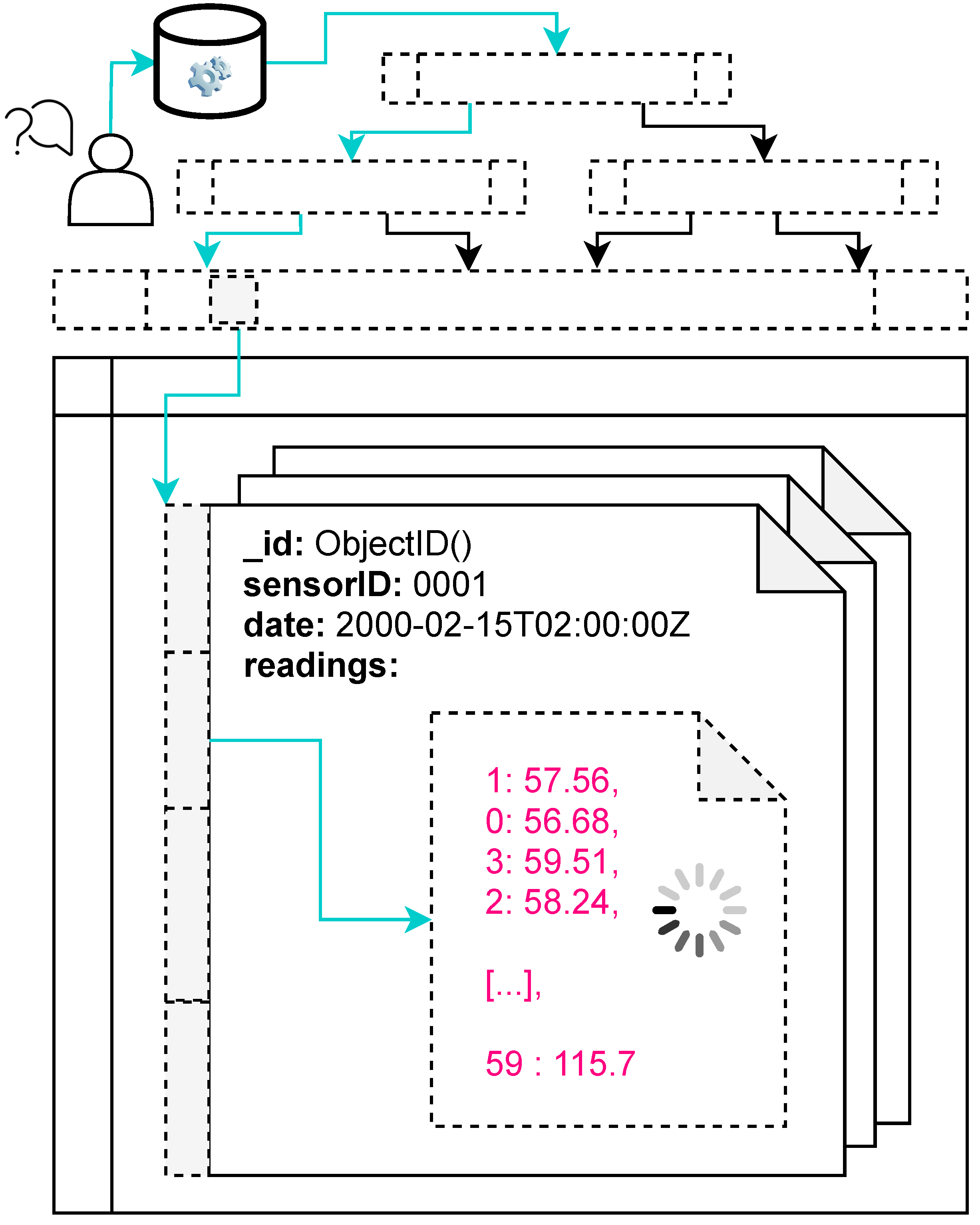
Medium-sized time-shaped bucketing. Sensor readings are packed together in medium-sized buckets or documents, following the nature of time. Concretely, a document clusters together the readings of three consecutive units of time. For instance, if the frequency unit in which a sensor is reading values is set to minute (First unit), all readings belonging to the same hour (Second unit) will be packed together, for afterwards being bucketed in a daily document (Third unit). This structure can be seen in Figure 1: The showed document represents the 15th day of Month 02/2000 (3rd time unit), that stacks together all 24 day hours (2nd time unit), were each hour has 60 readings, one per minute (1st/base time unit). By contrast, MongoDB-RI packs together readings in small-sized buckets, taking just 2 time units. This can be seen in Figure 2, were a document represents an just hour and its minutely readings. While this could be efficient for short-ranged queries, it severely penalizes medium and high ranged historical queries, as the storage device is asked to retrieve a large amount of documents, that could be scattered. Since long queries are more resource-consuming than small ones, this approach is considered more balanced.
Time rigidity. Following the smoothness property explained in Section 2.2, sensor readings are organized via a rigid schema-full approximation, meaning that there is a pre-defined rigid structure for their storage, where each reading has an specific allocation and position. This bucket structure, consisting in a dictionary of arrays, is created as a whole when a sensor reading, belonging to it, is received. This structure can be seen in Figure 1, where the document representing the 15th day of 02/2000 has several pre-defined and fixed-size data structures. As one of the most important features in MongoDB is its schema-less design, enforcing a schema could be seen as counter-intuitive at first sight, however, imposing a structure provides two important benefits, perfectly suited for time-dependent data: First, it allows to store time-sorted data in disk, and second, it allows to leverage from implicit information, inherent to the structure design, such as the value array position. Conversely, MongoDB recommended data model (Figure 2) following its schema-less nature, keeps sensor readings dictionaries, where the key provides recurrent explicit information about time (f.i the minute when the reading was performed), and the value contains the sensor reading itself.
Sensor elasticity. With respect to the sensor dimension, it follows the schema-less approximation inherent to MongoDB. Consequently, new sensors can be incorporated or removed in an elastic way, without having to alter any global schema, as it could happen in rigid data models such as relational ones [22,23].
Pre-existing timestamps. Every sensor reading is implicitly assigned to an already existing timestamp. Thus, timestamps are not calculated on the fly, as it happens in MongoDB-RI.
Data-driven bucket identification. Each bucket is identified and sorted by sensor’s reading time. By contrast, MongoDB-RI identifies and sorts buckets by metadata, such as insertion time. However, in Time-series scenarios, sorting by insertion time is not necessarily equal to sorting by data-generation time, as data could be delayed or even ingested disorderly.
4.2. Access Structures and Layered Bucketing
Sensor readings, containerized in buckets as explained in Section 4.1 and in Figure 1, are hash-distributed and grouped, according to time, in so-called MongoDB collections. More precisely, a MongoDB collection, containing a set of documents sorted by a B-Tree, is intended to keep the data produced in a given month, and in a specific year. For example, as it can be seen in Figure 1, the bucket containing the readings of sensor 0001 for the day 15 February 2020 is classified in the collection Month 2000_02.
This bucketing approach intrinsically enables, on the one hand, the possibility of performing efficient lazy-querying, eventually performing several small queries (one per bucket) instead of a big one (whole database query). Moreover, querying can performed by means of chained queries, so, performing several time-consecutive queries, relieving the system from searching or holding data that is not yet needed. On the other hand, when querying speed is crucial, this bucketing approach also enables efficient parallel querying, as data is already naturally grouped, being able to perform several queries to different buckets at the same time. Last, benefiting from both the decaying and immutability properties of Time-series (Section 2.2), this bucketing approach allows the natural compaction of already filled-up buckets, that are not likely to be updated, which also have less possibilities of being queried.
Using a more granular bucket distribution, such as grouping data by its generation day, instead of its generation month, while tempting for high-granularity data, is currently discarded in this approach, but subject to future re-considerations. This is due to the fact that MongoDB’s WiredTiger Storage Engine requires the Operative System to open two files per collection, plus one per each additional index [26], which could overwhelm the Operative System’s open files table. This is, actually, a recurrent problem found in InfluxDB [31], which makes it necessary for database administrators to apply patches, for example with the ulimit command [32]. However, as NagareDB is intended to be a fast-deploying and resource-compromised solution, this self-imposed limitation was preferred.
By contrast, MongoDB-RI’s strategy is to keep data stored as a whole, accessing it via a single B-tree. However, this B-tree is intended to be kept in RAM [26], independently from the time range of the query to be performed. While this benefits efficiency, it potentially misallocates RAM resources. Conversely, the approach proposed in this research intends to save resources, by selectively loading and replacing small indexes based on the time-range of the queries, following a Least Recently Used approach.
4.3. Retention Policies
Retention policies are crucial in Time-Series databases, as the amount of data to be kept is limited by the available resources. Concretely, retention policies describe for how long a record needs to be stored in the system.
In order to tackle this problem, NagareDB proposes a flexible retention policy strategy, with the aim of finding a good trade-off between resource-saving and efficiency.
Concretely, the flexible retention policy is configured with a maximum and a minimum retention time. Thus, data will be eventually bulk-deleted in some point in between the minimum and the maximum allowed time.
The main advantage of this strategy is its instant and inexpensive bucket delete operations. For instance, if the retention time is set in terms of months (so, the number of buckets), the oldest data could be deleted as a whole, by dropping the monthly bucket.
By contrast, in fixed retention policy strategies, such as the ones of MongoDB-RI [26] or InfluxDB [33], when a new record is received, the oldest one is removed, meaning that each insert operation is potentially triggering an implicit delete operation, which reduces insert performance, at the same time that overloads the system.
Moreover, MongoDB’s retention policy is based capped collections, and takes into account the last inserted record. However in Time-series scenarios, insertion time order is not necessarily equal to data-generation order, as data could be received disorderly.
4.4. Data Types
MongoDB has a wide number of available data types [26], which can be inherited to any specific-purpose database built on top. Concretely, but not exclusively:
- Array
- Date: Milliseconds since the Unix epoch (1 January 1970)
- Decimal128: High-precision decimal.
- Document
- Double: 64-bit signed floating point.
- Int32/64: 32-bit or 64-bit signed integer.
- String
In spite of the wide variety of data types provided by MongoDB, decimal values are always requesting, at least, 64 bits for storage. While the usage of 64-bit double-precision decimals might be required for some high-precision scenario, more modest and resource-limited scenarios might find a more balanced solution by limiting the number of decimals digits, using a 32-bit data type for its representation.
Furthermore, this would allow users to store the same historical period of data using, theoretically, up to half of the disk storage resources or, said in another way, to keep up to two times more historical data in the same disk space.
As 32-bit decimals are not implemented in MongoDB, and taking into account that one of the main goals of this research is to provide a resource-balanced solution, the proposed approach includes one further, optional, and naive data type, understood as a on-query-time limited decimal. This naive data type relies on two different data types:
- 32-bit signed Integer: It keeps the decimal number without the decimal point. Thus, the integer part and the fractional part of the number are stored together, without separation.
- BSON Document: It is a meta-data configuration document, functioning as a dictionary, that keeps, per each sensor, which is the desired maximum number of decimal digits. Also, it keeps a default setting, that will be used if no specific configuration is set, for a given sensor.
This naive-but-effective approach is intended to enable the storage of decimal numbers in 32 bits, while limiting the foreseen overhead produced by the type casting. Data rounding is automatically done at insertion time, and the consequent type casting is accordingly performed during ingestion and query time.
Taking into account that a 32-bit signed Integer is able to represent a maximum value of and a minimum value of , this on-query-time limited decimal is able to represent, for example, a maximum number of , when using four decimals, given that the number of decimal digits has to be static, and each decimal digit should be able to range from 0 to 9.
This self-imposed limitation is optional, and targeted to sensors with low or medium magnitude order variability. Concretely, its target scenarios are the ones in which Monitoring Infrastructures set up a retention policy, as explained in Section 4.3. For example, for resource-limited scenarios involving anomaly detection or predictive maintenance, in which real anomalies or failures rarely occur, it will likely be more relevant to keep more historical data, if the sensor data fits in this naive decimal data type, than keeping more decimal digits [34,35].
Regarding InfluxDB, its available data types are [33]:
- 64-bit floating-point numbers
- 64-bit integers: Signed and unsigned
- Plain text string
- Boolean
- Unix timestamp
Which makes it mandatory to use 64 bits for any kind of number.
4.5. Further Considerations
4.5.1. Horizontal Scalability
It is inherited from MongoDB, providing it via shards and/or replicas. By constrast, InfluxDB is only able to grow horizontally in its commercial version.
4.5.2. Compression
MongoDB uses snappy compression [36] by default, which intends to minimize the compression time. However, NagareDB is set up to use Zstandard compression. ZSTD is able to offer higher compression rates, while slightly reducing query performance [37]. However, as one of the main objectives of the proposed approach is to reduce resource requirements, this option is preferred.
4.5.3. Timestamps
MongoDB’s date type is limited to milliseconds. Thus, NagareDB is also limited to it. While it would be possible to create a new data type for storing nanoseconds, we consider it enough to keep up to milliseconds, as NagareDB is intended to provide a good trade-off between resources and features offer, not specifically targeting the highest demanding use cases. Conversely, InfluxDB uses nanosecond precision. This makes InfluxDB a more time-precise database, but it also implies that in a not-that-precise scenario it will keep unnecessary date information [38].
4.5.4. Query Parallelization
The bucketing technique explained in Section 4.2 enables intrinsic query parallelization, as data is already equally distributed in buckets. However, as NagareDB is intended to provide a good resource-outcomes compromise, query parallelization is only enabled for queries whose nature is CPU-DISK balanced, and limited to half of the available threads. For instance, queries that request a historical period will not use query parallelization, as their CPU usage is low. Conversely, queries involving data aggregation, which requires higher CPU usage, are parallelized.
4.5.5. Time-Series Granularity and Frequency
NagareDB is intended for discrete time series, with stable frequency and round timestamps, following the smooth property explained in Section 2.2. For instance, users are expected to define the baseline granularity for each sensor, and/or a default one. Thus, when receiving a reading, the timestamp will be truncated to the desired granularity. By contrast, InfluxDB does allow non-truncated timestamps, but strongly recommends to truncate them, as otherwise efficiency drops significantly [39]. This self-imposed limitation provides extended performance, at the same time that prevents users from inefficient practices.
5. Experimental Setup
The experimental setup is intended to enable the evaluation of the performance of NagareDB in moderate-demand use cases, as well as the effects of implementing more lightweight data types, such as the one explained in Section 4.4.
Concretely, the experimental set up is made against two different solutions: First, the MongoDB recommended implementation (MongoDB-RI), as a reference point. Second, InfluxDB, as it is considered the most popular Time-Series Database [4].
5.1. Virtual Machine
The experiment is conducted in a Virtual Machine (VM) that emulates a commodity PC, in accordance to NagareDB’s goals, as explained in Section 1.
More precisely, the VM is configured as follows:
- OS Ubuntu 16.04.7 LTS (Xenial Xerus)
- 4 threads @ 2.2 Ghz (Intel® Xeon® Silver 4114)
- 8 GB RAM DDR4 2666 MHz (Samsung)
- 300 GB-fixed size (Samsung 860 EVO SSD)
5.2. Comparative Software
- MongoDB 4.4 CE: Time-series Recommended Implementation, referred as MongoDB-RI.
- InfluxDB OSS 2.0: Referred as InfluxDB.
- NagareDB-64b: When globally using MongoDB’s 64-bit decimal data type.
- NagareDB-32b: When using the limited-precision data type explained in Section 4.4, set up to keep 4 decimals.
5.3. Data Set
In order to generate synthetic Time-series, we simulate a Monitoring Infrastructure based on the industrial settings of some external collaborators of our institution. Concretely, it is composed of 500 sensors, equally segmented in five different monitoring areas. Each sensor is globally identified by a number between 1 and 500, and ships data every minute.
Sensors readings (R) follow the trend of a Normal Distribution with mean and standard deviation :
where each sensor’s and are uniformly distributed.
The simulation is ran until obtaining a 10-years historical period, from year 2000 until year 2009, included, so no retention policy is set. In consequence, the total amount of triples is 2,628,000,000.
Other configurations, such as ones including a bigger number of sensors, are likely to provide similar results. This is due to the fact that seek times, in SSD devices, are typically a constant latency [40,41], in contrast with HDD devices. This effect makes HDD devices to be discouraged for database applications, to the extend that not even InfluxData has tested InfluxDB on them [42].
6. Evaluation and Benchmarking
This section demonstrates the performance of NagareDB in comparison to other database solutions, as explained in Section 5.
Concretely, the evaluation and benchmarking is done in three different aspects: Storage Usage, Data Retrieval Speed, and Data Ingestion Speed. Thanks to this complete evaluation, it is possible to analyze the performance of the different solutions during the persistent data life-cycle, with regard to the database scope: From being ingested, to being stored and, lately, retrieved.
6.1. Storage Usage
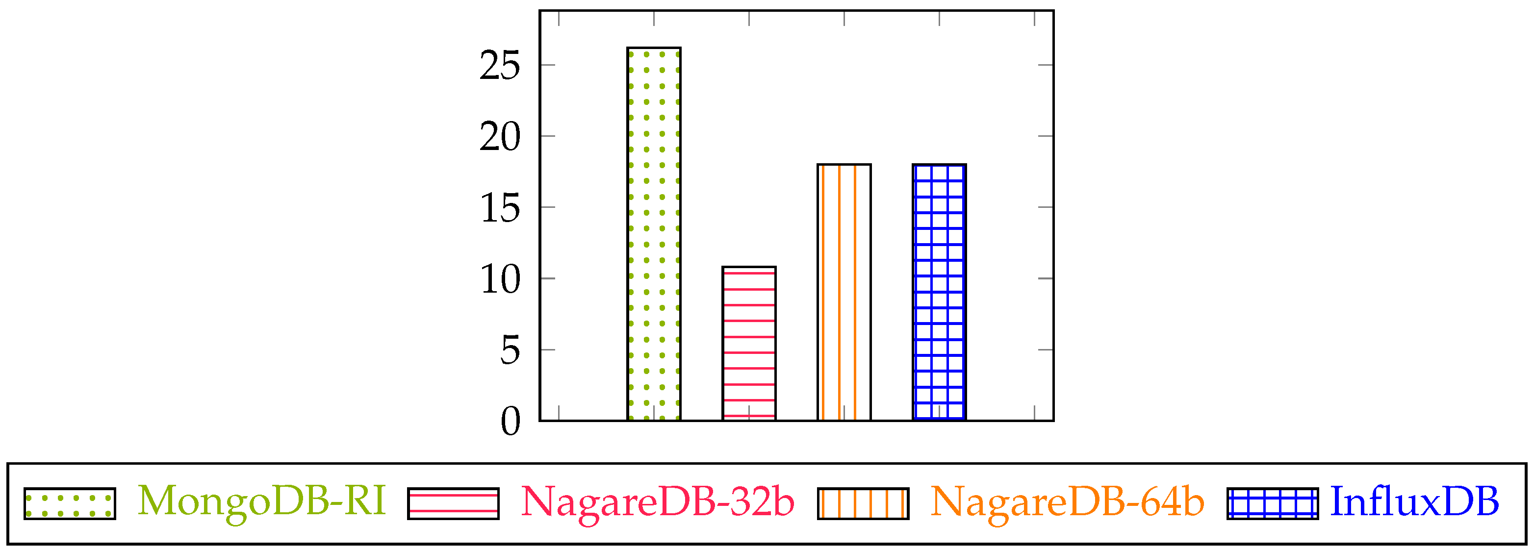
After ingesting the data, as explained in Section 5.3, the disk space usage of the different database solutions is as shown in Figure 3.
On the one hand, MongoDB-RI is the implementation that requires more disk space. This could be explained due its schema-less implementation and by its snappy [36] compression mechanisms intended to improve query performance while reducing its compression ratio, following the implications explained in Section 4.5.2.
On the other hand, both InfluxDB and NagareDB-64b require the same amount of disk space, which could be explained by its shared pseudo-column oriented data representation and by its powerful compression mechanisms.
Last, NagareDB-32b is able to reduce the disk usage by 40%, in comparison to both InfluxDB and NagareDB-64b, thanks to its lightweight data type, explained in Section 4.4. In consequence, NagareDB-32b is able to store, approximately, a 1.7 times bigger historical period in the same disk space.
6.2. Data Retrieval
The testing query set is composed by 12 queries (Table 1), intended to cover a wide range of use-case scenarios, while providing insights of the databases’ performance and behavior. They lay in four different categories:
- Historical querying: Obtain sensor readings for a specific time range. Answered with a dataframe. [Q1–Q7]
- Timestamped querying: Obtain sensor readings for a specific time instant. Answered with a dictionary. [Q8]
- Aggregation querying: Derives group data by analyzing a set on individual data entries. It is divided in two sub-categories:
- –
- AVG Downsampling: Reduce the granularity of the data by performing averages of individual readings. Answered with a dataframe. [Q9–Q10]
- –
- Single Value Aggregation: Obtains a single value from a set of individual readings, such as the Minimum value. Answered with a triplet (SensorID-Timestamp-Value). [Q11]
- Inverted querying: Ask for moments in time that matches certain value condition, instead of values in a specific instant. Answered with a dataframe. [Q12]
Each query is executed 10 times, one per each year (2000…2009), and we record the average execution time. The querying is always performed using Python Drivers. In order to ensure the fairness of the results, the cache is cleaned and the databases rebooted after the evaluation of each query.
6.2.1. Historical Querying
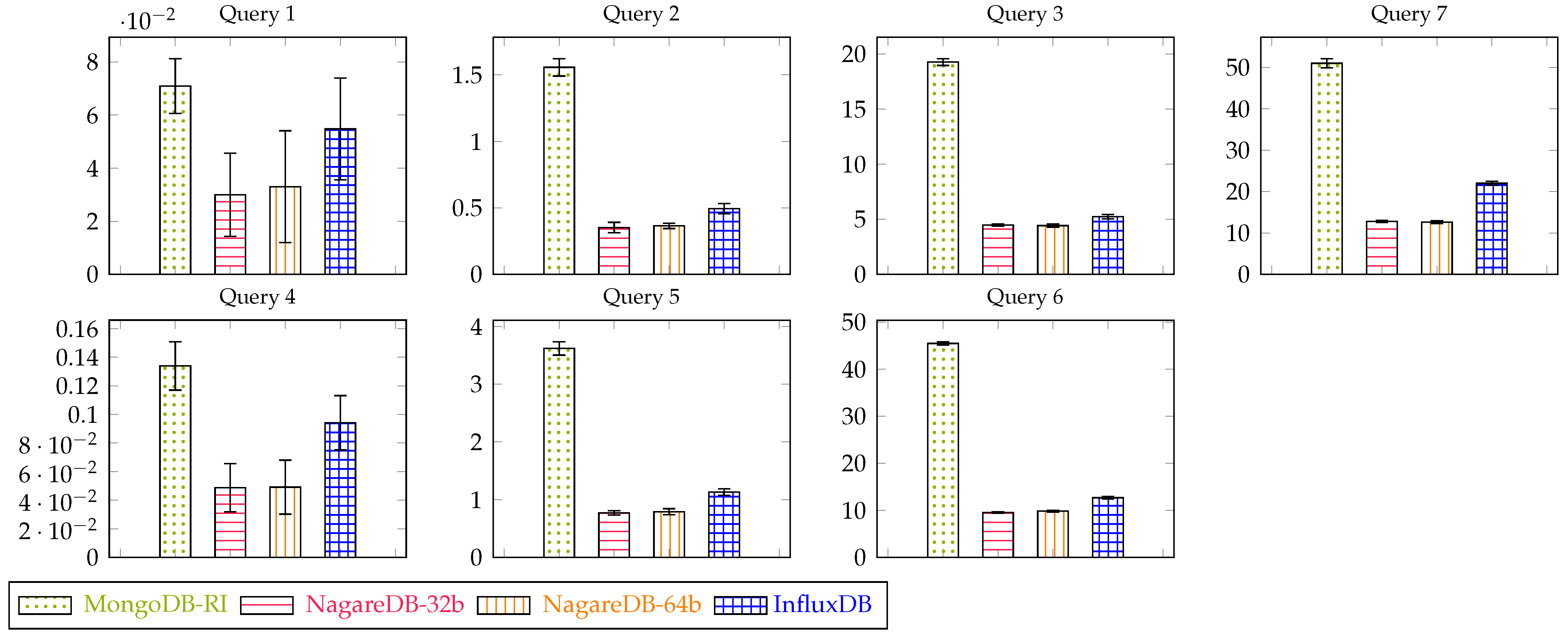
As it can be seen in Figure 4, NagareDB is able to retrieve historical data up to 5 times faster than MongoDB-RI, while also outperforming InfluxDB in every historical query. In addition, the plotting shows some interesting insights:
- MongoDB is faster when retrieving small historical ranges in comparison to when retrieving big ones. Concretely, NagareDB speeds up MongoDB by 2.5 in daily queries (Q1, Q4), while doubling the speedup when requesting a larger historical period. In contrast, InfluxDB performs better when retrieving more historical data.
- NagareDB-32b is generally faster than NagareDB-64b, but the difference is almost negligible in this category. This is due to the fact that, while it handles smaller data, it also performs internal type castings, as explained in Section 4.4.
- NagareDB slightly reduces its performance when retrieving sparse data (Q7). This effect also occurs in InfluxDB, but more notoriously.
6.2.2. Timestamped Querying
Timestamped querying requests all sensor values for a given timestamp. Hence, it does not benefit from the columnar design that NagareDB and InfluxDB follow, being penalized [29]. Thus, MongoDB, based on small buckets, is able to outperform them.
However, as it can bee seen in Figure 5, NagareDB is able to outperform InfluxDB using any of its data types. Moreover, NagareDB-32b is able to provide much better performance than NagareDB-64b. This is due to the fact that the data buckets, that have to be loaded to RAM, are much smaller, with the advantage that there is only one value requested per bucket, so the data type parsing overhead is greatly reduced.
Finally, it is important to take into account that this kind of query is answered fast, even in the case of InfluxDB, which shows the worst speedup. Concretely, NagareDB-32 only needs 0.065 seconds in order to answer the query. Thus, despite of the fact that MongoDB outperforms all three alternatives, the response times are still far acceptable.
6.2.3. Aggregation Querying
Both NagareDB and InfluxDB greatly surpass MongoDB-RI. This behavior is even more notable in downsampling queries (Q9–10), as seen in Figure 6. More precisely:
- InfluxDB is more efficient when performing queries that involve big amounts of data, but the outcome is calculated by reducing it, such as downsampling queries. However, when the result consists in one single value, such as minimum-value detection queries (Q11), NagareDB is able to outperform it.
- NagareDB-32b outperforms NagareDB-64b as NagareDB-32b is able to read values slightly faster, without the negative impact of performing numerous type castings.
Concretely, unlike when querying historical data, NagareDB-32b needs to process all the data, but it is only request to perform one type casting per every 60 sensor readings (R) (on the average result, in this case), as the base granularity is minute, but the target granularity is hour:
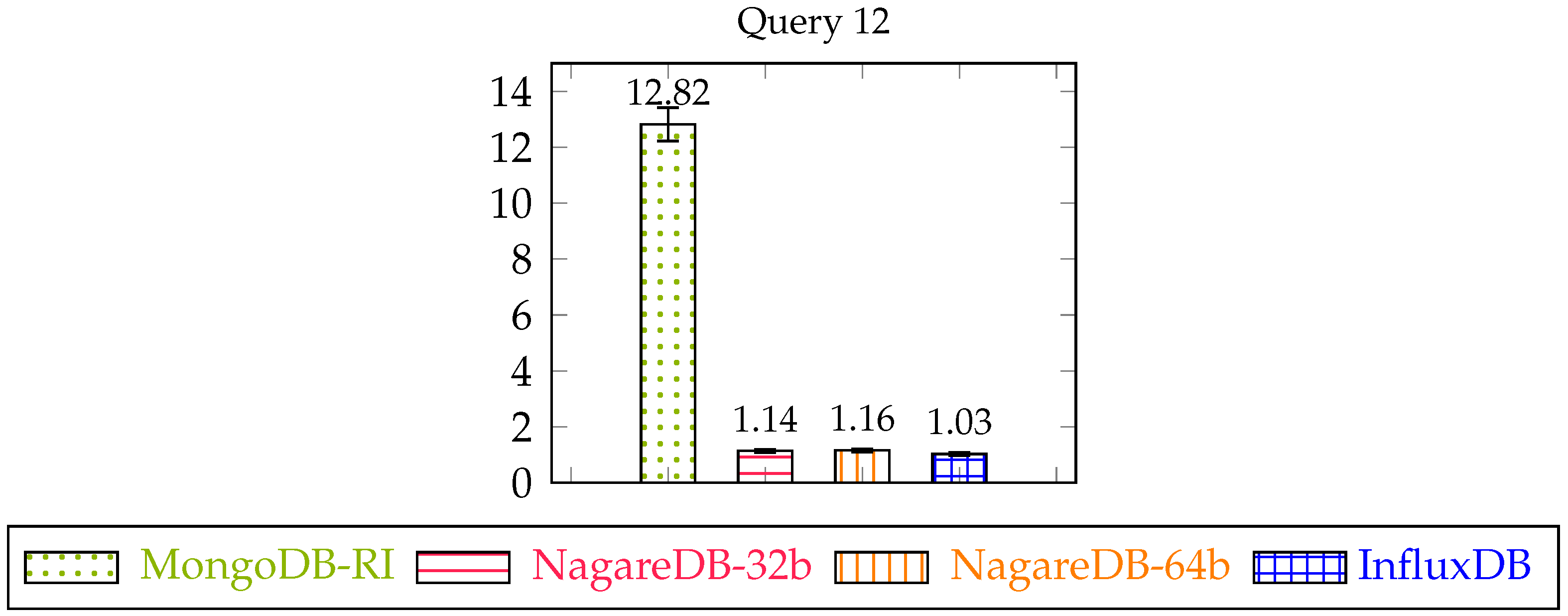
6.2.4. Inverted Querying
In inverted querying, databases are asked to read the sensor values in a given range, but to only process those who meet certain conditions. In this case, databases are requested to retrieve outlier triples, as shown in Table 1.
This kind of query can potentially benefit from inverted indexes. These indexing structures are meant to store a mapping from the value itself, to its location (or timestamp). Moreover, they are typically sorted, so finding the timestamps corresponding to a range of values would be rapidly answered. However, while these indexes are available in MongoDB [26], they are not present in InfluxDB [43].
In despite of the exceptional performance that inverted indexes could provide [44], they are not included by default in NagareDB. This is due to NagareDB’s goals with respect to resource-saving, as inverted indexes can require high amounts of disk space and RAM. Thus, queries on values have to scan all sensor readings in the specified time range, which is the same behavior as InfluxDB, which also lacks these indexes.
Regarding its comparative speedup against MongoDB-RI, as it can be seen in Figure 7 both NagareDB and InfluxDB are able to provide a speedup greater than 10, being InfluxDB the fastest. Also, NagareDB-32b slighlty outperforms NagareDB-64b, as it has to carry out type castings only in a brief subset of the data.
6.2.5. Summary
The experiments show that NagareDB is able to greatly outperform MongoDB Recommended Implementation, our baseline, in 11 out of the total 12 queries. Concretely, it extensively outperforms MongoDB when performing middle or high time-ranged queries, which are the most time-consuming ones.
However, when queries involve a tiny amount of consecutive readings, for a big number of different sensors, MongoDB-RI is able to retrieve results faster. This is mainly because of its small-sized bucketing approach and its lightweight compression mechanisms. Nonetheless, as it can be seen in Table 2, these kind of queries are answered really fast, in a tenth of a second, even in a worst case scenario such as the one provided by Query 8, which turns this drawback into an unimportant obstacle for most scenarios.
In comparison to InfluxDB, the most popular Time-series database, NagareDB has shown to be faster when retrieving Historical data and Timestamped data, while falling a little behind when performing Aggregation queries and Inverted Queries.
6.3. Data Ingestion
6.3.1. Performance Metrics and Set Up
The simulation is run along with 1 to 5 ingestion jobs, each handling an equal amount of sensors, and keeping the average writes/second metric. It is performed simulating a synchronized, distributed and real-time stream-ingestion approach, meaning that sensor’s data streaming is decentralized, data is stored when received, without waiting, and each write is not considered as finished until the database acknowledges its correct reception, and physically persists the Write-ahead log. Thus, this scenario intents to guarantee write operation durability while simulating an accurate real-time Monitoring Infrastructure.
6.3.2. Results
Regarding stream data ingestion, as seen in Figure 8, MongoDB-RI provides the fastest writes/second ratio. This is mainly due to two reasons: First, MongoDB-RI uses snappy compression, which provides a lighter but faster compression, in comparison to any compression technique that NagareDB or InfluxDB uses. Second, MongoDB-RI’s data model follows a document-oriented data model which is, in fact, a key-value approximation, where the value is a document that stores a small bucket, considered as a small column of sensor readings according to time.
Conversely, InfluxDB provides the slowest ratio in this scenario. This could be partially explained by its columnar data model design. This data model benefits batch writes to single columns (or sensors), so, it is really fast when inserting, at the same time, a lot of readings of one single sensor. However, this behavior is distant from a real-time scenario, when all sensors ship their readings altogether, and they have to be inserted at the moment.
Laying in the middle, NagareDB, uses an intermediate data model: While it is using a document-oriented (so, key-value) approximation as MongoDB-RI does, it holds much bigger columns than MongoDB-RI, but not as extensive as InfluxDB [45]. In addition, NagareDB uses ZSTD compression, which provides better compression ratio, at the expense of slightly slowing down insertion time [37], following NagareDB’s resource-saving goals. This makes NagareDB data model a some-how hybrid between MongoDB-RI and InfluxDB, providing, thus, an intermediate performance. In addition, NagareDB-32b is able to slighly surpass NagareDB-64b, as the data types that it uses are smaller than its high-precision alternative version.
Finally, all databases have demonstrated to provide an efficient scaling speedup, as they did not reach the parallel slowdown point, when adding more parallel jobs implies a speedup decay, not even with five parallel jobs.
7. Conclusions
We introduced the obstacles that users or organizations who lack from resources might face when dealing with time-series databases, as well as the requirements that a good TSBD should fulfill. In order to address this problem, and to lower the barriers to building Monitoring Infrastructures, we introduced the novel approach followed to create NagareDB, a resource-compromised and efficient Time-series database built on top of MongoDB, the most popular NoSQL open-source database. Thus, thanks to the improvements and adaptations performed in NagareDB, and to the inherent MongoDB features and popularity, NagareDB is able to satisfy all modern TSDB requirements, while being an easy-to-master solution.
Concretely, our experiment results show that NagareDB is able to smoothly execute any TSDB typical query or operation, and to comfortably work in commodity PCs, consuming less disk space than MongoDB’s recommended implementation, while also outperforming it in up to 377% when retrieving data.
Moreover, when comparing NagareDB with TOP-tier databases, such as InfluxDB, the most popular Time-series database, our experiments show that NagareDB is able to compete against it, providing similar global query results. In addition, when ingesting real-time data, NagareDB is able to outperform InfluxDB by 35%.
Furthermore, NagareDB is built on top of MongoDB’s Community Edition, which is able to freely scale horizontally, while InfluxDB has this feature restricted to its commercial version, making it mandatory to follow a monolithic approach, limiting the database to one single machine.
Finally, our experiments show that NagareDB is able to provide further speedup, and to reduce its storage consumption up to 40% when relaxing some requirements with regard data decimal precision, providing an even better resource-outcome trade-off.
8. Future Work
We have preliminary tested NagareDB in demanding and resource-limited real-world scenarios. We aim to improve it by working out any deficiencies we might identify, and to continue adding further optimizations and features, extensively testing them in new challenging scenarios, until releasing it as an out-of-the-box solution. Currently, its official version is only used internally, at the Barcelona Supercomputing Center, and in some projects with external collaborators.
Moreover, we expected this approach to encourage more studies with regard to Monitoring Infrastructures democratization, as many small organizations could venture to improve their efficiency thanks to these kind of systems, which currently might feel intimidating.
Author Contributions
C.G.C. has designed and implemented NagareDB, implemented the MongoDB recommended implementation following MongoDB official design approach, and performed the evaluation and benchmarking on both NagareDB and MongoDB-RI, as well as the initial version of this research paper. C.D.C. has implemented and executed the evaluation and benchmarking for InfluxDB, providing further comparison insights. Y.B.F. and F.M.C. have been supervising the research during the whole process, providing insights, corrections, reviews, and proposing best practises. They were also in charge of funding adquisition. All authors have read and agreed to the published version of the manuscript.
Funding
This research was partly supported by the H2020 IoTwins project (Distributed Digital Twins for industrial SMEs: a big-data platform) funded by the EU under the call ICT-11-2018-2019, Grant Agreement No 857191, by the Spanish Ministry of Science and Innovation (contract PID2019-107255GB) and by the Generalitat de Catalunya (contract 2017-SGR-1414).
Data Availability Statement
The dataset used for performing this benchmark, as well as the code itself, is freely available under demand. Please, reach us at [email protected], and we will be glad to help you, in case you are interested in bench-marking NagareDB in your own machine or hardware ecosystem.
Conflicts of Interest
The authors declare no conflict of interest.
References
- Golonka, P.; Gonzalez-Berges, M.; Guzik, J.; Kulaga, R. Future archiver for CERN SCADA systems. In Proceedings of the International Conference on Accelerator and Large Experimental Control Systems (ICALEPCS2017), Barcelona, Spain, 8–13 October 2017. [Google Scholar]
- Jensen, S.K.; Pedersen, T.B.; Thomsen, C. Time Series Management Systems: A Survey. IEEE Trans. Knowl. Data Eng. 2017, 29, 2581–2600. [Google Scholar] [CrossRef] [Green Version]
- Stonebraker, M.; Cetintemel, U. “One size fits all”: An idea whose time has come and gone. In Proceedings of the 21st International Conference on Data Engineering (ICDE’05), Tokyo, Japan, 5–8 April 2005. [Google Scholar]
- The DB-Engines Ranking, according to Their Popularity. Available online: https://db-engines.com/en/ranking (accessed on 23 February 2021).
- Coleman, S.; Göb, R.; Manco, G.; Pievatolo, A.; Tort-Martorell, X.; Reis, M. How Can SMEs Benefit from Big Data? Challenges and a Path Forward. Qual. Reliab. Eng. Int. 2016, 32, 2151–2164. [Google Scholar] [CrossRef] [Green Version]
- Davenport, T.H.; Patil, D.J. Harvard Business Review: “Data Scientist: The Sexiest Job of the 21st Century”. Available online: https://hbr.org/2012/10/data-scientist-the-sexiest-job-of-the-21st-century (accessed on 12 April 2021).
- Hajek, V.; Klapka, T.; Kudibal, O. Benchmarking InfluxDB vs. MongoDB for Time Series Data, Metrics & Management. An Influxdata Technical Paper. Available online: https://www.influxdata.com/blog/influxdb-is-27x-faster-vs-mongodb-for-time-series-workloads/ (accessed on 23 February 2021).
- Kiefer, R.; Sewrathan, A. How to Store Time-Series Data in MongoDB, and Why That’s a Bad Idea. Available online: https://blog.timescale.com/blog/how-to-store-time-series-data-mongodb-vs-timescaledb-postgresql-a73939734016/ (accessed on 23 February 2021).
- Makris, A.; Tserpes, T.; Spiliopoulos, G.; Anagnostopoulos, D. Performance Evaluation of MongoDB and PostgreSQL for Spatio-temporal Data. In Proceedings of the International Conference on Database Theory, EDBT/ICDT Workshops, Lisbon, Portugal, 26–29 March 2019. [Google Scholar]
- Bader, A.; Kopp, O.; Falkental, M. Survey and Comparison of Open Source Time Series Databases, Lecture Notes in Informatics (LNI); University of Stuttgart: Stuttgart, Germany, 2017. [Google Scholar]
- Patnaik, L.M.; Gill, P.S. GRDB: A general purpose relational database system. In Information System, 10th ed.; Elsevier: Amsterdam, The Netherlands, 1985; pp. 169–180. [Google Scholar]
- Zhaofeng, Z. Key Concepts and Features of Time Series Databases. Available online: https://www.alibabacloud.com/blog/key-concepts-and-features-of-time-series-databases_594734 (accessed on 26 March 2021).
- Brockwell, P.J.; Davis, R.A. Time Series: Theory and Methods; Springerg: Berlin/Heidelberg, Germany, 1986. [Google Scholar]
- Hecht, R.; Jablonski, S. NoSQL evaluation: A use case oriented survey. In Proceedings of the International Conference on Cloud and Service Computing, Hong Kong, China, 12–14 December 2011; pp. 336–341. [Google Scholar]
- Abadi, D. Consistency Tradeoffs in Modern Distributed Database System Design: CAP is Only Part of the Story. IEEE Comput. 2012, 45, 37–42. [Google Scholar] [CrossRef]
- Blok, H.E.; Hiemstra, D.; Choenni, S.; Jong, F.; Blanken, H.; Apers, P. Predicting the Cost-Quality Trade-off for Information Retrieval Queries: Facilitating Database Design and Query Optimization. In Proceedings of the ACM Tenth International Conference on Information and Knowledge Management, Atlanta, GA, USA, 5–10 October 2001; pp. 207–214. [Google Scholar]
- Jovanovski, J.; Arsov, N.; Stevanoska, E.; Simons, M.J.; Velinov, G. A meta-heuristic approach for RLE compression in a column store table. In Proceedings of the ACM SIGMOD International Conference on Management of Data, Chicago, IL, USA, 26–28 June 2006; pp. 671–682. [Google Scholar]
- Gupta, A.; Bansal, A.; Khanduja, V. Modern Lossless Compression Techniques: Review, Comparison and Analysis. In Proceedings of the 2nd IEEE International Conference on Electrical, Computer and Communication Technologies, Coimbatore, India, 22–24 February 2017. [Google Scholar]
- Ding, N.; Gao, H.; Bu, H.; Ma, H.; Si, H. Multivariate-Time-Series-Driven Real-time Anomaly Detection Based on Bayesian Network. Sensors 2018, 18, 3367. [Google Scholar] [CrossRef] [PubMed] [Green Version]
- Mallak, A.; Fathi, M. Sensor and Component Fault Detection and Diagnosis for Hydraulic Machinery Integrating LSTM Autoencoder Detector and Diagnostic Classifiers. Sensors 2021, 21, 433. [Google Scholar] [CrossRef] [PubMed]
- MongoDB Website. Available online: https://www.mongodb.com/ (accessed on 15 March 2021).
- Parker, Z.; Poe, S.; Vrbsky, S.V. Comparing NoSQL MongoDB to an SQL DB. In Proceedings of the 51st ACM Southeast Conference, Savannah, GA, USA, 4–6 April 2013; pp. 1–6. [Google Scholar]
- Stonebraker, M. SQL Databases v. NoSQL Databases. Commun. ACM 2010, 53, 10–11. [Google Scholar] [CrossRef]
- Gu, Y.; Wang, X.; Shen, S.; Wang, J.; Kim, J. Analysis of data storage mechanism in NoSQL database MongoDB. In Proceedings of the IEEE International Conference on Consumer Electronics, Taipei, Taiwan, 6–8 June 2015. [Google Scholar]
- Yuhanna, N.; Leganza, G.; Perdoni, R. The Forrester Wave™: Big Data NoSQL; Q1 2019 Report; Forrester: Cambridge, MA, USA, 2019. [Google Scholar]
- MongoDB Manual. Available online: https://docs.mongodb.com/manual/ (accessed on 15 March 2021).
- InfluxDB Website. Available online: https://www.influxdata.com/ (accessed on 15 March 2021).
- Freedman, M.; Sewrathan, A. TimescaleDB vs. InfluxDB: Purpose Built Differently for Time-Series Data. Available online: https://blog.timescale.com/blog/timescaledb-vs-influxdb-for-time-series-data-timescale-influx-sql-nosql-36489299877 (accessed on 23 February 2021).
- Abadi, D.J.; Madden, S.R.; Hachem, N. Column-Stores vs. Row-Stores: How Different Are They Really? In Proceedings of the 2008 ACM SIGMOD International Conference on Management of Data, Vancouver, BC, Canada, 9–12 June 2008; pp. 967–980. [Google Scholar]
- Time Series and MongoDB: Best Practices. Available online: https://www.mongodb.com/blog/post/time-series-data-and-mongodb-part-2-schema-design-best-practices (accessed on 22 March 2021).
- Too Many Open Files Problem, in InfluxDB Github. Available online: https://github.com/influxdata/influxdb/search?q=too+many+open+files&type=issues (accessed on 26 March 2021).
- Bovet, D.P.; Cesati, M. Understanding the Linux Kernel, 3rd ed.; O’Reilly Media, Inc.: Sebastopol, CA, USA, 2005. [Google Scholar]
- InfluxDB Documentation. Available online: https://docs.influxdata.com/influxdb/v2.0/ (accessed on 26 March 2021).
- Wang, N.; Choi, J.; Brand, D.; Chen, C.; Gopalakrishnan, K. Training Deep Neural Networks with 8-Bit Floating Point Numbers. In Proceedings of the 32nd International Conference on Neural Information Processing Systems, Montréal, QC, Canada, 3–8 December 2018; pp. 7686–7695. [Google Scholar]
- Gupta, S.; Agrawal, A.; Gopalakrishnan, K.; Narayanan, P. Deep Learning with Limited Numerical Precision. In Proceedings of the 32nd International Conference on International Conference on Machine Learning, Lille, France, 7–9 July 2015; Volume 37, pp. 1737–1746. [Google Scholar]
- Google Snappy Algorithm Github. Available online: http://google.github.io/snappy/ (accessed on 4 July 2021).
- Zstandard Benchmarking. Available online: https://facebook.github.io/zstd/ (accessed on 26 March 2021).
- InfluxDB Glossary Reference. Available online: https://docs.influxdata.com/influxdb/cloud/reference/glossary/#precision (accessed on 26 March 2021).
- Understanding Dependent Tags In Series Cardinality. Available online: https://www.influxdata.com/blog/tldr-influxdb-tech-tips-december-15-2016/ (accessed on 26 March 2021).
- Micheloni, R.; Marelli, A.; Eshghi, K. Inside Solid State Drives (SSDs); Springer: Berlin/Heidelberg, Germany, 2012. [Google Scholar]
- Agrawal, N.; Prabhakaran, V.; Wobber, T.; Davis, J.D.; Manasse, M.; Panigrahy, R. Design Tradeoffs for SSD Performance. In Proceedings of the USENIX Annual Technical Conference, Boston, MA, USA, 23–24 June 2008. [Google Scholar]
- InfluxDB Hardware Sizing. Available online: https://docs.influxdata.com/influxdb/v1.8/guides/hardware_sizing/#storage-volume-and-iops (accessed on 4 July 2021).
- Indexes Reference, Glossary of Concepts. Available online: https://docs.influxdata.com/influxdb/v1.8/concepts/glossary/#field-value (accessed on 12 April 2021).
- Chopade, R.; Pachghare, V. MongoDB Indexing for Performance Improvement, ICT Systems and Sustainability; Springer: Singapore, 2020; pp. 529–539. [Google Scholar]
- InfluxDB Storage Engine. Available online: https://docs.influxdata.com/influxdb/v2.0/reference/internals/storage-engine/ (accessed on 12 April 2021).
Figure 1.
Schematic simplification of NagareDB’s Access Structures and Data Model, when querying for Sensor0001 readings, for hour 2 AM of day 15 February 2020. Colour shows the query path, until reaching the sensors’ readings, that can be retrieved without further processing, as they are physically sorted, already.

Figure 2.
Schematic simplification of MongoDB-RI’s Access Structures and Data Model, when querying for Sensor0001 readings, for hour 15 February 2020 T02. Colour shows the query path, accessing though a B+ tree, until reaching the corresponding minutely readings, that have to be processed, as they are stored in an (unsorted) dictionary.

Figure 3.
Storage consumption comparison, in GBs.

Figure 4.
Historical querying response times.

Figure 5.
Timestamped querying response times.

Figure 6.
Aggregation querying response times.

Figure 7.
Inverted querying response times.

Figure 8.
Ingestion evolution.


Table 1.
Experimental data retrieval queries.
| ID | Query Type | #Sensors | Sensor Condition | Period | Value Condition | Target Granularity |
|---|---|---|---|---|---|---|
| Q1 | Historical | 1 | Random | Day | - | Minute |
| Q2 | Historical | 1 | Random | Month | - | Minute |
| Q3 | Historical | 1 | Random | Year | - | Minute |
| Q4 | Historical | 10 | Consecutive | Day | - | Minute |
| Q5 | Historical | 10 | Consecutive | Month | - | Minute |
| Q6 | Historical | 10 | Consecutive | Year | - | Minute |
| Q7 | Historical | 10 | ID mod 50 = 0 | Year | - | Minute |
| Q8 | Timestamped | 500 | All | Minute | - | Minute |
| Q9 | Aggregation (AVG) | 1 | Random | Year | - | Hour |
| Q10 | Aggregation (AVG) | 20 | Consecutive | Year | - | Hour |
| Q11 | Aggregation (MIN) | 1 | Random | Day | - | Minute |
| Q12 | Inverted | 1 | Random | Year | Minute |
Table 2.
Queries execution time, in seconds.
| QID | MongoDB-RI | NagareDB-32b | NagareDB-64b | InfluxDB |
|---|---|---|---|---|
| Q1 | 0.071 | 0.030 | 0.033 | 0.055 |
| Q2 | 1.557 | 0.352 | 0.365 | 0.495 |
| Q3 | 19.266 | 4.469 | 4.424 | 5.238 |
| Q4 | 0.134 | 0.049 | 0.049 | 0.094 |
| Q5 | 3.618 | 0.770 | 0.792 | 1.130 |
| Q6 | 45.473 | 9.520 | 9.833 | 12.679 |
| Q7 | 50.967 | 12.810 | 12.603 | 22.004 |
| Q8 | 0.023 | 0.065 | 0.133 | 0.399 |
| Q9 | 12.800 | 0.542 | 0.542 | 0.405 |
| Q10 | 25.117 | 1.526 | 2.017 | 1.285 |
| Q11 | 0.044 | 0.007 | 0.008 | 0.024 |
| Q12 | 12.817 | 1.140 | 1.156 | 1.030 |
Publisher’s Note: MDPI stays neutral with regard to jurisdictional claims in published maps and institutional affiliations. |
© 2021 by the authors. Licensee MDPI, Basel, Switzerland. This article is an open access article distributed under the terms and conditions of the Creative Commons Attribution (CC BY) license (https://creativecommons.org/licenses/by/4.0/).
Share and Cite
MDPI and ACS Style
Calatrava, C.G.; Fontal, Y.B.; Cucchietti, F.M.; Cuesta, C.D. NagareDB: A Resource-Efficient Document-Oriented Time-Series Database. Data 2021, 6, 91. https://0-doi-org.brum.beds.ac.uk/10.3390/data6080091
AMA Style
Calatrava CG, Fontal YB, Cucchietti FM, Cuesta CD. NagareDB: A Resource-Efficient Document-Oriented Time-Series Database. Data. 2021; 6(8):91. https://0-doi-org.brum.beds.ac.uk/10.3390/data6080091
Chicago/Turabian StyleCalatrava, Carlos Garcia, Yolanda Becerra Fontal, Fernando M. Cucchietti, and Carla Diví Cuesta. 2021. "NagareDB: A Resource-Efficient Document-Oriented Time-Series Database" Data 6, no. 8: 91. https://0-doi-org.brum.beds.ac.uk/10.3390/data6080091