Datasets on Energy Simulations of Standard and Optimized Buildings under Current and Future Weather Conditions across Europe


Abstract
:1. Summary
2. Data Description
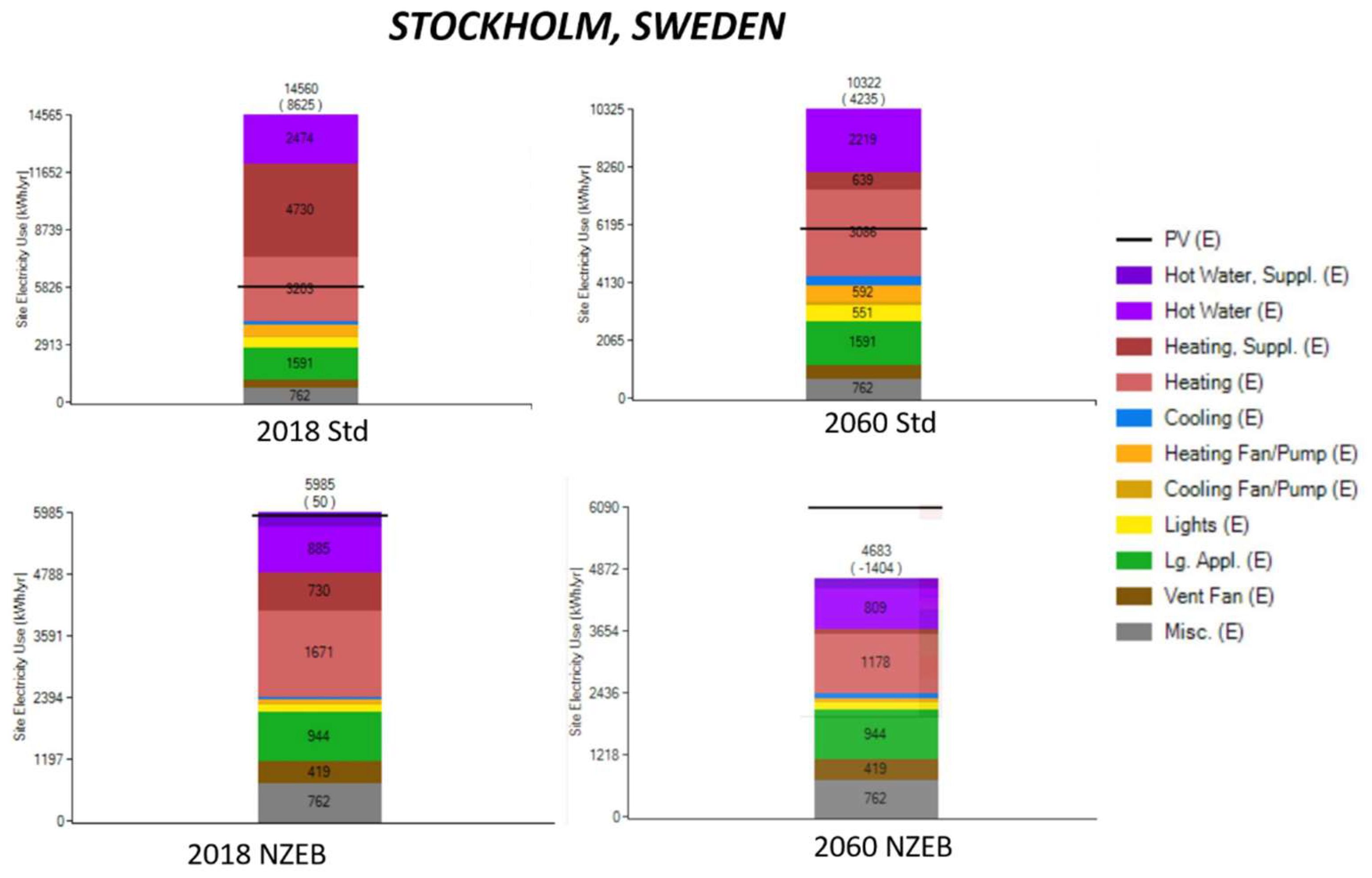
- Stockholm (Sweden)
- Milan (Italy)
- Vienna (Austria)
- Madrid (Spain)
- Paris (France)
- Munich (Germany)
- Lisbon (Portugal)
- Rome (Italy)
3. Methods
- the building is all-electric, in line with the EU strategy of a future electrification of the sector;
- an updated library of energy efficient options (envelope, appliances, systems) is included, in particular the building envelope generally has a long-term impact due to the differing lifetime time horizon;
- the cooling set points are set upwards to 25.6 °C for the control air node operative temperature in compliance with ISO Standard 7730;
- a standard air-source heat pump is selected with electric resistance and a seasonal coefficient of performance (SCOP = 2.4) evaluated at multiple temperature conditions in EN 14511 and EN 14825. The operating SCOP varies depending on both the prevailing temperature conditions and building characteristics;
- a more efficient heat pump (SCOP = 3.1) is also available. This system is often selected, particularly in extreme heating or cooling climates.
- ESavingn,i = energy savings within optimization iteration ‘n’ evaluated for option ‘i’.
- Base energyn = calculated energy use of the standard building at the beginning of iteration ‘n’.
- Measure energyn,i = estimated energy use of the base building with measure ‘i’ installed within iteration ‘n’.
- PV = total present-value of life-cycle costs before taxes;
- I = total first costs associated with energy saving measure;
- Vn = residual or salvage value at year n, the last year in the evaluation (50 years);
- a = single-present-value formula from j = 1 to n, and discount rate d; i.e., aj = (1 + d)−j;
- Mj = maintenance costs in year j;
- Rj = repair and replacement costs in year j;
- Pk = the initial price of the kth type of conventional energy carrier for energy types k = 1 to H;
- Qk = the quantity required of the kth type of energy;
- bj = a formula for finding the present value of an amount in the jth year, escalated at a rate Θk, where k denotes the kth type of energy carrier, and discounted at a rate d; i.e., bj = [(1 + Θk)/(1 + d)].
Author Contributions
Funding
Informed Consent Statement
Data Availability Statement
Acknowledgments
Conflicts of Interest
Appendix A


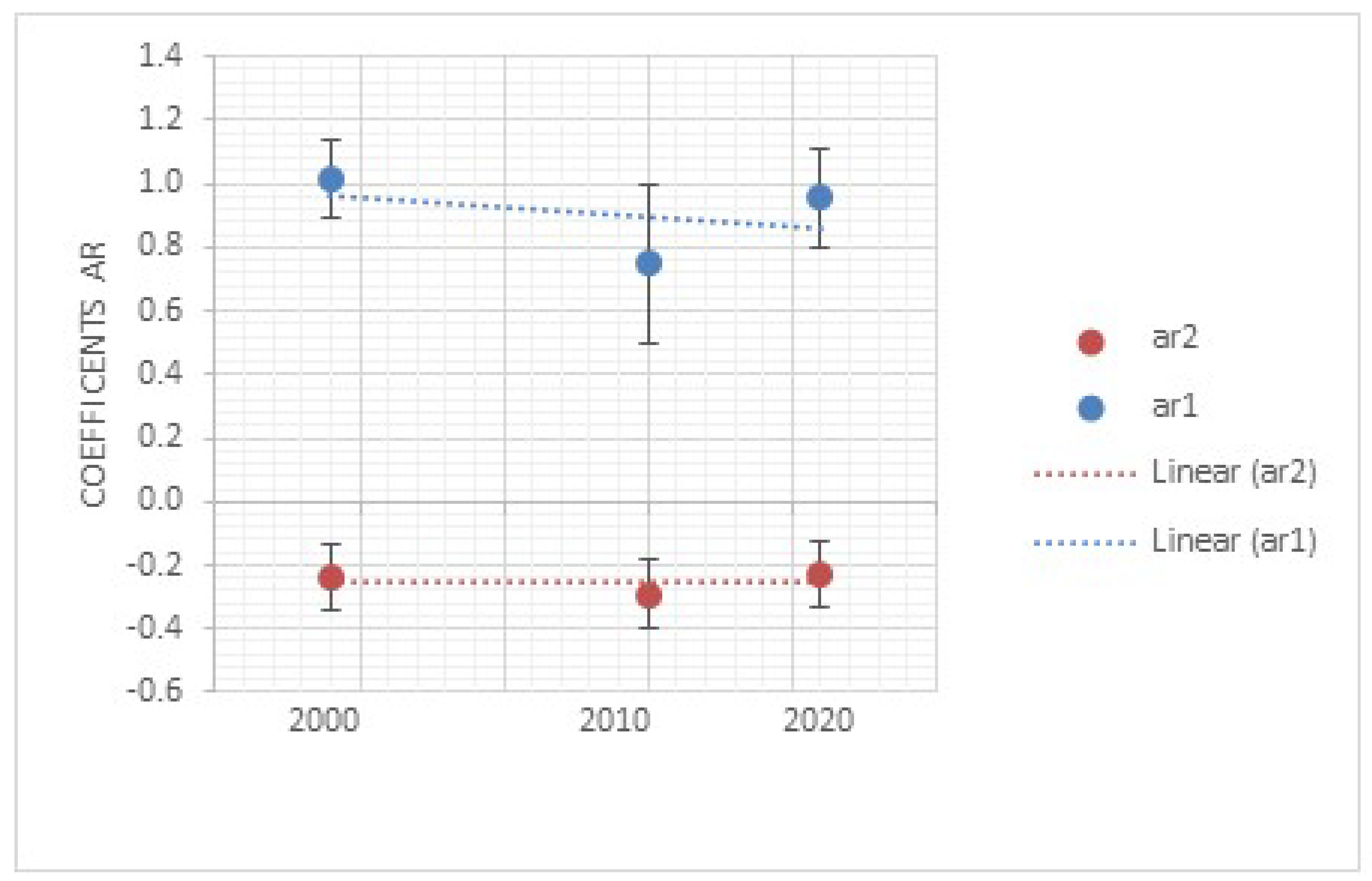
| AR1 | AR2 | MA1 | AIC | |
|---|---|---|---|---|
| 2000 | 1.0142 | −0.202 | −0.8887 | 1341.99 |
| 0.0606 | 0.0519 | 0.0368 | ||
| 2010 | 0.7496 | −0.2915 | −0.6754 | 1298.5 |
| 0.1249 | 0.0536 | 0.1292 | ||
| 2020 | 0.9577 | −0.2327 | −0.8307 | 1279.53 |
| 0.0773 | 0.0518 | 0.0632 |


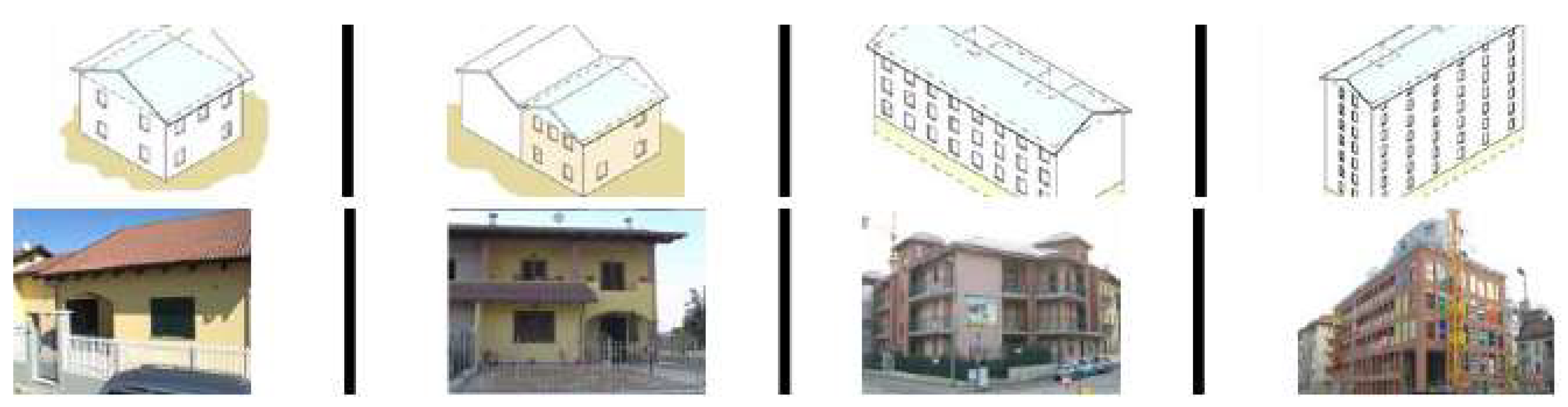
- Building 1: single-family house, characterized by a single real estate unit of an isolated type of one or two floors;
- Building 2: terraced house, characterized by a single real estate unit of one or two floors neighboring other housing units;
- Building 3: multi-family building characterized by a limited number of real estate units, from two to five floors and up to 15 apartments.
- Building 4: block of apartments, large building characterized by a higher number of real estate units.

| Standard | Heating | Cooling | ||
|---|---|---|---|---|
| Building effect | p-value | Test | p-value | Test |
| 2000 | 0.0027 | Building 4 | 0 | Building 3, Building 4 |
| 2010 | 0.0006 | Building 3 Building 4 | 0 | No-sign. difference |
| 2020 | 0.0101 | Building 4 | 0 | No-sign. difference |
| Year effect | ||||
| Building 1 | 0.0086 | 2000–2020 | 0.0979 | No-sign. difference |
| Building 2 | 0.0061 | 2000–2020 | 0.0015 | 2000 |
| Building 3 | 0.0177 | 2000–2020 | 0.0135 | 2020 |
| Building 4 | 0.0082 | 2000–2020 | 0.0016 | 2020 |
| NZEBs | ||||
| Building effect | p-value | p-value | ||
| 2000 | 0 | Building 1 | 0.5595 | No-sign. difference |
| 2010 | 0.1760 | Building 2 | 0.8892 | No-sign. difference |
| 2020 | 0.1760 | Building 2 | 0.8892 | 2020 |
| Year effect | ||||
| Building 1 | 0.1922 | 2020 | 0.9794 | No-sign. difference |
| Building 2 | 0.0177 | 2020 | 0.9609 | No-sign. difference |
| Building 3 | 0.6468 | 2020 | 0.9901 | No-sign. difference |
| Building 4 | 0.4642 | 2020 | 0.9990 | No-sign. difference |
References
- EC, REPowerEU: Joint European Action for More Affordable, Secure and Sustainable Energy. March 2022. Available online: https://ec.europa.eu/commission/presscorner/detail/en/fs_22_1938 (accessed on 14 April 2022).
- EC, the European Green Deal, COM (2019) 640 Final, Communication from the Commission to the European Parliament, the European Council, the Council, The European Economic and Social Committee and the Committee of the Regions. Available online: https://ec.europa.eu/info/sites/info/files/european-green-deal-communication_en.pdf (accessed on 29 March 2022).
- Economidou, M.; Todeschi, V.; Bertoldi, P.; D’Agostino, D.; Zangheri, P.; Castellazzi, L. Review of 50 years of EU energy efficiency policies for buildings. Energy Build. 2020, 225, 110322. [Google Scholar] [CrossRef]
- EU. Directive 2010/31/EU. European parliament and of the council of 19 May 2010 on the energy performance of buildings (recast). Off J. Eur. Union 2010, L 153/13. Available online: https://eur-lex.europa.eu/legal-content/EN/TXT/PDF/?uri=CELEX:32010L0031&from=EN (accessed on 29 March 2022).
- Revision of the Directive of the European Parliament and of the Council on the Energy Performance of Buildings (Recast), COM(2021) 802 Final. Available online: https://ec.europa.eu/energy/sites/default/files/proposal-recast-energy-performance-buildings-directive.pdf (accessed on 10 March 2022).
- Gaterell, M.R.; McEvoy, M.E. The impact of climate change uncertainties on the performance of energy efficiency measures applied to dwellings. Energy Build. 2005, 37, 982–995. [Google Scholar] [CrossRef]
- Herrera, M.; Natarajan, S.; Coley, D. A review of current and future weather data for building simulation. J. Build. Serv. Eng. Res. Technol. 2017, 38, 602–627. [Google Scholar] [CrossRef] [Green Version]
- Bot, K.; Ramos Nuno, M.M.; Almeida, R.M.S.F.; Pereira, P.F.; Monteiro, C. EO with on-site energy generation and storage—An integrated assessment using dynamic simulation. J. Build. Eng. 2019, 24, 100769. [Google Scholar] [CrossRef]
- Roberts, M.; Allen, S.; Coley, D. Life cycle assessment in the building design process—A systematic literature review. Build. Environ. 2020, 185, 107274. [Google Scholar] [CrossRef]
- Ferrara, M.; Fabrizio, E.; Virgone, J.; Filippi, M. A simulation based optimization method for cost-optimal analysis. Energy Build. 2014, 84, 442–457. [Google Scholar] [CrossRef]
- Österbring, M.; Mata, É.; Thuvander, L.; Mangold, M.; Johnsson, F.; Wallbaum, H. A differentiated description of building-stocks for a georeferenced urban bottom-up building-stock model. Energy Build. 2020, 120, 78–84. [Google Scholar] [CrossRef] [Green Version]
- Ganesh, H.S.; Seo, K.; Fritz, H.E.; Edgar, T.F.; Novoselac, A.; Baldea, M. Indoor air quality and energy management in buildings using combined moving horizon estimation and model predictive control. J. Build. Eng. 2021, 33, 101552. [Google Scholar] [CrossRef]
- Jeong, J.; Hong, T.; Ji, C.; Kim, J.; Lee, M.; Jeong, K.; Koo, C. Development of a prediction model for the cost saving potentials in implementing the building energy efficiency rating certification. Appl. Energy 2007, 189, 257–270. [Google Scholar] [CrossRef]
- Nägeli, C.; Jakob, M.; Catenazzi, G.; Ostermeyer, Y. Policies to decarbonize the Swiss residential building stock: An agent-based building stock modeling assessment. Energy Policy 2020, 146, 111814. [Google Scholar] [CrossRef]
- D’Agostino, D.; Parker, D. A framework for the cost-optimal design of nearly zero energy buildings (NZEBs) in representative climates across Europe. Energy 2018, 149, 814–829. [Google Scholar] [CrossRef]
- D’Agostino, D.; Parker, D. Data on cost-optimal Nearly Zero Energy Buildings (NZEBs) across Europe. Data Brief 2018, 17, 1168–1174. [Google Scholar] [CrossRef] [PubMed]
- Solomon, S. Climate Change 2007: The Physical Science Basis; Cambridge University Press: Cambridge, UK, 2007. [Google Scholar]
- Guan, L. Preparation of future weather data to study the impact of climate change on buildings. Build. Environ. 2009, 44, 793–800. [Google Scholar] [CrossRef]
- Robert, A.; Kummert, M. Designing Net Zero Energy Buildings for the Future Climate, not for the Past. Build. Environ. 2012, 55, 150–158. [Google Scholar] [CrossRef]
- D’Agostino, D.; Parker, D.; Epifani, I.; Crawley, D.; Lawrie, L. How will future climate impact the design and performance of Nearly Zero Energy Buildings (NZEBs)? Energy 2022, 240, 122479. [Google Scholar] [CrossRef]
- Belcher, S.E.; Hacker, J.N.; Powell, D.S. Constructing design weather data for future climates. Build. Serv. Eng. Res. Technol. 2005, 26, 49–61. [Google Scholar] [CrossRef]
- UNFCCC. Adoption of the Paris Agreement. Proposal by the President. In Proceedings of the Paris Climate Change Conference, Paris, France, 30 November–12 December 2015. [Google Scholar]
- IPCC. Climate Change 2014: Synthesis Report, 5th Assessment Report of the Intergovernmental Panel on Climate Change; Pachauri, R.K., Meyer, I.A., Eds.; IPCC: Geneva, Switzerland, 2014. [Google Scholar]
- Schwalm, C.R.; Spencer, G.; Duffy, P.B. RCP8.5 tracks cumulative CO2 emissions. Proc. Natl. Acad. Sci. USA 2020, 117, 19656–19657. [Google Scholar] [CrossRef]
- Eames, M.; Kershaw, T.; Coley, D. The appropriate spatial resolution of future weather files for building simulation. J. Build. Perform Simul. 2012, 5, 347–358. [Google Scholar] [CrossRef] [Green Version]
- De Wilde, P. The Implications of a Changing Climate for Buildings. Build. Environ. 2012, 55, 1–7. [Google Scholar] [CrossRef] [Green Version]
- Kapsomenakis, J.; Kolokotsa, D.; Nikolaou, T.; Santamouris, M.; Zerefos, S.C. Forty years increase of the air ambient temperature in Greece: The impact on buildings. Energy Convers. Manag. 2013, 74, 353–365. [Google Scholar] [CrossRef]
- D’Agostino, D.; Parker, D. How will climate alter efficiency objectives? Simulated impact of using recent versus historic European weather data for the cost-optimal design of nearly zero energy buildings (nzebs). In E3S Web of Conferences; EDP Sciences: Les Ulis, France, 2019; Volume 111, p. 04051. [Google Scholar] [CrossRef] [Green Version]
- ASHRAE. International Weather for Energy Calculations (IWEC and IWEC2 Weather Files) Users Manual and CD-ROM. In ASHRAE Transactions; PART 1; American Society of Heating, Refrigerating and Air Conditioning Engineers: Atlanta, GA, USA, 2001; Volume 112, pp. 226–240. [Google Scholar]
- Congedo, P.M.; Baglivo, C.; Zacà, I.; D’Agostino, D.; Quarta, F.; Cannoletta, A.; Marti, A.; Ostuni, V. Energy retrofit and environmental sustainability improvement of a historical farmhouse in Southern Italy. Energy Procedia 2017, 133, 367–381. [Google Scholar] [CrossRef]
- Huang, Y.J.; Crawley, D.B. Does it Matter Which Weather Data You Use in Energy Simulations? DOE-2 User News 1997, 18, 2–12. [Google Scholar]
- Crawley, D.B. Which Weather Data Should You Use for Energy Simulations of Commercial Buildings? In ASHRAE Transactions; ASHRAE: Atlanta, GA, USA, 1998; Volume 104, pp. 498–515. [Google Scholar]
- Crawley, D.B.; Lawrie, L.K. Should I Care How Old My Climate Data Is? In Proceedings of the CIBSE ASHRAE Technical Symposium, Glasgow, UK, 16–17 April 2020. [Google Scholar]
- Huld, T.; Paietta, E.; Zangheri, P.; Pinedo Pascua, I. Assembling Typical Meteorological Year Data Sets for Building Energy Performance Using Reanalysis and Satellite Based Data. Atmosphere 2018, 9, 53. [Google Scholar] [CrossRef] [Green Version]
- D’Agostino, D.; Mazzarella, L. What is a Nearly zero energy building? Overview, implementation and comparison of definitions. J. Build. Eng. 2019, 21, 200–212. [Google Scholar] [CrossRef]
- D’Agostino, D. Assessment of the progress towards the establishment of definitions of Nearly Zero Energy Buildings (NZEBs) in European Member States. J. Build. Eng. 2015, 1, 20–32. [Google Scholar] [CrossRef]
- Moazami, A.; Nik, V.M.; Carlucci, S.; Geving, S. Impacts of future weather data typology on building energy performance—Investigating long-term patterns of climate change and extreme weather conditions. Appl. Energy 2019, 238, 696–720. [Google Scholar] [CrossRef]
- WeatherShift. 2020. Available online: https://www.weathershift.com/ (accessed on 10 February 2022).
- Christensen, C.; Horowitz, S.; Givler, T.; Barker, G.; Courney, A. BEopt: Software for Identifying Optimal Building Designs on the Path to Zero Net Energy, NREL/CP-550-3733; National Renewable Energy Laboratory: Washington, DC, USA, 2005.
- Corrado, V.; Ballarini, I.; Corgnati, S.P. Building Typology Brochure, Italy; Pubblicazione Nell’ambito Del Progetto Tabula; GmbH: Darmstadt, Germany, 2014; ISBN 978-88-8202-065-1. Available online: https://episcope.eu/fileadmin/tabula/public/docs/brochure/IT_TABULA_TypologyBrochure_POLITO.pdf (accessed on 14 April 2022).
- Attia, S.; Gratia, E.; De Herde, A.; Hensen, J. Simulation-based decision support tool for early stages of zero-energy building design. Energy Build. 2012, 49, 2–15. [Google Scholar] [CrossRef] [Green Version]
- Tang, L.; Chen, C.; Tang, S.; Wu, Z.; Trofimova, P. Building Information Modeling and Building Performance Optimization. Encycl. Sustain. Technol. 2017, 311–320. [Google Scholar] [CrossRef]
- Wright, J.A.; Loosemore, H.A.; Farmani, R. Optimization of building thermal design and control by multi-criterion genetic algorithm. Energy Build. 2002, 34, 959–972. [Google Scholar] [CrossRef]
- UNI EN 15459. Energy Performance of Buildings, Economic Evaluation Procedure for Energy Systems in Buildings; CEN: Brussels, Belgium, 2008. [Google Scholar]
- Feist, W.; Pfluger, R.; Kaufmann, B.; Schnieders, J.; Kah, O. Passivhaus Projektierungs Paket 2004; Passivhaus Institut Darmstadt: Darmstadt, Germany, 2004. [Google Scholar]
- Lu, Y.; Wang, S.; Yan, C.; Huang, Z. Robust optimal design of renewable energy system in nearly/net zero energy buildings under uncertainties. Appl. Energy 2017, 187, 62–71. [Google Scholar] [CrossRef]
- Congedo, P.M.; Lorusso, C.; De Giorgi, M.G.; Marti, R.; D’Agostino, D. Horizontal air-ground heat exchanger performance and humidity simulation by computational fluid dynamic analysis. Energies 2016, 9, 930. [Google Scholar] [CrossRef] [Green Version]
- Eurostat, Final Energy Consumption by Sector. 2019. Available online: http://epp.eurostat.ec.europa.eu/portal/page/portal/statistics/search_database (accessed on 7 February 2022).
- EC. Directorate-General for Economic and Financial Affairs European Economic Forecast. Available online: http://ec.europa.eu/economy_finance/eu/forecasts/2015_spring_forecast_en.htm (accessed on 22 February 2022).
- Burch, J.; Christensen, C. Towards Development of an Algorithm to Predict Mains Water Temperature. In Proceedings of the 2007 American Solar Energy Society (ASES) Annual Conference, Cleveland, OH, USA, 8–12 July 2007. [Google Scholar]
- Zacà, I.; D’Agostino, D.; Congedo, P.M.; Baglivo, C. Data of cost-optimality and technical solutions for high energy performance buildings in warm climate. Data Brief 2015, 4, 222–225. [Google Scholar] [CrossRef]
- D’Agostino, D.; Cuniberti, B.; Bertoldi, P. Energy consumption and efficiency technology measures in European non-residential buildings. Energy Build. 2017, 153, 72–86. [Google Scholar] [CrossRef]
- D’Agostino, D.; Parker, D.; Melià, P.; Dotelli, G. Data on roof renovation and photovoltaic energy production including energy storage in existing residential buildings. Data Brief 2022, 41, 107874. [Google Scholar] [CrossRef] [PubMed]
- D’Agostino, D.; Tzeiranaki, S.T.; Zangheri, P.; Bertoldi, P. Data on nearly zero energy buildings (NZEBs) projects and best practices in Europe. Data Brief 2021, 39, 107641. [Google Scholar] [CrossRef] [PubMed]
- D’Agostino, D.; Parker, D.; Melià, P. Environmental and economic data on energy efficiency measures for residential buildings. Data Brief 2020, 28, 104905. [Google Scholar] [CrossRef]
- D’Agostino, D.; Mazzarella, L. Data on energy consumption and Nearly zero energy buildings (NZEBs) in Europe. Data Brief 2018, 21, 2470–2474. [Google Scholar] [CrossRef]
- D’Agostino, D.; Tzeiranaki, S.T.; Zangheri, P.; Bertoldi, P. Assessing Nearly Zero Energy Buildings (NZEBs) development in Europe. Energy Strategy Rev. 2021, 36, 100680. [Google Scholar] [CrossRef]
- Congedo, P.M.; Baglivo, C.; Zacà, I.; D’Agostino, D. High performance solutions and data for nZEBs offices located in warm climates. Data Brief 2015, 5, 502–505. [Google Scholar] [CrossRef]
- D’Agostino, D.; Parker, D.; Melià, P.; Dotelli, G. Optimizing photovoltaic electric generation and roof insulation in existing residential buildings. Energy Build. 2022, 255, 111652. [Google Scholar] [CrossRef]
- D’Agostino, D.; Cuniberti, B.; Bertoldi, P. Data on European non-residential buildings. Data Brief 2017, 14, 759–762. [Google Scholar] [CrossRef] [PubMed]
- D’Agostino, D.; Zacà, I.; Baglivo, C.; Congedo, P.M. Economic and thermal evaluation of different uses of an existing structure in a warm climate. Energies 2017, 10, 658. [Google Scholar] [CrossRef] [Green Version]
- D’Agostino, D.; Cuniberti, B.; Maschio, I. Criteria and structure of a harmonised data collection for NZEBs retrofit buildings in Europe. Energy Procedia 2017, 140, 170–181. [Google Scholar] [CrossRef]


| T | RH | GHI | DNI | DHI | IRD | WS | WD | P | |
|---|---|---|---|---|---|---|---|---|---|
| T | / | −0.24 | 0.46 | 0.32 | 0.43 | 0.85 | −0.07 | −0.008 | −0.15 |
| RH | / | −0.29 | −0.22 | −0.28 | −0.21 | −0.07 | −0.02 | 0.15 | |
| GHI | / | 0.89 | 0.77 | 0.33 | 0.16 | −0.11 | −0.006 | ||
| DNI | / | 0.47 | 0.16 | 0.11 | −0.11 | 0.07 | |||
| DHI | / | 0.37 | 0.15 | −0.05 | −0.09 | ||||
| IRD | / | 0.04 | 0.11 | −0.33 | |||||
| WS | / | −0.06 | −0.16 | ||||||
| WD | / | −0.07 | |||||||
| P | / |
| End Use | Annual kWh |
|---|---|
| Misc. (E) | 762.0 |
| Vent Fan (E) | 454.3 |
| Lg. Appl. (E) | 1591.5 |
| Lights (E) | 551 |
| Cooling Fan/Pump (E) | 187.6 |
| Heating Fan/Pump (E) | 442.6 |
| Cooling (E) | 524.6 |
| Heating (E) | 2230.4 |
| Heating, Suppl. (E) | 381.1 |
| Hot Water (E) | 2086.8 |
| Total | 9212 |
| PV | 7623 |
| Net (Total PV) | 1589 |
Publisher’s Note: MDPI stays neutral with regard to jurisdictional claims in published maps and institutional affiliations. |
© 2022 by the authors. Licensee MDPI, Basel, Switzerland. This article is an open access article distributed under the terms and conditions of the Creative Commons Attribution (CC BY) license (https://creativecommons.org/licenses/by/4.0/).
Share and Cite
D’Agostino, D.; Parker, D.; Epifani, I.; Crawley, D.; Lawrie, L. Datasets on Energy Simulations of Standard and Optimized Buildings under Current and Future Weather Conditions across Europe. Data 2022, 7, 66. https://0-doi-org.brum.beds.ac.uk/10.3390/data7050066
D’Agostino D, Parker D, Epifani I, Crawley D, Lawrie L. Datasets on Energy Simulations of Standard and Optimized Buildings under Current and Future Weather Conditions across Europe. Data. 2022; 7(5):66. https://0-doi-org.brum.beds.ac.uk/10.3390/data7050066
Chicago/Turabian StyleD’Agostino, Delia, Danny Parker, Ilenia Epifani, Dru Crawley, and Linda Lawrie. 2022. "Datasets on Energy Simulations of Standard and Optimized Buildings under Current and Future Weather Conditions across Europe" Data 7, no. 5: 66. https://0-doi-org.brum.beds.ac.uk/10.3390/data7050066