Wavelet Transforms of Diagnosable Signals from Ship Power Complexes in a MATLAB Environment


1
Department of Electrical Engineering and Automation, Admiral Makarov State University of Maritime and Inland Shipping, 198035 Saint-Petersburg, Russia
2
Department of Ship’s Electrical Equipment and Automatization, Kerch State Maritime Technological University, 298309 Kerch, Russia
3
Department of Cyber-Physical Systems, Saint Petersburg State Marine Technical University, Leninskiy Prosp., 101, 198303 Saint-Petersburg, Russia
*
Author to whom correspondence should be addressed.
Designs 2020, 4(4), 52; https://0-doi-org.brum.beds.ac.uk/10.3390/designs4040052
Submission received: 12 November 2020
/
Revised: 23 November 2020
/
Accepted: 25 November 2020
/
Published: 2 December 2020
Abstract
:The use of digital technologies in the systems of diagnostics and monitoring of units of a ship’s propulsion plant can significantly increase the efficiency and quality of assessing the technical condition of operated objects in the online mode as well as expand the class of practical problems to be solved. Digital processing of signals of complex configuration at a qualitatively new level is an indispensable condition for a critical improvement in the course of processing the current values of diagnosable parameters, increasing the reliability and trouble-free performance of a ship’s technical equipment during operation. A method of approximation has been discussed in the paper. Moreover, the paper provides an algorithm for analyzing the signal of the indicator diagram of a marine diesel engine, the spectrum of which contains high-frequency components and short-term pulses indicating deviations from the normal operating mode, the assessment of which is practically impossible with the traditionally applied methods of spectral analysis of signals. The approximation method is based on the use of wavelet analysis, which makes it possible to deeply explore such modes. Examples of using wavelet analysis to approximate one-dimensional signals of elements and systems of a ship’s power complexes are given.
1. Introduction
Online monitoring of the technical condition of technical facilities in operation in maritime transport is associated with digital processing of complex signals. The frequency spectrum of the analyzed signals, as a rule, contains the harmonic components of high frequencies, which are estimated on the Fourier basis. Evaluations are performed using hardware, including harmonic analyzers of various designs. Signals of complex configuration include voltages and currents of systems and elements of power complexes containing nonlinear semiconductor converters, sources of noise and vibrations during the operation of the main and auxiliary engines of a ship’s power systems, non-stationary vibrations of the ship’s hull structures in waves, shallow waterways, etc. They also include resonance vibrations that can occur on ships at certain speed modes of powerful energy converters. Signals of a complex configuration, along with the deterministic component, may contain interference, individual pulses with a weak energy spectrum. A wide variety of monitored signals creates conditions for improving the quality of diagnostics of the ship’s operating parameters, using digital technologies under the conditions of simultaneous use of machines and mechanisms which must be supplemented with tools for rapid signal analysis, since they may contain components containing information with signs of violations of the normal operating mode. These features include increased fuel consumption, changes in the temperature regimes of ship systems and mechanisms, the occurrence of vibration modes due to misalignment of the shafts as well as insufficient rigidity of the mountings of the units, and many more. In the modes of monitoring the technical condition, it is required to make decisions promptly, with retrieving the most complete information about the state of the object and assessing the type and location as well as the cause of a defect or malfunction in an automatic mode [1,2,3].
The task, here, is to create such algorithms and systems of technical diagnostics, which should, by individual signs and their combination, determine the likelihood of a malfunction in advance [1]. This will allow taking preventive measures to ensure trouble-free operation of a ship’s technical systems [1,2,3].
Maritime diesel installations (MDIs) are complex complexes consisting of many subsystems and units. During operation, complex chemical–physical processes and energy transformations take place in them. On the other hand, marine diesel installations during operation can be exposed to vibrations, shock loads, moisture, salt, changes in ambient temperature in a wide range, etc. Such influences accelerate the process of degradation of parts and assemblies of the MDIs and reduce their reliability. Maintaining the reliability of MDI operation during autonomous navigation of ships not only ensures the safety of the ship’s crew and cargo but also increases the economy and efficiency of the operation of ships. These goals can be achieved by monitoring the performance of installations and early detection of symptoms of a violation of their normal operation. This is the task of technical diagnostics of the MDI during operation. In general, technical diagnostics can include one or more of the following tasks:
- -
- Determination of the technical condition (performance) of the object;
- -
- Searching for a defect that has arisen;
- -
- Forecasting changes in the technical state of the object.
The theory of technical diagnostics systems in general, and for MDIs in particular, has arisen and developed since the 1970s in the works of world-renowned researchers. However, insufficient attention is paid to the development of technical means for diagnosing MDIs, which can assist a ship’s crew in assessing the technical condition of the power plant during autonomous navigation of ships [4,5,6].
Increasing requirements for the accuracy of diagnosing objects when processing signals with local impulses and other features leads to the necessity of improving the theory, methods, and techniques for assessing the technical state of a ship’s systems. Traditional methods based on the use of orthogonal series become ineffective for a profound and comprehensive analysis of signals with complex configurations, including cases when they are expanding into an orthogonal series using Fourier approximation. In practical calculations, an infinite number of terms in the Fourier series is not used, and the use of a limited number of harmonics leads to large errors [7]. In such cases, wavelet transform technologies can be considered very promising solutions [6]. A large package of wavelets, presented in modern computing systems, as well as a set of functions designed to process signals coming from information sensors, makes it possible to use them effectively to solve practical problems of monitoring and diagnosing the technical state of objects in steady-state and transient modes.
Wavelet technologies are developed on basic functions that preserve localization properties in the frequency and time domains [4]. They provide the implementation of high-precision algorithms for the approximation of one-dimensional and multidimensional characteristics.
2. Methods and Materials
High-precision approximation procedures in quasi-static modes during the working cycle are required to be used when measuring the pressure, temperature, weight, and composition of exhaust gases in a diesel cylinder. High-precision technologies are required when studying the appearance of local zones while nitrogen oxides are being generated at various speed modes, researching the correlation properties of fuel combustion products by indirect methods, for producing data arrays obtained using indicator diagrams, and creating “reference” characteristics of technological processes. In this case, information can be stored in the form of arrays of wavelet transform coefficients, and cluster models can constitute a tool for invariants. Parameters beyond the boundaries set by the cluster can serve as a sign of deviation of the diagnosable parameter from the standard one.
Studies have shown that the frequency properties of indicator devices can significantly affect the frequency characteristics of the indicator channel, which leads to distortion of signals and increasing the error in assessing the indicators of the working process [8].
The digitalization of processes in the Fourier basis has shown that with Fourier series, it is difficult to detect local signals in the form of short pulses of a small amplitude, which may indicate the development of deviations of controlled signals from the standard ones against the background of measurements [9,10].
Wavelet analysis is a tool for studying signals with local features. Wavelets and wavelet transforms allow for obtaining spectrograms of signals with local features. It is easy to determine their location in the amplitude-time domain, which is practically impossible to perform in the Fourier basis [5]. Wavelet transforms are based on modern digital technologies, the implementation of which requires the use of tools of modern computing systems containing a set of functions with established syntactic rules.
The MATLAB Wavelet Toolbox contains a list of basic wavelets, such as Haar, Morlet, Meyer, Shannon, Daubechies, frequency B-spline, etc. The Haar and Daubechies wavelets are most widely used in practice, having a lot in common in information coding [2]. In this regard, the Haar wavelet in the packet is denoted by the symbol db1, and the Daubechies wavelets can be selected from the db2, db3, …, db10 family, represented by nine wavelets. Modification of Daubechies wavelets allows for an increase in the symmetry properties of filters while maintaining the simplicity of working with them [11].
Wavelet transforms are designed to process large amounts of information. At the same time, their technologies and algorithms are suitable for working with simple signals that allow one to observe, step by step, the progress of transformations carried out by the algorithm. Let us consider the following example of this mode.
Suppose that the measurements of the hourly fuel consumption during the progress of a vessel with a displacement of 2000 tons during 8 running hours were (kg/h) as follows:
y = (152 154 156 157 156 157 158 156).
By delta coding, we will obtain an approximation of the fuel consumption vector y using the “db1” wavelet. For this purpose, according to the Haar transformation, we split the elements of the vector y into pairs and determine the half-sum and half-difference of values in each of them. We define the half-sums and half-differences using the matrix R of the following form:
R = (1/2 1/2 0 0 0 0 0 0;−1/2 1/2 0 0 0 0 0 0;0 0 1/2 1/2 0 0 0 0;0 0 −1/2 1/2 0 0 0 0;
0 0 0 0 1/2 1/2 0 0;0 0 0 0 −1/2 1/2 0 0;0 0 0 0 0 0 1/2 1/2;0 0 0 0 0 0 −1/2 1/2).
0 0 0 0 1/2 1/2 0 0;0 0 0 0 −1/2 1/2 0 0;0 0 0 0 0 0 1/2 1/2;0 0 0 0 0 0 −1/2 1/2).
Vector f = R × y’ = (153.0 1.0 156.5 0.5 156.5 0.5 157.00 −1.0)T contains mean values of groups (half-sum) and half-difference. Next, from the mean values, we form the row vector Fcp = (f (1) f (1) f (3) f (3) f (5) f (5) f (7) f (7)) and use it to obtain deviations for the group elements from mean values:
r = y − Fcp = (−1.0000 1.0000 −0.5000 0.5000 −0.5000 0.5000 1.0000 −1.0000).
The vectors Fcp and r can also be obtained using the Haar wavelet transform for one-step signal decomposition using the “db1” wavelet, for which we use the following operators contained in the Wavelet Toolbox:
- [cA1,cD1] = dwt(y,‘db1’).As a result, we will havecA1 = (216.3747 221.3244 221.3244 222.0315),cD1 = (−1.4142 −0.7071 −0.7071 1.4142).
- A1 = upcoef(‘a’,cA1,‘db1’,1,ls); D1 = upcoef(‘d’,cD1,‘db1’,1,ls).
The upcoef operator is used to approximate A1 and refine D1 of the first wavelet transform level by the obtained vectors cA1 and cD1. The identity of the estimates is determined by the fact that A1 = Fcp and D1 = r. According to the syntax of the operator, the following ones are sequentially given in parentheses: the symbols ‘a’ and ‘d’, specifying which kind of decomposition should be performed; vector cA1 is introduced for approximation, and vector cD1 for refining; Daubechies wavelet with the corresponding number ‘db1’ is selected; the number of the operation level is entered—for example, 1; the number of elements of the vector of the processed signal ls is indicated (for the vector y, the value ls = 8).
Now, we will turn our attention to the operator [cA1, cD1] = dwt (y, ‘db1’). As applied to the example under consideration, the operator performs a linear transformation of each group of two elements of the vector yc using the rotation matrix M consisting of the following elements:
M = [1/sqrt(2) 1/sqrt(2);−1/sqrt(2) 1/sqrt(2)].
As a result, the elements of vectors cA1 and cD1 are determined. In particular, we have, element by element, for four groups:
[cA1(1) cD1(1)]′ = M × [y(1) y(2)]′ = [216.3747 1.4142]′;
[cA1(2) cD1(2)]′ = M × [y(3) y(4)]′ = [221.3244 0.7071]′;
[cA1(3) cD1(3)]′ = M × [y(5) y(6)]′ = [221.3244 0.7071]′;
[cA1(4) cD1(4)]′ = M × [y(7) y(8)]′ = [222.0315 −1.4142]′.
The Haar transform is normalized using the matrix M, since the determinant of the matrix is det (M) = 1.0000. Therefore, when a pair of numbers rotates, the area of the normalized object does not change, i.e., information is not lost, which makes it possible to process the vector y by the formed pairs of numbers independently of each other. In the MATLAB environment, such a transformation is carried out using a block matrix consisting of blocks M in the main diagonal. Such a matrix can be obtained if the matrix R is multiplied, element by element, by sqrt (2):
W = R × sqrt(2).
Note that det(R) = 0.0625 with the determinant of every block 8 × det(R) = 0.5, while
det(W) = 1.0000.
The rows of the matrix M have orthogonality properties.
Let m1 = M(1,:) и m2 = M(2,:). Then, m1 × m1T = 1,m2 × m2T = 1 иm1 × m2T = 0.m2 × m1T = 0.
As a result, inv(W) = WT, and the inverse of the matrix can be obtained using the transpose operation.
Thus, vectors A1 and D1, obtained by the Haar transform, are two filters that separate the signal into low-frequency and high-frequency components (Figure 1). Low-frequency resolution characterizes signal power and high-frequency resolution characterizes its frequency associated with short pulses (bursts).
A person at the modern level of development of technology and its automation, due to the limited psychophysiological capabilities of a human individual in difficult conditions, cannot always find a managerial action adequate for a problematic or other operational situation. This is especially pronounced on modern ships with a high level of automation, when the navigator must almost instantly make decisions aimed at meeting the many requirements put forward by the operational situation (safety of navigation, energy savings, environmental safety, etc.). Another example is the impossibility of a representative of the organization for the classification and survey of ships for a relatively short survey period to completely check the technical condition of a ship and its elements, or at least all elements of the power plant (EPP) of the ship (in reality, the method of selective control, as a result of which the technical condition of a significant part of the EPP facilities turns out to be untested) (Figure 1). It is here that digital technologies based on knowledge in various fields of technology and the experience of specialists—in other words, artificial intelligence—should replace the intelligence of a human operator, which cannot always cover and evaluate a multi-level problem in its entire multidimensional difficulties.
Now, let us restore y. We perform signal regeneration using the wavelet transform inversion:
Ym = idwt(cA1, cD1,‘db1’,ls) = [152.00 154.00 156.00 157.00 156.00 157.00 158.00 156.00].
3. Mathematical and Software Implementation
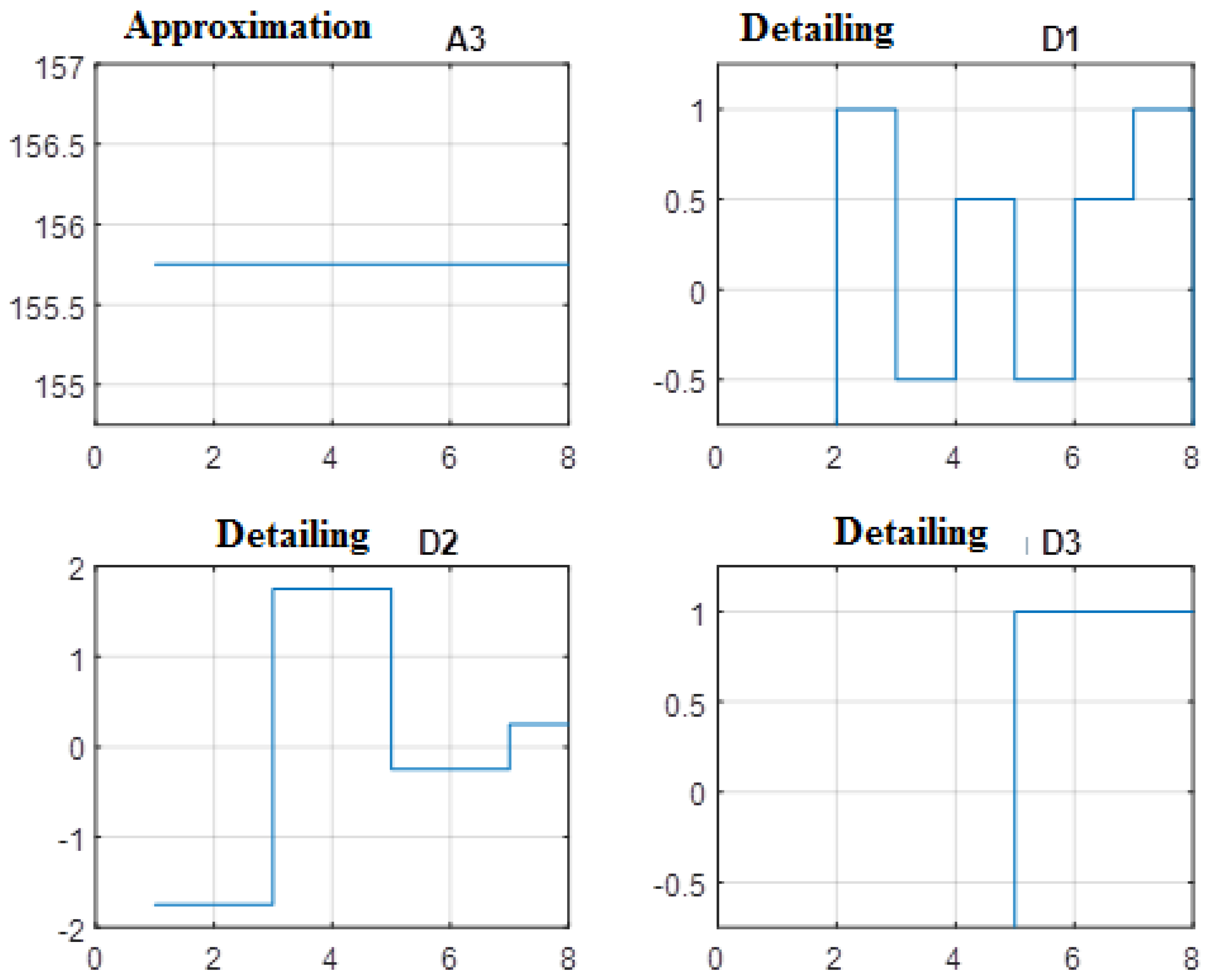
With multilevel processing of signals of a complex configuration based on the ‘db1’ wavelet, it is possible to guarantee an increase in the conversion quality due to a larger volume of digitalization of the process [8]. For definiteness, we perform the decomposition of y at detail level three (Figure 2). Then,
[C,L] = wavedec(y,3,‘db1’)
C = [440.5275 −2.8284 −3.5000 −0.5000 −1.4142 −0.7071 −0.7071 1.4142],
L = (1 1 2 4 8).
Using the obtained vectors C and L, using the appcoef function, we estimate the coefficient cA3 of the third level of approximation and detail. Observing the syntax, we obtain:
and for refining at levels 3, 2, and 1, we will have:
cA3 = appcoef(C,L,‘db1’,3) = 440.5275,
cD3 = detcoef(C,L,3) = −2.8284,
cD2 = detcoef(C,L,2) = [ −3.5000 −0.5000], cD1 = detcoef(C,L,1) = [−1.4142 −0.7071 −0.7071 1.4142].
Daubechies wavelets of the ‘db2’, …, ‘db10’ families in the Wavelet Toolbox are formed according to a different principle of forming groups of number sequences, which significantly improves the signal conversion process. Instead of groups with two points, for example, four points are taken with the shift of the elements of the subsequent group at each step by two elements to the left. For the vector y, such groups are as follows:
[y(1) y(2) y(3) y(4)], [y(3) y(4) y(5) y(6)],
[y(5) y(6) y(7) y(8)], [y(7) y(8) y(1) y(2)].
[y(5) y(6) y(7) y(8)], [y(7) y(8) y(1) y(2)].
Now, when realizing the low-pass and high-pass filters, each group of four numbers will be replaced by two numbers. Let the values of the elements of the vector y in the group be equal to x, v, z, and t. Then, we write the first filter as follows:
a = c1 × x + c2 × v + c3 × z + c4 × t.
The second filter d is represented by a linear model
d = c4 × x − c3 × v + c2 × z − c1 × t.
Such a permutation of elements provides the orthogonality property of the block Daubechies transformation matrix, which has the form:
DB = [c1 c2 c3 c4 0 0 0 0;
c4 −c3 c2 −c1 0 0 0 0;
0 0 c1 c2 c3 c4 0 0;
0 0 c4 −c3 c2 −c1 0 0;
0 0 0 0 c1 c2 c3 c4;
0 0 0 0 c4 −c3 c2 −c1;
c3 c4 0 0 0 0 c1 c2;
−c2 c1 0 0 0 0 −c4 c3].
To calculate the numerical values of the elements of the DB matrix, four equations are required. The first equation can be determined by the requirement of orthogonality
c1*c3 + c2*c4 = 0.
- It must be true for all linear pairs. The other three equations are determined by the requirements of the Daubechies transform.
- The sum of the squares of the coefficients must be equal to onesince for a single determinant, DB will also be equal to one.c1^2 + c2^2 + c3^2 + c4^2 = 1,
- Transformfor any equal k—for example, k = 1, it must take zero values.k*c4 − k*c3 + k*c2 − k*c1 = 0
- For linearly increasing values of m, for example, m = (1 2 3 4),Transformmust also take zero values.m(1)*c4 − m(2)*c3 + m(3)*c2 − m(4)*c1 = 0
The solution of the system of nonlinear Equations (2)–(5) is possible only by numerical methods. For this purpose, we will use the fsolve function in the Optimization Toolbox of the MATLAB package. Here is a fragment of the solution, with the account of the function syntax.
For this purpose, we introduce the following notation:
x(1) = c1, x(2) = c2, x(3) = c3, x(4) = c4.
Let us compose the file function sah568hh.m with Equations (2)–(5):
function F = sah568hh(x);
F = [x(1)^2 + x(2)^2 + x(3)^2 + x(4)^2 − 1;x(1)*x(3) + x(2)*x(4);−x(1) + x(2) − x(3) + x(4);−4*x(1) + 3*x(2) − 2*x(3) + x(4)].
Note that the ultimate goal of solving F is to turn the rows of the matrix equation back to “zero”, which creates certain convenience while working with the function. The function is called at each iteration from the main file sah568h.m, a fragment of which contains the initial approximation vector x0, options for displaying the solution on the display, and the fsolve function. Upon completion of the search for a solution, the vector x and the criterion for evaluating fval are displayed (Table 1):
% sah568h.m
x0 = [0.2 0.2 0.2 −0.2]’;
options = optimset(‘Display’,‘iter’);
[x,fval] = fsolve(‘sah568hh’,x0,options)
Iteration process
Equation is solved.
Output data:
x = [0.4830 0.8365 0.2241 −0.1294]T, fval = 1.0 × 10−11 *[0.7154 0.2126 0.0000 −0.0000].
Substituting the numerical values of the elements of the vector x into Equation (1), we obtain the determinant of the Daubechies matrix equal to det (DB) = 1.0000, as well as the condition DB−1 = DBT, which indicates the accuracy of the solutions performed.
To produce Daubechies wavelets, a greedy algorithm is used, which makes it possible to establish a scaling (refinable) function element-by-element if known coefficients are available and to select local features of the approximated signals. It is advisable to work with wavelet transforms with a high dimension of the analyzed signals according to the following Algorithm 1:
| Algorithm 1 Approximation of the Input Signal |
| 1. Signal loading. |
| 2. Spline—an approximation of the input signal. |
| 3. Assignment of the wavelet decomposition level. |
| 4. Wavelet selection. |
| 5. Decomposition of the signal with the determination of the approximating and refining components. |
| 6. Signal recovery by wavelet inversion-transform. |
| 7. Estimation of the first-level approximation error. |
| 8. Performing multilevel wavelet decomposition with the selection of approximation and refining coefficients. |
| 9. Reconstruction of the third-level approximation. |
| 10. Reconstruction of details of 1, 2, and 3 levels. |
| 11. Display of the produced components on the display. |
| 12. Analysis of the results of wavelet transforms and ensuring the noise immunity of signals. |
According to the algorithm, we will perform a wavelet analysis of the characteristics of the pressure change in the cylinder of a marine diesel engine at the nominal mode, obtained experimentally by taking the indicator diagram. To indicate a diesel engine, an indicator was used, which made it possible to record a diagram expanded along the angle of rotation of the crankshaft, which was used for wavelet analysis.
The analysis and synthesis of the diagram were performed using the sah568f.m file in MATLAB codes, where the points of the algorithm being implemented are also indicated by numbers. The file is compiled according to the given Algorithm 2. The data of the indicator diagram after appropriate processing is represented by a matrix of Z dimensions (73 × 2). The increase in the accuracy of the experimental data input is provided by the use of splines with a discreteness step of 0.5 deg. As a result, the pressure vector P of dimension (1 × 721). In our experiment, we will use the popular pressure sensor (OWEN PD100-DI sensors models 111, 171, 181) [12,13,14,15]. The characteristics of the pressure sensor used to obtain experimental data, such as resolution and sampling rate, are presented in the program listing and Figure 3 and Figure 4.
| Algorithm 2 Wavelet—Process Diagnostics |
| % sah568f.m |
| % Wavelet—process diagnostics. |
| %======================================================= |
| % The first step of the algorithm |
| load Z |
| % The second step of the algorithm. |
| fi1 = −160:0.5:200; |
Pcs = spline(Z(:,1),Z(:,2),fi1);
|
| fi = −160:0.5:200; |
| % Generation of the vector of P-dimension (1 × 721) |
P = [Pcs];
|
| % Overlay of the interference f on P signal as two spikes. |
| a = 0.1; b = 0.3; |
f = [zeros(1,500) (b − a)*rand(1,3) + a zeros(1,100) 0.3 zeros(1,117)];
|
| P = P + f; |
| v = size(P); |
| s = P(1:v(2)); |
| ls = length(s); |
| % The third and fourth steps in the algorithm |
| % Level 1, Daubechies wavelet ‘db1’. Transform algorithm Sm1 = A1 + D1 |
| [cA1,cD1] = dwt(s,‘db1’); |
| % The fifth step in the algorithm |
| A1 = upcoef(‘a’,cA1,‘db1’,1,l_s); |
| D1 = upcoef(‘d’,cD1,‘db1’,1,l_s); |
| % The sixth step in the algorithm |
| Sm1 = idwt(cA1,cD1,‘db1’,l_s); |
| % The seventh step in the algorithm |
| err = max(abs(s-Sm1)); |
| % The eighth step in the algorithm |
| [C,L] = wavedec(s,3,‘db1’); |
| cA3 = appcoef(C,L,‘db1’,3); |
| cD3 = detcoef(C,L,3); |
| cD2 = detcoef(C,L,2); |
| cD1 = detcoef(C,L,1); |
| [cD1,cD2,cD3] = detcoef(C,L,(1,2,3)); |
| % The ninth step in the algorithm |
| A3 = wrcoef(‘a’,C,L,‘db1’,3); |
| D1 = wrcoef(‘d’,C,L,‘db1’,1); |
| D2 = wrcoef(‘d’,C,L,‘db1’,2); |
| D3 = wrcoef(‘d’,C,L,‘db1’,3); |
| Sm3 = waverec(C,L,‘db1’); |
| err = max(abs(s-Sm3)) |
| % Error: |
| % err = 4.9738 × 10⁻¹⁴. |
| % The tenth and eleventh steps in the algorithm |
| subplot(2,2,1); plot(fi,A3);grid; title(‘Approximation level 3’); |
| subplot(2,2,2); plot(fi,D1);grid; title(‘Refining level 1’); |
| subplot(2,2,3); plot(fi,D2);grid; title(‘‘Refining level 2’); |
| subplot(2,2,4); plot(fi,D3);grid; title(‘Refining level 3’); |
| % The twelfth step in the algorithm |
| [thr,sorh,keepapp] = ddencmp(‘den’,‘wv’,s); |
| Sm = wdencmp(‘gbl’,C,L,‘db1’,3,thr,sorh,keepapp); |
| subplot(2,1,1); plot(fi,P),grid; title(‘Original’) |
| subplot(2,1,2); plot(fi,Sm),grid; title(Wavelet-model’) |
With a three-step approximation, as per the scheme
the maximum error was estimated by the formula
Sm3 = A3 + D1 + D2 + D3
err = max(abs(s-Sm3)) = 6.2172 × 10⁻¹⁵.
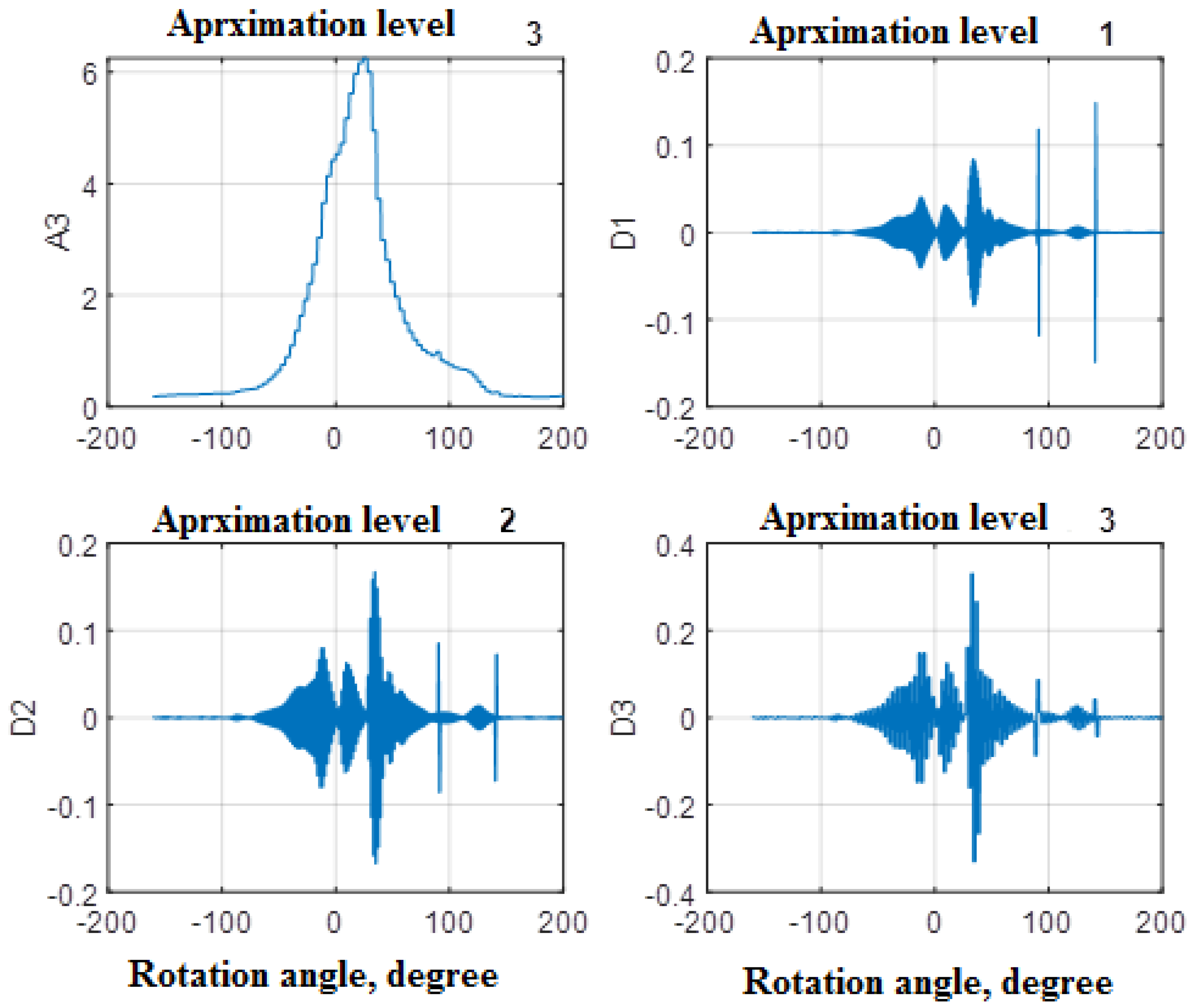
The graphs of the coefficients for the three-level decomposition are shown in Figure 3.
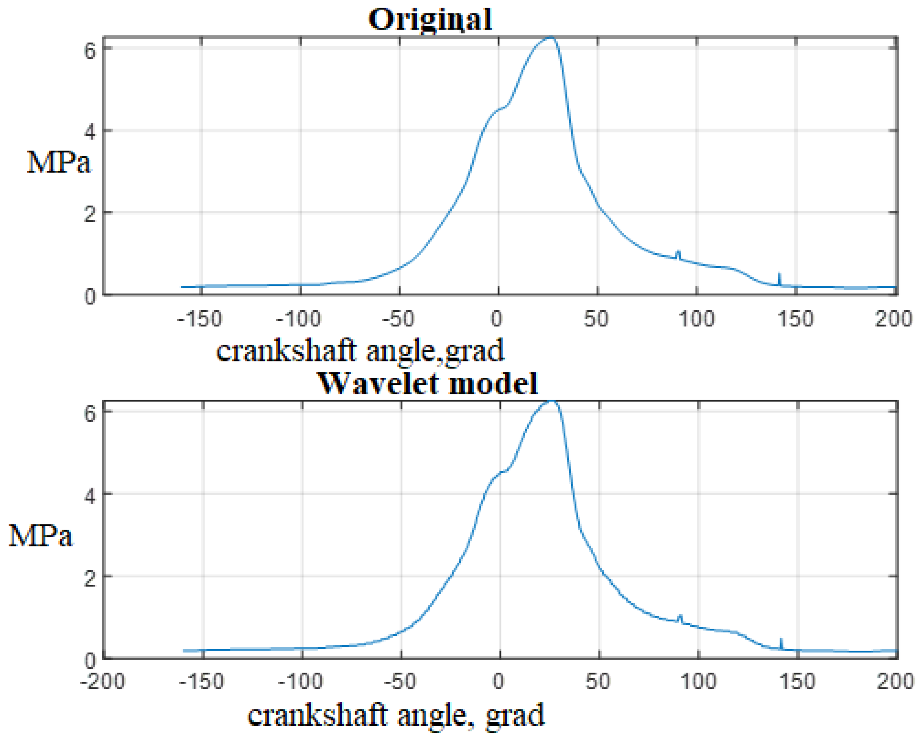
The inverse wavelet transform is implemented using the signal reconstruction functions provided in the file. Figure 4 shows the original and recovered signal characteristics. It can be seen that two “spikes” in the original characteristic are also displayed in the model generated by the inverse wavelet transform.
4. Discussion
Wavelet transforms are a modern signal-processing mechanism applicable for diagnosing the characteristics of elements and systems of a ship’s power complexes. Wavelets are a special class of functions with orthogonal properties, capable of performing shift and scaling (stretch/shrink) operations. The Haar and Daubechies wavelets are most commonly used in practice. Any wavelet generates a complete orthogonal system of functions. Wavelet analysis of the signal allows one to evaluate the differences in characteristics. Due to the property of completeness of the wavelet transform, it is possible to carry out recovery (reconstruction or synthesis) of the process with an estimate of the error. The “technology” of processing one-dimensional signals using Haar and Daubechies wavelets is considered. Other solutions remain at the discussion stage, in application to diagnostics of the technical condition of ship electrical complexes and ship automation systems based on new effective wavelet transformations, which should be the subject of further research.
The classification of signs and parameters of the technical condition of marine diesel engines has been made. The diagnostic parameters are differentiated by the level of information content. The ways of using information content when choosing the minimum set of diagnostic indicators that provide a given accuracy and reliability of diagnosis are shown [15,16].
The statement about increasing the accuracy of experimental data using the spline interpolation function was worked out in a specialized laboratory of the university on official licensed software.
5. Conclusions
- Wavelet transforms of one-dimensional discrete signals based on Haar and Daubechies wavelets consist of determining the parameters of low-pass and high-pass filters for expansion in a basis constructed with a wavelet by means of scale changes and transfers. Each of the basis functions characterizes its spatial (temporal) frequency and localization in physical space (time).
- For a simple signal consisting of eight measurements of the hourly fuel consumption, a method of dividing into groups is proposed, making it possible to obtain a Daubechies matrix of dimensions (8 × 8). The determinant of the matrix is equal to one, and the orthogonal properties made it possible to ensure the equality of the transposed and inverse Daubechies matrices.
- The elements of the Daubechies matrix were determined by numerically solving a system of nondelinear equations in the MATLAB environment, for which a file function was compiled that allows the “zeroing” of matrix rows containing the conditions of orthogonalization and consistency of the determinant.
- In parallel, calculations were performed using the functions of the Wavelet Toolbox package, which confirmed the accuracy of the transforms and solutions during the expansion and synthesis of the original function.
- An algorithm was developed for working with one-dimensional discrete signals, i.e., vectors of large dimensions. This algorithm is used for the wavelet transform of pressure in the cylinder of a marine diesel engine. Two “spikes” were introduced into the signal containing the numerical values of the pressure at the points of information retrieval, which, along with the main signal, were reconstructed using the components of the three-level approximation A3 and the details D1, D2, and D3.
- It is shown that in order to improve the efficiency of work with wavelet transforms, it is necessary to study the processes in relation to specific objects.
- The main objective of wavelet analysis in diagnosing and monitoring a ship’s power systems is to establish relevance between the standard evaluation criteria and wavelet coefficients.
Author Contributions
V.S., Methodology, Supervision; S.C. Formal analysis, Methodology; S.S., Resources; A.C. original draft. All authors have read and agreed to the published version of the manuscript.
Funding
The research is partially funded by the Ministry of Science and Higher Education of the Russian Federation as part of World-class Research Center program: Advanced Digital Technologies (contract No. 075-15-2020-903).
Conflicts of Interest
The authors declare no conflict of interest.
References
- Akhmetkhanov, R.S. Application of wavelet transforms for the analysis of one-, two- and three-dimensional data arrays. Problems of mechanical engineering and machine reliability. J. Mach. Manuf. Reliab. 2013, 42, 432–438. [Google Scholar] [CrossRef]
- Bestuzheva, A.P.; Lezin, A.P. Comparison of approximation capabilities of Haar and Daubechies wavelets. Perspective information technologies (PIT 2017). Intern. Sci. Technol. Conf. 2017, 2, 45–48. [Google Scholar]
- Guericke, B.L.; Guericke, P.B.; Shakhmanov, V.N. Fundamentals of dynamic diagnostics of machine units of mining equipment. Mining information and analytical bulletin. Sci. Technol. J. 2011, 3, 367–377. [Google Scholar]
- Dyakonov, V.P. Wavelets. In From Theory to Practice; SOLON-Press: Moscow, Russia, 2004; p. 448. [Google Scholar]
- Privalov, M.V.; Skobtsov, Y.A.; Kudryashov, A.G. Segmentation of Computer Tomograms Based on Wavelet Transform; Bulletin of the Kherson National Technical University: Kherson, Ukraine, 2009; pp. 31–36. [Google Scholar]
- Smolentsev, N.K. Fundamentals of the Theory of wavelets. In Wavelets in MATLAB, 4th ed.; Book on Demand Ltd.: Warsaw, Poland, 2014; p. 628. [Google Scholar]
- Travin, M.G. Wavelets for Engineers. Politerra 2007, 1, 423. [Google Scholar]
- Welstead, S. Fractals and Wavelets for Image Compression in Action; Publishing House Triumph: Moscow, Russia, 2003; p. 320. [Google Scholar]
- Daubechies, I. Ten Lectures on Wavelets. Regul. Chaotic Dyn. 1993, 1671. [Google Scholar] [CrossRef]
- Fedorov, V.M. Signal Segmentation Based on Discrete Wavelet Transform. In Information Counteraction to Terrorist Threats; Fedorov, V.M., Yurkov., P.Y., Eds.; Publishing house of TTI SFU: Taganrog, Russia, 2009; pp. 138–146. [Google Scholar]
- Stark, G.G. Application of wavelets for DSP. Technosphere 2007, 1, 183. [Google Scholar]
- Lee, G.; Wasilewski, F.; Gommers, R.; Wohlfahrt, K.; O’Leary, A.; Nahrstaedt, H. PyWavelets: Wavelet transforms in python. Pywavelets-Wavelet Transform. Python 2006, 2, 322. [Google Scholar]
- Wasilewski, F. PyWavelets-wavelet Transforms in Python. Available online: http://www.pybytes.com/pywavelets (accessed on 1 May 2010).
- Sokolov, S.; Zhilenkov, A.; Chernyi, S.; Nyrkov, A.; Glebov, N. Hybrid neural networks in cyber physical system interface control systems. Bull. Electr. Eng. Inf. 2020, 9, 1268–1275. [Google Scholar] [CrossRef] [Green Version]
- Zhilenkov, A.; Chernyi, S.; Sokolov, S.; Nyrkov, A. Intelligent autonomous navigation system for UAV in randomly changing environmental conditions. J. Intell. Fuzzy Syst. 2020, 1–7. [Google Scholar] [CrossRef]
- Avdeev, B.; Dema, R.; Chernyi, S. Study and Modeling of the Magnetic Field Distribution in the Fricker Hydrocyclone Cylindrical Part. Computation 2020, 8, 42. [Google Scholar] [CrossRef]
Figure 1.
Application of the wavelet ‘db1’ for single-level vector processing y.

Figure 2.
Three-level wavelet decomposition of the vector y based on the ‘db1’ wavelet.

Figure 3.
Graphs of coefficients of approximation and refining at three-level decomposition of the indicator diagram.
Figure 3.
Graphs of coefficients of approximation and refining at three-level decomposition of the indicator diagram.

Figure 4.
Pressure in the cylinder of a marine internal combustion engine: original and wavelet model.
Figure 4.
Pressure in the cylinder of a marine internal combustion engine: original and wavelet model.


Table 1.
Calculation parameters and metrics.
| Iteration | Func-Count | Func-Count f(x) | First-Order Step | Trust-Region Optimality | Radius |
|---|---|---|---|---|---|
| 0 | 5 | 1.5056 | 3.26 | 1 | |
| 1 | 10 | 0.561778 | 1 | 1.49 | 1 |
| 2 | 15 | 0.0147536 | 0.34671 | 0.211 | 1 |
| 3 | 20 | 1.35599 × 10⁻⁵ | 0.0599432 | 0.00592 | 1 |
| 4 | 25 | 1.35599 × 10⁻⁵ | 0.00207056 | 7.01 × 10⁻⁶ | 1 |
| 5 | 30 | 5.56834 × 10⁻²³ | 2.66337 × 10⁻⁶ | 1.17 × 10⁻¹¹ | 1 |
Publisher’s Note: MDPI stays neutral with regard to jurisdictional claims in published maps and institutional affiliations. |
© 2020 by the authors. Licensee MDPI, Basel, Switzerland. This article is an open access article distributed under the terms and conditions of the Creative Commons Attribution (CC BY) license (http://creativecommons.org/licenses/by/4.0/).
Share and Cite
MDPI and ACS Style
Sakharov, V.; Chernyi, S.; Saburov, S.; Chertkov, A. Wavelet Transforms of Diagnosable Signals from Ship Power Complexes in a MATLAB Environment. Designs 2020, 4, 52. https://0-doi-org.brum.beds.ac.uk/10.3390/designs4040052
AMA Style
Sakharov V, Chernyi S, Saburov S, Chertkov A. Wavelet Transforms of Diagnosable Signals from Ship Power Complexes in a MATLAB Environment. Designs. 2020; 4(4):52. https://0-doi-org.brum.beds.ac.uk/10.3390/designs4040052
Chicago/Turabian StyleSakharov, Vladimir, Sergei Chernyi, Sergey Saburov, and Aleksandr Chertkov. 2020. "Wavelet Transforms of Diagnosable Signals from Ship Power Complexes in a MATLAB Environment" Designs 4, no. 4: 52. https://0-doi-org.brum.beds.ac.uk/10.3390/designs4040052