Bond Graph Modeling and Kalman Filter Observer Design for an Industrial Back-Support Exoskeleton


Advanced Robotics, Istituto Italiano di Tecnologia (IIT), 16163 Genoa, Italy
*
Author to whom correspondence should be addressed.
Designs 2020, 4(4), 53; https://0-doi-org.brum.beds.ac.uk/10.3390/designs4040053
Submission received: 9 October 2020
/
Revised: 29 November 2020
/
Accepted: 2 December 2020
/
Published: 4 December 2020
(This article belongs to the Special Issue Design and Control of Collaborative Robotic Solutions and Wearable Assistive Robots to Enhance Human Capabilities)
Abstract
:This paper presents a versatile approach to the synthesis and design of a bond graph model and a Kalman filter observer for an industrial back-support exoskeleton. Actually, the main purpose of developing a bond graph model is to investigate and understand better the system dynamics. On the other hand, the design of the Kalman observer always should be based on a model providing an adequate description of the system dynamics; however, when back-support exoskeletons are considered, the synthesis of a state observer becomes very challenging, since only nonlinear models may be adopted to reproduce the system dynamic response with adequate accuracy. The dynamic modeling of the exoskeleton robotic platform, used in this work, comprises an electrical brushless DC motor, gearbox transmission, torque sensor and human trunk (biomechanical model). On this basis, a block diagram model of the dynamic system is presented and an experimental test has been carried out for identifying the system parameters accordingly. Both the block diagram and bond graph dynamic models are simulated via MATLAB and 20-sim software (bond graph simulation software) respectively. Furthermore, the possibility of employing the Kalman filter observer together with a suitable linear model is investigated. Subsequently, the performance of the proposed Kalman observer is evaluated in a lifting task scenario with the use of a linear quadratic regulator (LQR) controller with double integral action. Finally, the most important simulation results are presented and discussed.
Keywords:
wearable robots; exoskeletons; dynamic modeling; bond graph; Kalman filter; state observer; LQR1. Introduction
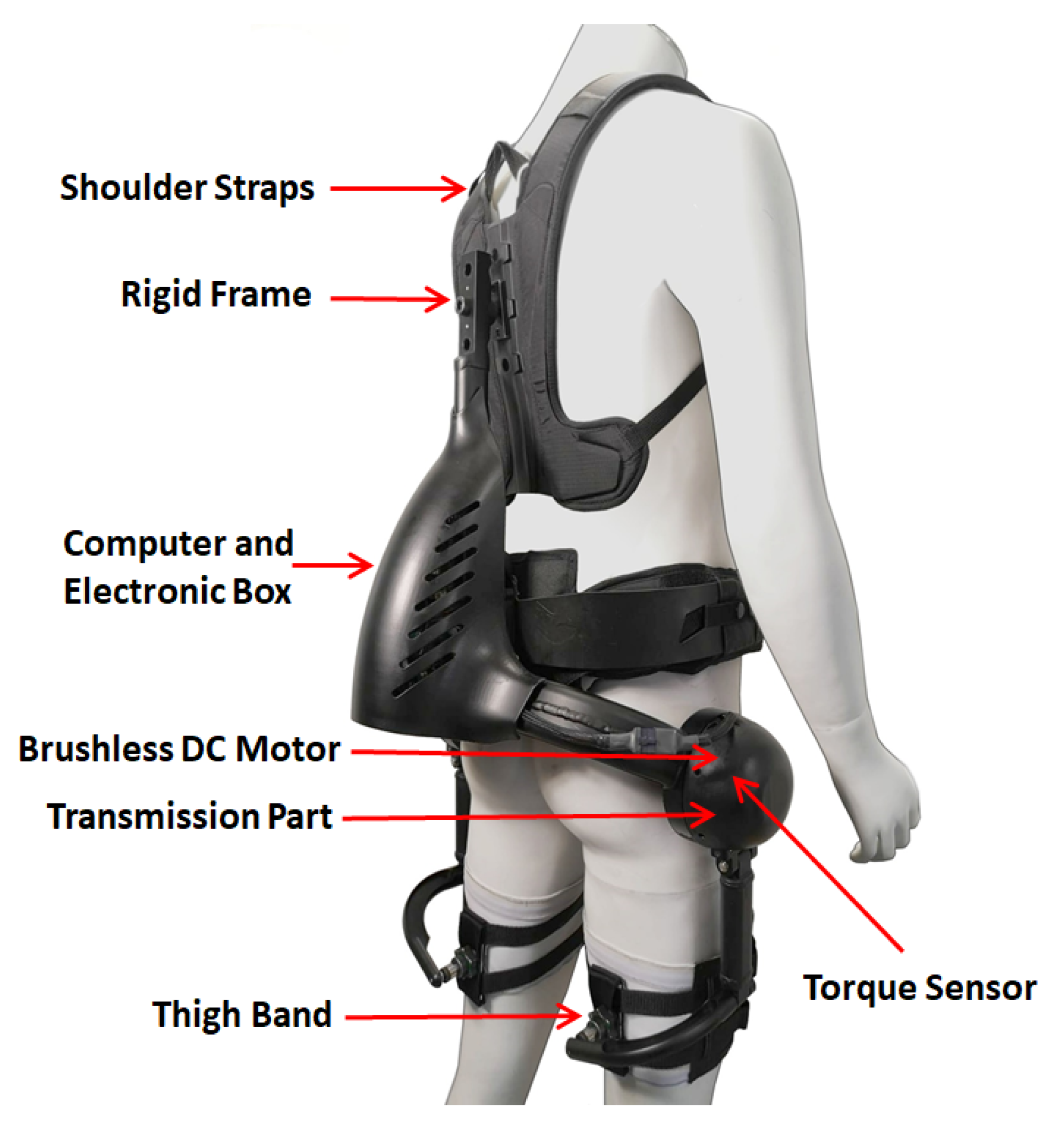
Considerable research effort has recently been devoted to the development of adequate models and control approaches for wearable robots such as exoskeletons [1]. Generally, an exoskeleton is worn by an operator to provide support and protection from physical activities by generating proper assistive force(s) and torque(s) [2]. Additionally, exoskeletons might be profitably used in such non-industrial areas such as military, medicine and rehabilitation [3]. For military applications, the exoskeletons are designed to enhance the travel abilities and loading capabilities of soldiers; for industrial purposes, the exoskeletons are used to augment an operator’s load-handling potential and avoid and even reduce the occurrence of musculoskeletal damages; in rehabilitation, exoskeletons improve the lost functions and the quality of life of patients with serious disabilities, motor cognitive restrictions [4]. An example of a back-support exoskeleton is illustrated in Figure 1.
Due to the direct interface between the operator and the physical structure there are a number of features in exoskeleton design that are not common, or not so critical, in the design of industrial robots. From the mechanical point of view, motion ranges, safety, user comfort, low inertia and adaptability should be taken into account [5]. On the other hand, controllability, responsiveness, flexible and smooth motion generation should be considered in exoskeleton control schemes [6].
With the intention of applying control schemes to exoskeletons and improving the system performance, a comprehensive dynamic model to represent the behaviour of this robotic platform is needed [7]. Simple dynamic models for exoskeleton robotic platforms such as the biomechanical model in 2D dimensional space [8], the Lagrangian dynamics model, specialized with a serial rigid links chain [9] and the mathematical model based on user’s movements [10] have been presented so far. Basically, precise dynamic model of the robotic platform represents the system behavior more accurately, which results in more appropriate and desirable control performance [11]. In addition, while achieving model accuracy for complex systems, the order of the system increases which results in complicated computations [12]. Modeling of complex systems such as exoskeletons through bond graphs requires fewer mathematical computations and is more adjustable and adaptable with respect to classical conventional dynamic modeling approaches. In this modeling approach, the dynamic systems are exhibited graphically, subsystems interconnected through bonds based on the flow of power in the system. This makes bond graph modeling an appropriate approach for modeling multidisciplinary dynamic systems [13].
On the other hand, one of the main issues for developing exoskeleton systems is the lack of appropriate measuring devices and methods for the direct measurement of all the system states. This issue can limit the use of some control techniques such as model-based controls [14] in terms of the state feedback [15] since model-based controls assume that the system dynamic is known [16]. More recently, Yang, et al. in [17] proposed a novel compliant upper-body exoskeleton platform to reduce spine loading across multiple vertebral joints. Although their robotic control system demonstrates a good robust behaviour, the tracking error is still high due to lack of information from the interaction forces and torques between the human body and exoskeleton. In the literature, several methods have been proposed to measure and estimate the human-robot interaction force/torque in exoskeleton applications. Choi in [18] developed and proposed a compact force sensor system for an exoskeleton platform to measure interaction force/torque. However, using force/torque sensors are generally expensive and cause an increase in the device weight and complexity. Some proposed methods rely on commanded actuation torques (motor currents) to estimate the interaction force/torque such as the work presented in [19]. Distinguishing the damping and elasticity effects of system components for identifying system dynamics is the main problem of these methods. Furthermore, employing EMG sensors to detect the biological signals from muscle activities to estimate interaction force/torque is another popular approach among researchers [20,21]. Nevertheless, EMG sensors are highly sensitive to to changes in skin conductivity skin conductivity, mounting and positioning, muscle fatigue and interactions between muscles. Using inverse dynamics [22], requiring high computational cost, is another method to estimate interaction force/torque. On this basis, the synthesis of a Kalman filter observer for a back-support exoskeleton for estimating interaction force/torque has been proposed and developed as one of the aims of this paper.
In this paper, a dynamic model, employing the bond graph modeling method, rather than the more conventional block diagram approach has been developed, presented and used to better analyze the behavior of the system. In other words, one can easily find out and analyze the effects of elements and variables on the dynamics of an industrial back-support exoskeleton platform. The bond graph modeling technique brings benefits in comparison with the other classical modeling techniques [23]:
- Providing a visual representation of main properties of the system by separating the system formation from dynamic modeling equations;
- Monitoring the coherence and consistency of the topological structure of the dynamic system;
- Providing a hierarchical dynamic model of the system.
Additionally, the synthesis of a Kalman filter observer for a back-support exoskeleton, besides bond graph modeling, is discussed and developed in this work. Kalman filters are usually very sensitive to the modeling errors. However, they can work well in closed-loop system schemes which provide good stability and performance despite large errors in the estimated values. The proposed Kalman observer needs only the measurement of the angular velocity of the electrical motor and the instant value of the torque signal from the output of the transmission section. Hence, the use of other sensors such as strain bridges or accelerometers are not required. The performance of the Kalman state observer has been examined in the simulation an experimental tests of a lifting task scenario by using a linear quadratic regulator (LQR) controller [24] with double integral action. The work, proposed and discussed in this paper, features a high level of originality, rather than the more conventional block diagram approach has been developed, presented and used to better analyze the behavior of the system.
The present paper aims to develop a bond graph model for industrial back-support exoskeletons as an alliterative to classical dynamic modeling methods to describe dynamic behaviors of the system. Furthermore, a general approach for designing a functional Kalman filter observer by means of a linear dynamic model for industrial back-support exoskeletons has been proposed. This formation overcomes the difficulties caused by geometric and technical structural constraints in of back-support exoskeleton dynamic models.
This paper is organized as follows: first, in Section 2, the dynamic model of a back-support exoskeleton is described in terms of block diagram and bond graph modeling. In Section 3, the synthesis of the Kalman State observer is given. The system identification procedure based on the experimental tests is discussed in Section 4. The performance analyses of both the bond graph model and Kalman state observer is discussed in Section 5. Finally, in Section 6, conclusions are drawn.
2. Dynamic Model
In this section, the dynamic model of an industrial back-support exoskeleton with respect to the block diagram and bond graph modeling approach is explained. Theoretically, wearing an exoskeleton results in interaction forces between the user’s body and the robotic structure. These interaction forces can be formulated and modeled through the linear mass-spring-damper system [25]. In this modeling approach, the masses reproduce the inertia properties of different body segments which includes hard and soft tissues. The biomechanical properties of the other segments comprising bones, muscles, tendons, and ligaments are represented by springs and dampers.
2.1. Block Diagram Model
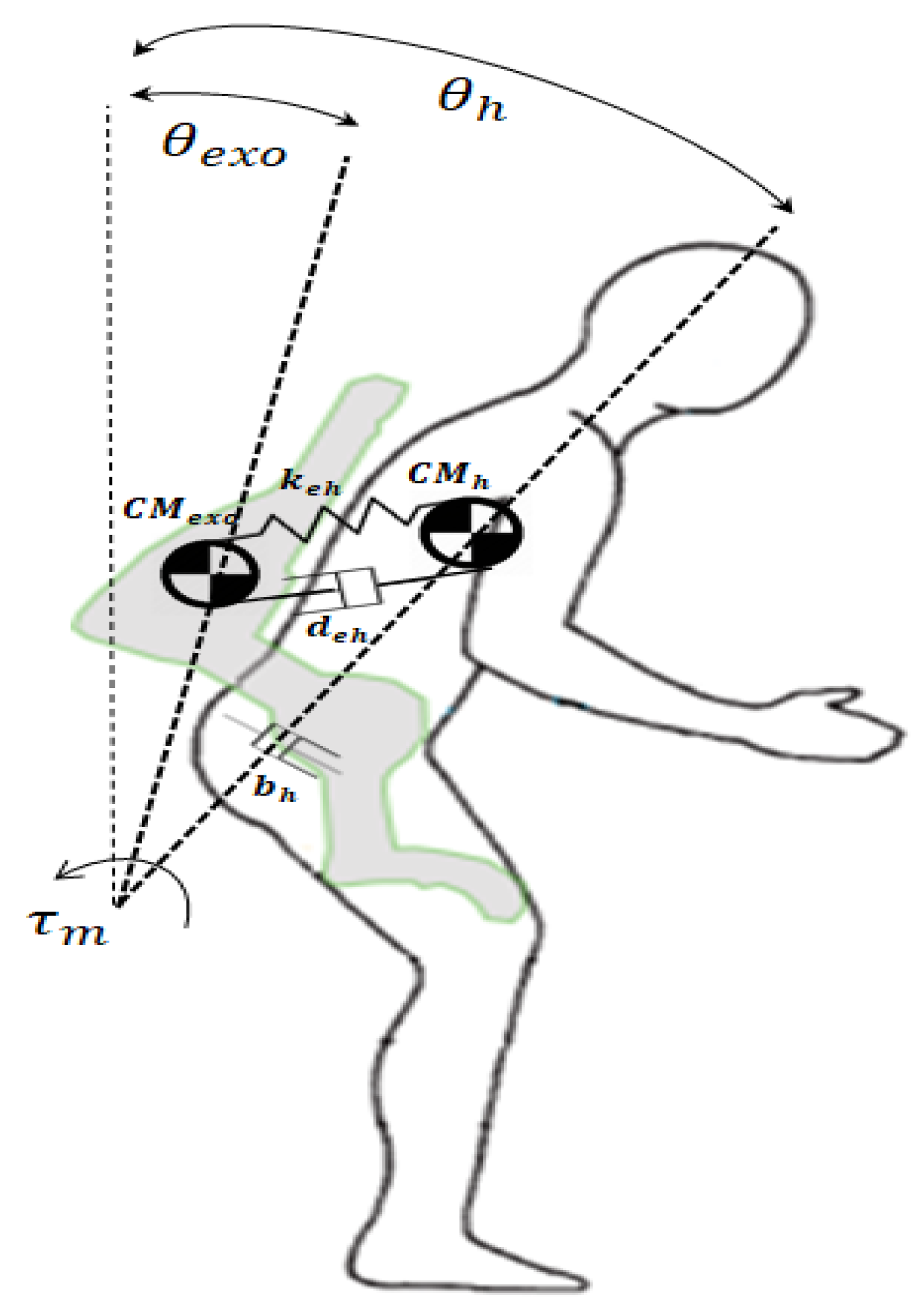
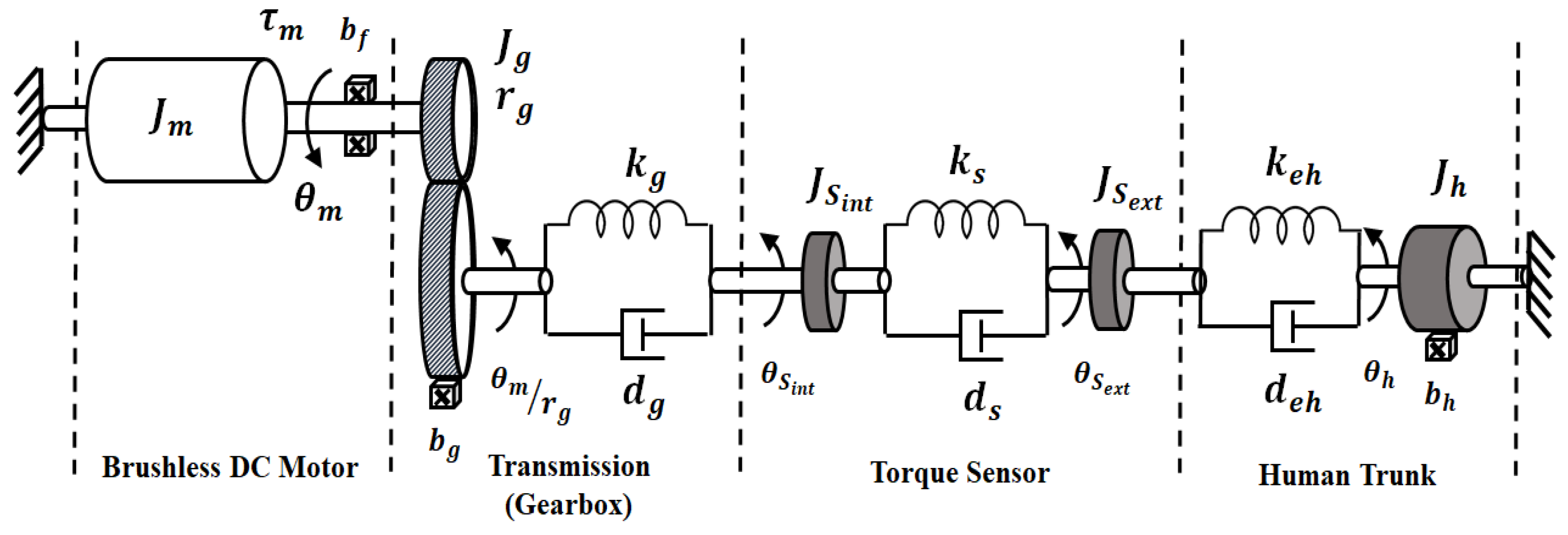
To formulate the the movement of the industrial back-support exoskeleton worn by the operator, a corresponding linear biomechanical model is shown in Figure 2. For the sake of simplicity, a graphical representation of the dynamic model of an industrial back-support exoskeleton is illustrated in Figure 3. The dynamic model comprises a brushless DC motor coupled through the rotor shaft to a gearbox transmission, a torque sensor and a the biomechanical model of the human trunk. Consequently, the dynamic model of the system can be formulated mathematically as:
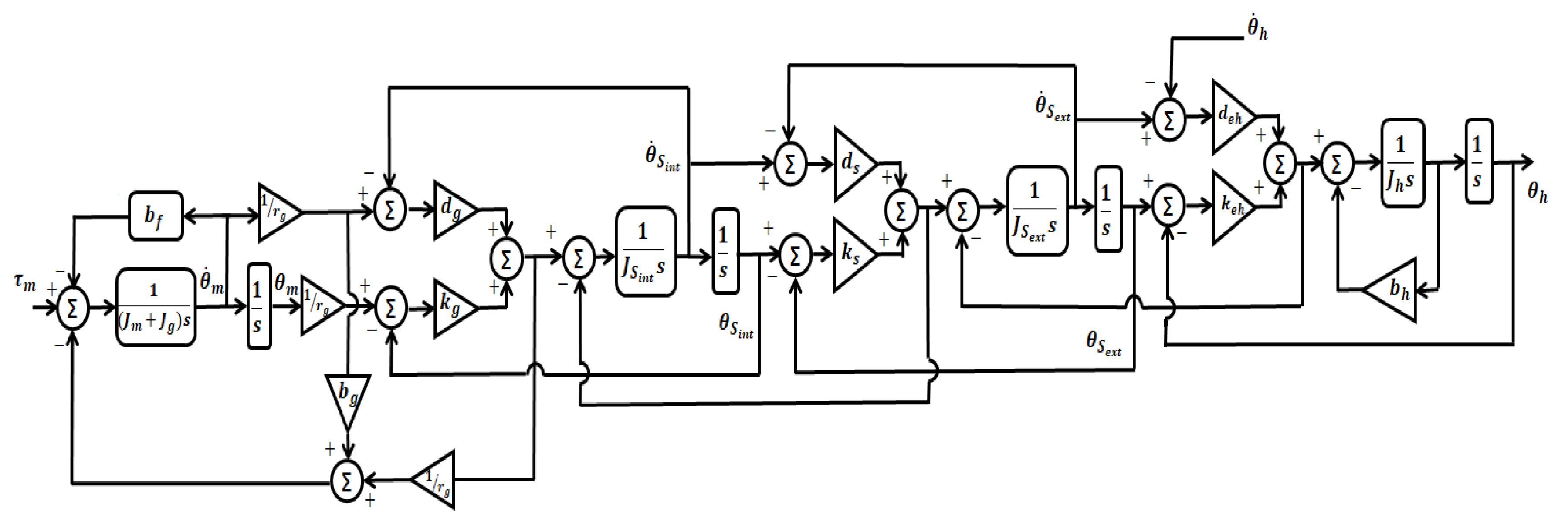
The parameters and variables of Equation (1) are defined in Table 1. By considering the human trunk velocity ( ) and motor torque () as the system inputs, the block diagram corresponding to the dynamic model of the industrial exoskeleton system can be depicted in Figure 4. This block diagram aims to reflect the constitution of the mathematical model. The codes for modeling the dynamic system, developed in the MATLAB environment, are given in Supplementary Materials.
2.2. Bond Graph Model
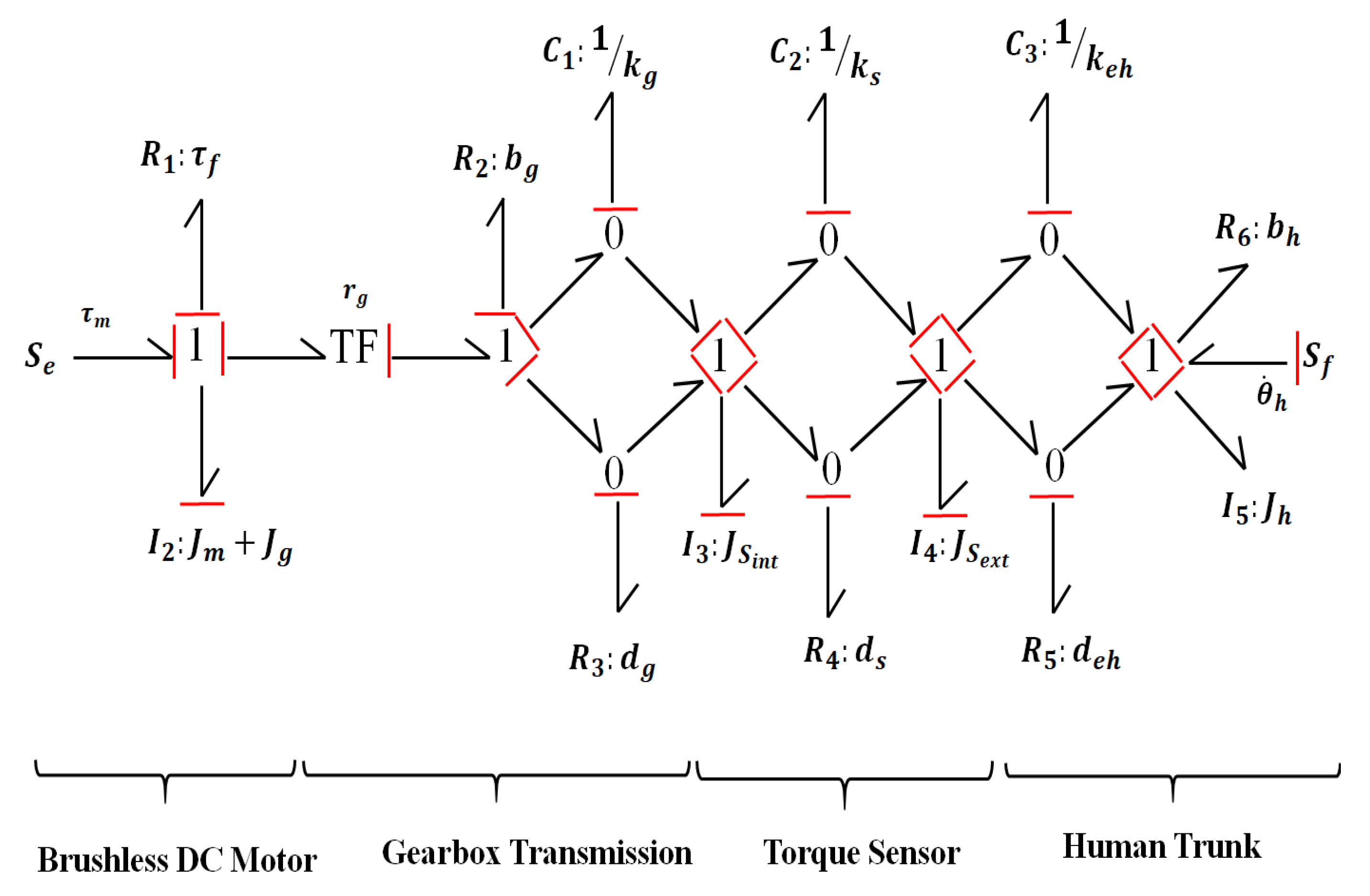
The bond graph modeling approach is a graphical technique to model and analyze the dynamics of physical dynamic systems from different domains to in a united style. In bond graph modeling approach, the ports of components are connected by bonds that specify the transfer of energy between dynamic system components. These components are described through their energetic behavior. In fact, they can either store or dissipate, supply or absorb, and transform energy reversibly or irreversibly [26]. More information and details about bond graph methodology are given in [27].
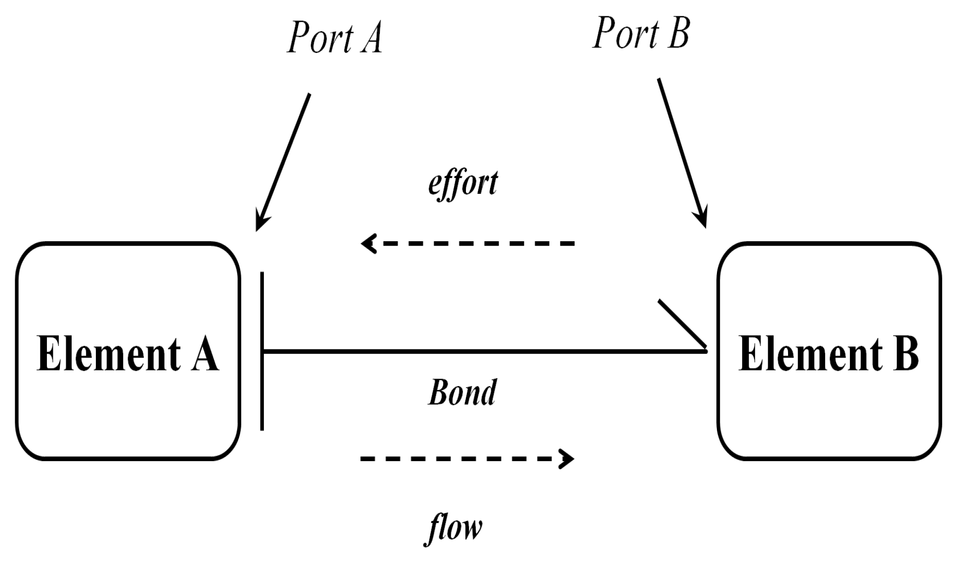
Bond graphs causality is a notation format that indicates which side of a bond determines the instantaneous effort and which determines the instantaneous flow. From the graphical point of view, the causality is shown by putting a vertical line close to the element which dominates the flow as illustrated in Figure 5. In dynamic equation formulations that describe the system, causality determines the dependency of variables which correspond to each dynamic modeling element. Consequently, a bond graph can present from different fields and domains in a unified way. Table 2 reports the effort and flow variables of different energy domains.
Based on the block diagram modeling descriptions in the earlier section, the bond graph of the exoskeleton framework can be shown in Figure 6. As can be seen from Figure 2, the exoskeleton robotic platform includes four main parts: brushless DC motor, gearbox transmission, torque sensor and human trunk. Consequently, corresponds to the output torque () of the brushless DC motor in Figure 6. The output torque of the brushless DC motor () drives the motor’s shaft with an inertia of as well as the gearbox transmission with input angular inertia of and it also overcomes the mechanical friction :. Because these elements are driven with the same velocity, the first (from the left to right) is a 1-type junction. In this work, the shaft of the brushless DC motor is assumed to be stiff.
The gearbox transmission is modeled as transformer () and its ratio number is represented as the transformer modulus (). The transformed velocity by the gearbox transmission which is effected by the gearbox friction () is given by the 1-type junction right to the element.
The speed difference between the gearbox transmission and the internal ring of the torque sensor inertia (:) drives the gearbox stiffness (:) and gearbox damping parameter (:) through a 0-type junction. The 0-type junctions generate the difference of speed maintaining a constant effort, while the second and third 1-type junction (from left to right) feed the speed differences to both : and : and splits the effort between both elements. In a similar way, the speed difference between the internal and external ring of the torque sensor (:) drives the torque sensor stiffness (:) and damping (:) toward a 0-type junction. As much as the torque acts on the external ring of the torque sensor, the corresponding effort is applied to : via an 1-type junction.
Regarding to the block diagram model of the system described in Figure 3, the human trunk contains the equivalent damping (:) and stiffness (:) between the trunk and exoskeleton and also human trunk inertia (:) and damping (:). Furthermore, the trunk velocity () is considered to be a system input. : and : have the same velocity (), while : and : are fed by the difference in the speed between : and :. Therefore, the human trunk inertia and damping are connected to the flow source (trunk velocity) through a 1-junction (5th from left to right).
3. Kalman Filter Observer Design
Basically, a state observer is a system that models a real dynamic system in order to provide an estimation of its internal state variables, given measurements of the input and output of the real dynamic system [28]. In our application, there is no direct measurement for the torque on the human body which is defined as the ratio of the applied torque to the deformation of the trunk muscles. Hence, there is a need for the state observer to obtain an estimation of the torque on the human body. In this section, the design of a Kalman state estimator [29] for a back-support exoskeleton has been explained. The first step to implement the Kalman state observer in our application is to take the state vector into account as:
Equation (1) can be reorganized and expressed in the form of a matrix representation (Equation (3)). Based on this, by taking process and measurement noises into the formulation, a more compact form of Equation (3) can be expressed in the form of state-space equations as follows:
where includes the first six states of and is equal to . comprising the first six rows and columns of A, containing the first six rows of the last column of A , consisting the first six rows of , including the first six rows of and and is equal to 1.
The measuring output and consists of the measured signal from the brushless DC motor velocity and the signal from the torque sensor respectively by setting:
A sufficient condition for designing a Kalman observer is is satisfying the observability condition of the system. On this basis and by considering and , it can be proved that the pair () fulfils the observability requirements for existence of an asymptotically stable Kalman observer. Additionally, the torque on the human body that should be estimated in our system is presented by and can be formulated as a system output:
in which
the observer model can be expressed by the following system of equations:
where and is asymptotically stable. L is Kalman gain and is chosen to minimize the mean square error between the estimated and the actual state variables. It can be proven that , where P is symmetric and a positive semi-definite solution of Riccati equation.
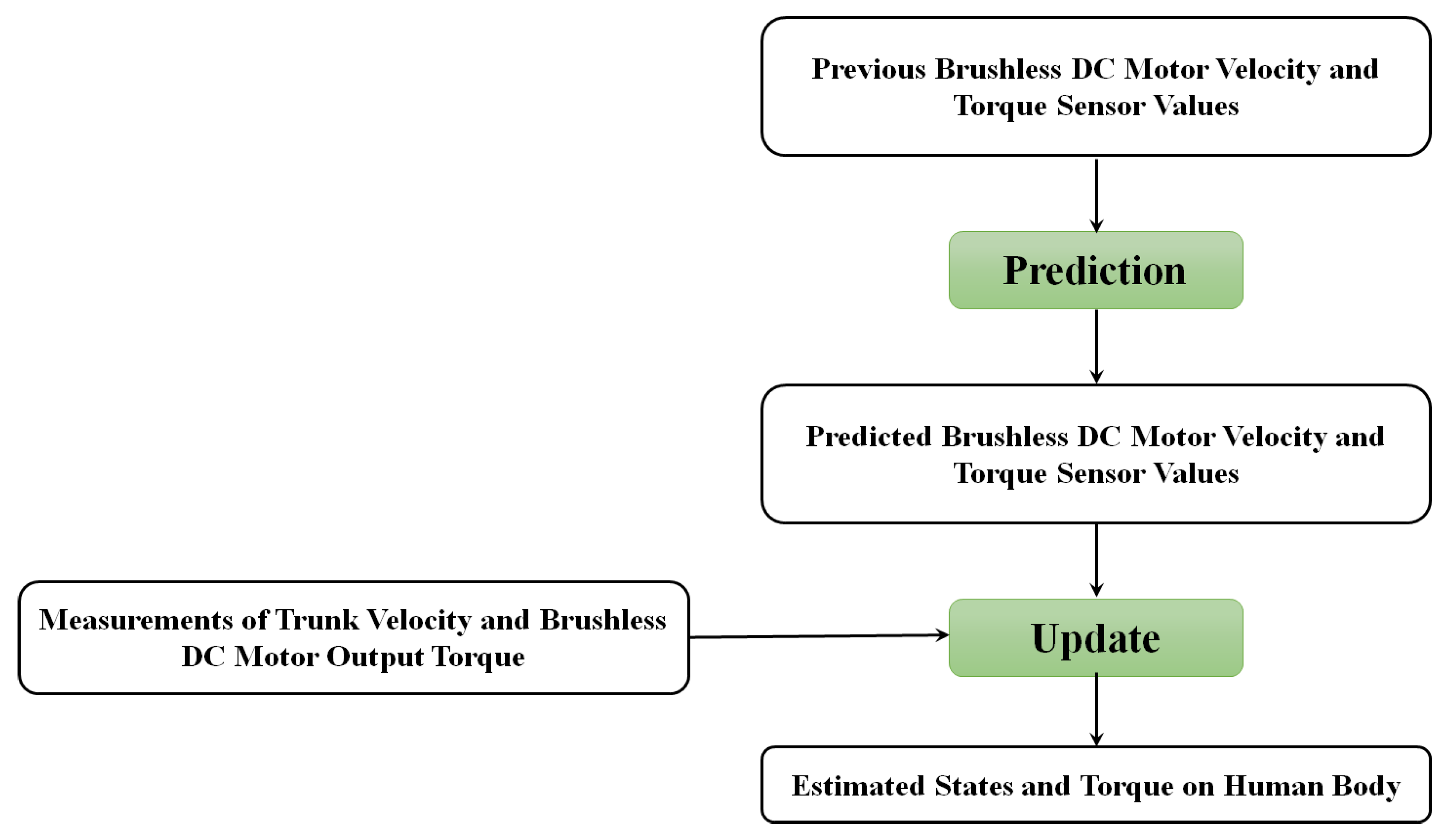
where and are the process and measurement noise covariance matrices. Additionally, represents estimated states while the estimated output is denoted by in Equation (7). The flowchart in Figure 7 shows the overall algorithm for the Kalman filter developed in this work.
4. System Identification
Friction and damping parameters have a fundamental role in the system dynamic and characterizing these parameters improves the model accuracy.. The value of was estimated from the experimental tests from the work in [7] using the same actuator and it is given by .
Some system parameters can be identified from components data-sheets provided by manufacturers; however, the information related to some parameters such as and are not reported anywhere. Hence, the experimental setup used for identification of and (shown in Figure 8) developed. This experimental setup comprises the same components used in our exoskeleton. In this setup, an inertia of is attached to the system in place of the human inertia (). Therefore in the model used for the identification test . The information of main components is reported in Table 3.
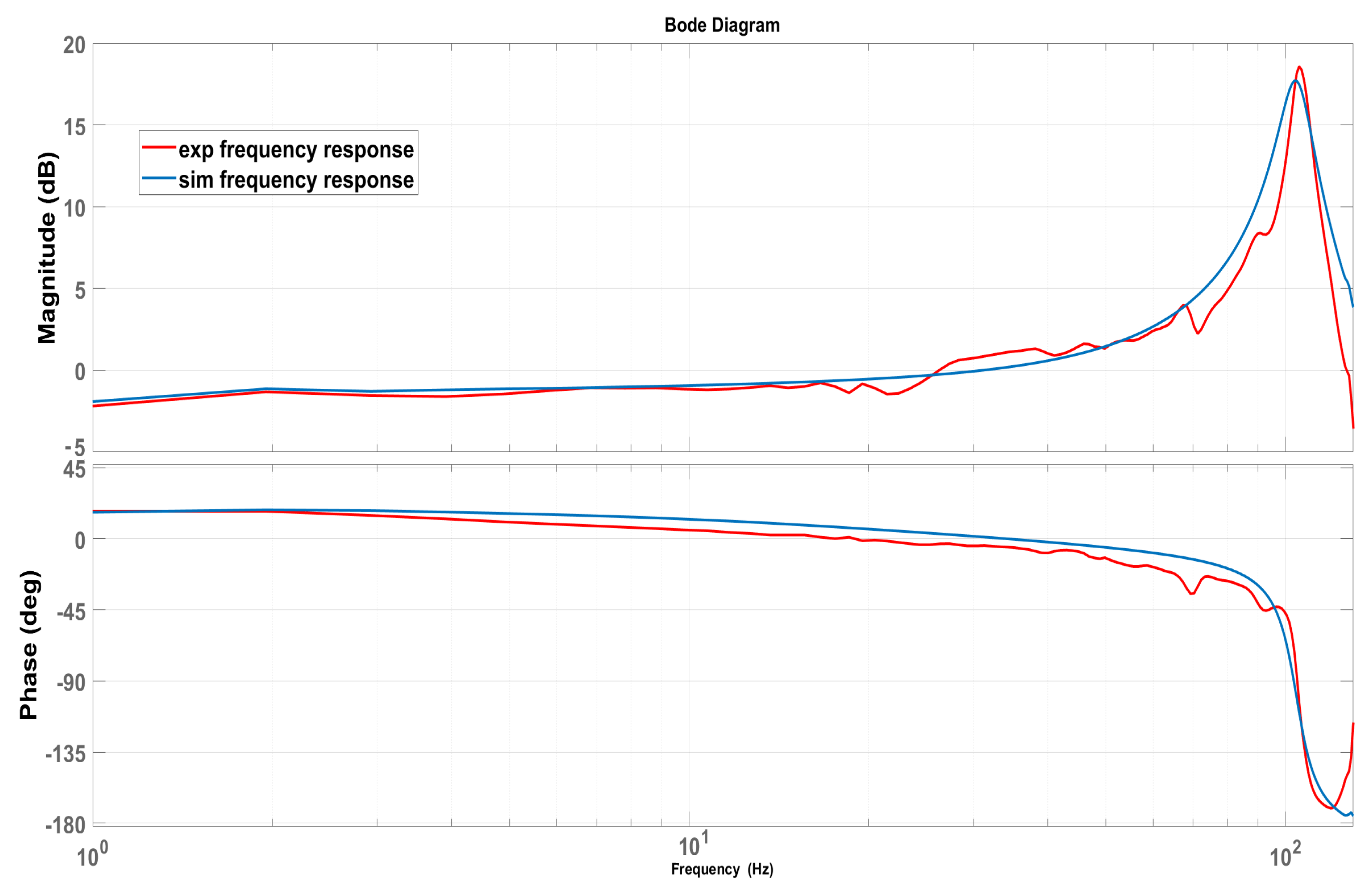
To identify the aforementioned unknown system parameters, we compare an experimental open-loop frequency sweep with the dynamic model presented in Section 2. To implement the experimental test, a current chirp reference signal with an amplitude of , which is equivalent to a torque with the amplitude of and the starting frequency () of and the final frequency () of 130 , was applied to the brushless DC motor. The bode plots extracted from the collected experimental data are shown in Figure 9. Correspondingly, the input data is the torque produced by the motor and the output is the torque signal measured by the torque sensor. By setting and a very high accuracy mathematical model corresponding to the experimental data can be obtained as is shown in Figure 9.
To obtain a more reliable dynamic model from the system, noise effects have been taken into consideration on system inputs (process) and outputs (measurements). In this work, and represent noise parameters on the motor torque input () and human velocity input () respectively. On the other hand, noise parameters on motor encoder and torque sensor signals are given by and respectively. The range used for these noise parameters are chosen based on the robot components as: , , and .
In addition, it should be mentioned that the values for and are extracted and estimated for a person with a weight of 75 and a height of as 1125 and respectively based on the work presented in [30]. Furthermore, the friction torque between the motor and gearbox transmission (), the damping coefficient between the human trunk and robotic platform (exoskeleton) () and torque sensor damping () are neglected as their values are so small with respect to those associated with the motor/gearbox and they can easily be compensated.
5. Simulation Results
5.1. Comparison between Block Diagram and Bond Graph Models
The simulation results from the block diagram and bond graph models are presented and discussed in this section. While the block diagram dynamic model of the exoskeleton robotic system is simulated via MATLAB software, the simulation of the bond graph modeling is carried out via 20-sim software [7]. The results from both simulation softwares are plotted with MATLAB.
The exoskeleton system, presented and discussed in previous sections, has been fed with an input torque of and a human trunk velocity of with a delay of . The simulations are carried out based on the torque sensed by the torque sensor as an effort variable in the terminology of the bond graph modeling and also the rotational velocity of the brushless DC motor shaft (gearbox transmission input velocity) is a flow variable in the terminology of the bond graph modeling. However, the simulation tests can be extended and implemented for all the system variables.
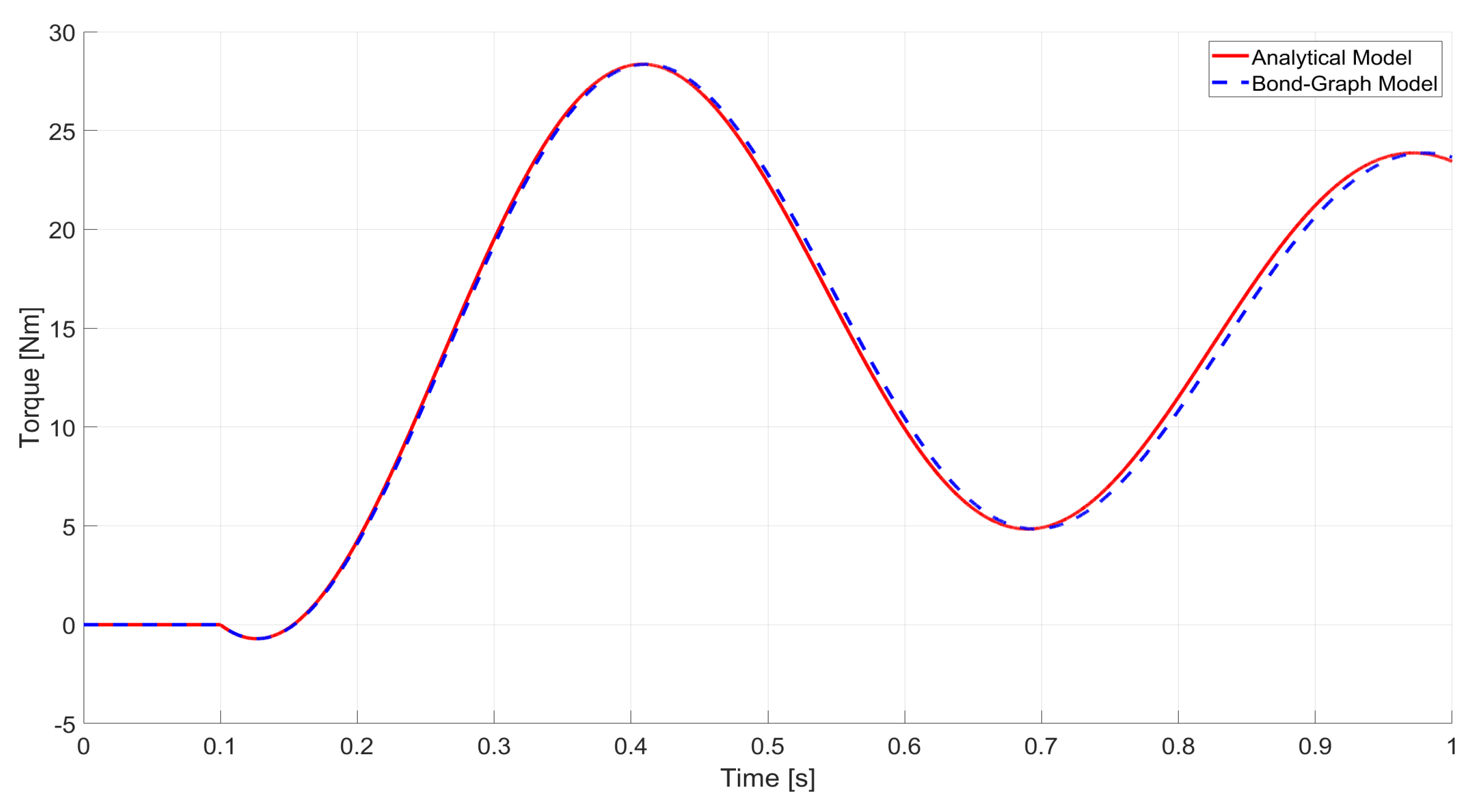
A comparison between the torque applied on the torque sensor through results from block diagram and bond graph models is demonstrated in Figure 10. From Figure 10, it can be inferred that the results from the bond graph model for the torque implemented on the torque sensor is very similar and close to that from the block diagram; however, the accuracy is slightly reduced as the robotic platform (human trunk) moves. The whole average error for the simulation test is around over 1 .
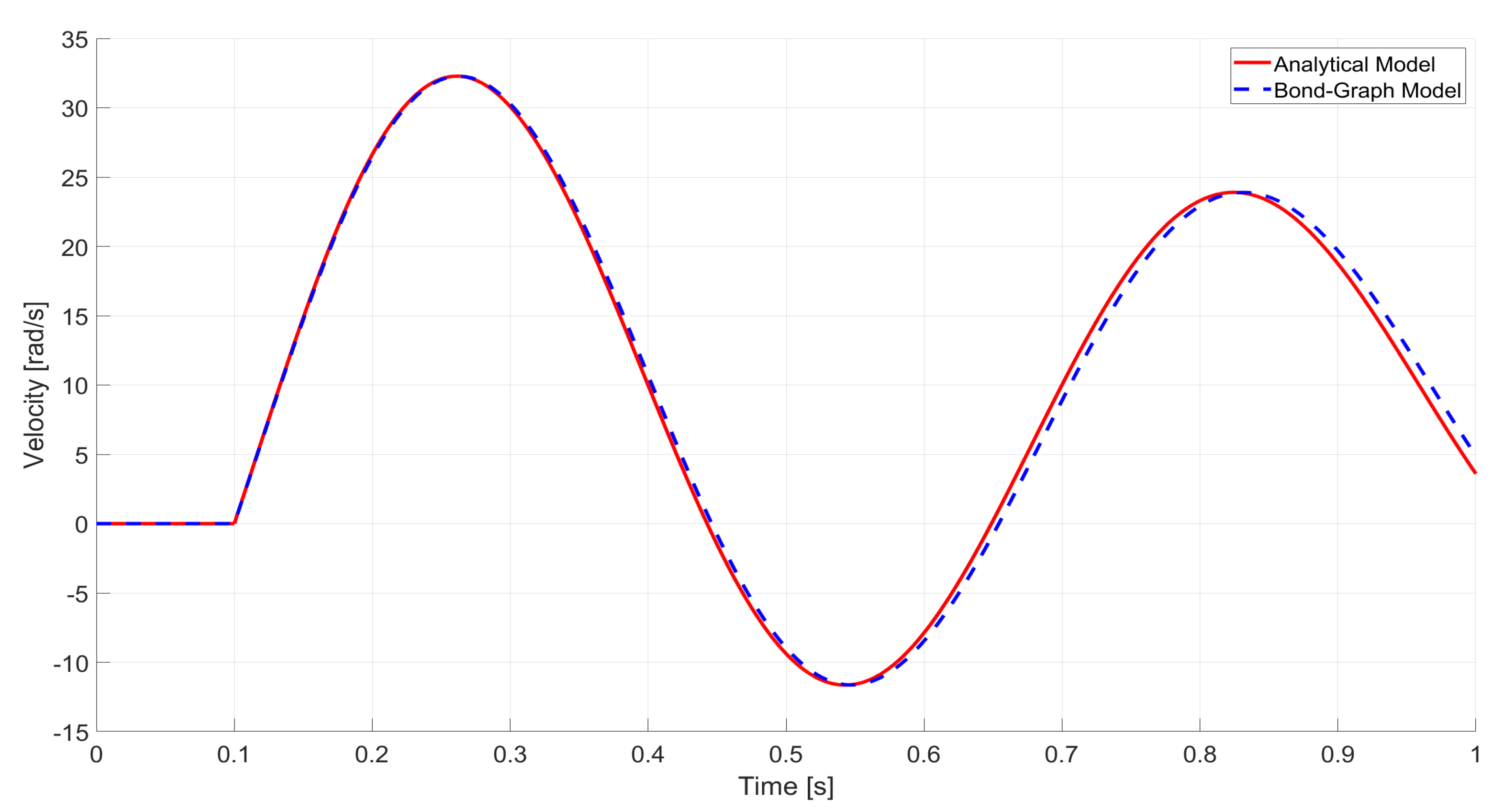
In addition, the difference between the rotational velocity of the brushless DC motor shaft through results from block diagram and bond graph models is shown in Figure 11. It can be concluded from Figure 11 that the two models are very close to each other and the overall average error is about during the first second. Accordingly, the error at the start of the movement slightly increases, but then it starts to approach zero over time.
Finally, an excellent agreement between the block diagram model developed in MATLAB and bond graph model developed in 20-sim can be inferred from both Figure 10 and Figure 11. It should be pointed out that using different numerical differential equation solvers with diverse configurations by MATALB and 20-sim is the main reason of the small errors between the simulation results [7].
5.2. Implementation of Kalman Filter Observer and Performance Analysis
The theory described in the forgoing sections means that both the dynamic model of the exoskeleton and Kalman observer can be implemented. The performance of the observer has been evaluated by comparing the values of the state variables computed by the simulator with the observer estimates on a test case using of a linear quadratic regulator (LQR) controller [31] with integral action. It is important to note that the synthesis and application of the Linear-Quadratic-Integral control is not described in detail as it is not pertinent to the Kalman observer design and performance assessment. All the simulation results have been executed by means of MATLAB.
The following state-space equations for the LQR controller with integrator action are taken into consideration:
where is the reference torque of the closed-loop control system and z is the auxiliary state corresponding to . Thereby, the optimal state-feedback control law is obtained in the form:
where represents the optimal feedback matrix gain, is the proportional matrix gain and indicates the integral gain. and are positive definite symmetric weighing matrices of the LQR cost function corresponding to the states from the Kalman observer and the human trunk velocity. It is worth mentioning that the states from the observer contains estimated values corresponding to and the estimated torque on the human body.
Varying and matrices cause changes in the location of the closed-loop poles which effects the performance of the system. While the large value of causes smaller control inputs and thereby larger values of the states, a faster convergence of the states could be obtained by larger elements of . The following consideration are used to achieve a proper feedback matrix:
where is equal to the difference between estimated and reference torque on the human body. To reject the ramp trajectories arising from the human trunk position during the constant human velocity, the LQR requires a double integrator. Hence, the following formulation is derived:
The LQR optimal control law of Equation (12) can be written as:
in which t represents the instantaneous time and is the variable of the integration associated with the time.
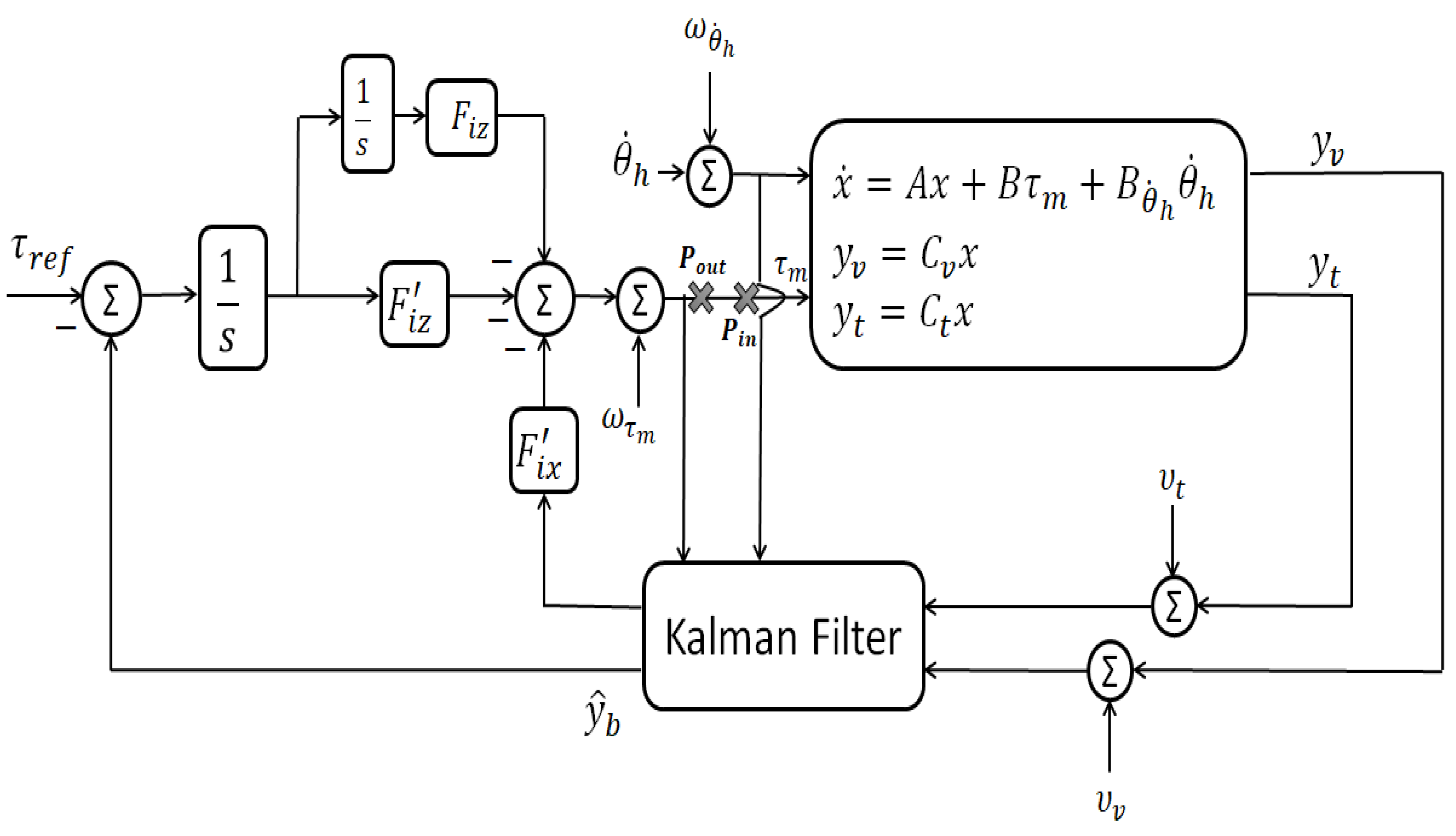
The controllability condition of the pair () is an adequate condition for the presence of a state feedback gain in a way that () be asymptotically stable. , the controller matrix, can be calculated by minimizing the quadratic performance index of the LQR controller for Equation (12). Figure 12 demonstrates the block diagram of the closed-loop control system. In Figure 12, is the gain related to the integrator term corresponding to the torque on the human trunk (last array of ) while the estimated torque on the human trunk is indicated by .
A simulation to evaluate the observer performance has been carried out. The main assumption of this simulation is that the exoskeleton works in assistive mode. That is, the human trunk moves with a constant velocity ( ) and an assistive torque is applied on the human body by the exoskeleton. This simulated scenario is archived by applying a step reference as the system input with an amplitude of 10 and a delay of for a time period of .
It is worth noting that the resulting and matrices and weighting matrices ( and ) associated with LQR related to Equation (12) are:
The final state feed-backs are extracted as follows:
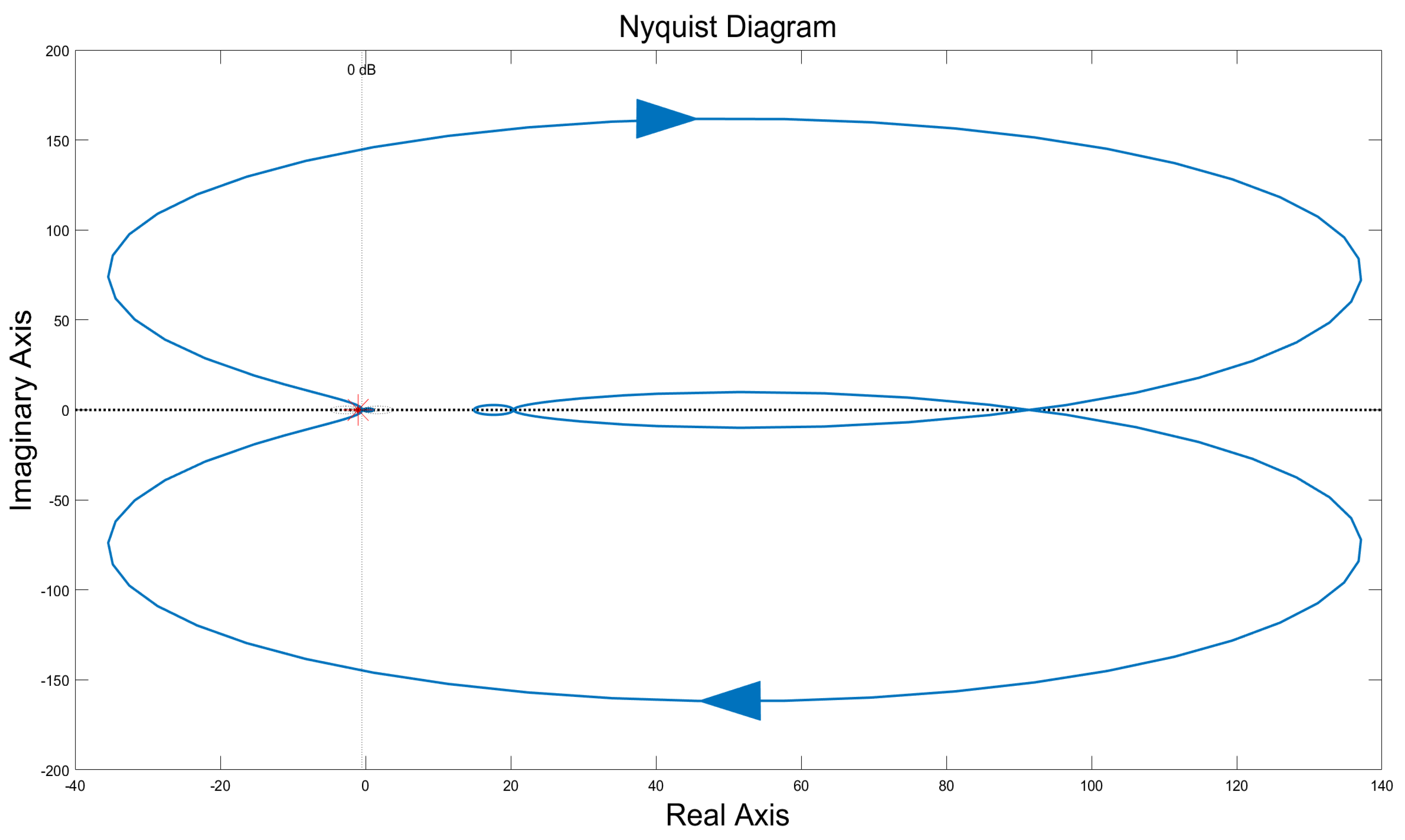
Essentially, controllers based on state feedback which are implemented through state observers can have disappointing properties regarding relative stability even when the state feedback and state observers demonstrate good and robust stability characteristics [32]. On this basis, stability margins have been evaluated by Nyquist plot (Figure 13 and Figure 14) of the loop gain, from the motor plant input (point in Figure 12) to the computed torque signal from the controller (point in Figure 12). We can see that the plot in Figure 13, does not encircle the critical point (), so the system is stable. Figure 14 shows the Nyquist plot in the neighborhood of the critical point. The nominal design has a minimum gain margin of approximately and minimum phase margin of about 59 with a delay margin of around which indicates that the minimum sampling frequency of the control unit should be almost 143 to guarantee stability.
The bode plot of the transfer function from the input disturbance (human trunk velocity) to the estimated torque on the human body is shown in Figure 15 to assess the disturbance rejection bandwidth. This determines how quickly the effects correlated with the human trunk motion decline to an acceptable level, for the exoskeleton platform. By considering the bandwidth as the first frequency in which the gain descends to below of its DC value, it can be inferred that the bandwidth for tracking disturbance (human trunk velocity) rejection is almost 52 ; nevertheless, it can be concluded that the human motion with the frequency range of 4∼6.2 has the most destructive effect on the estimated torque.
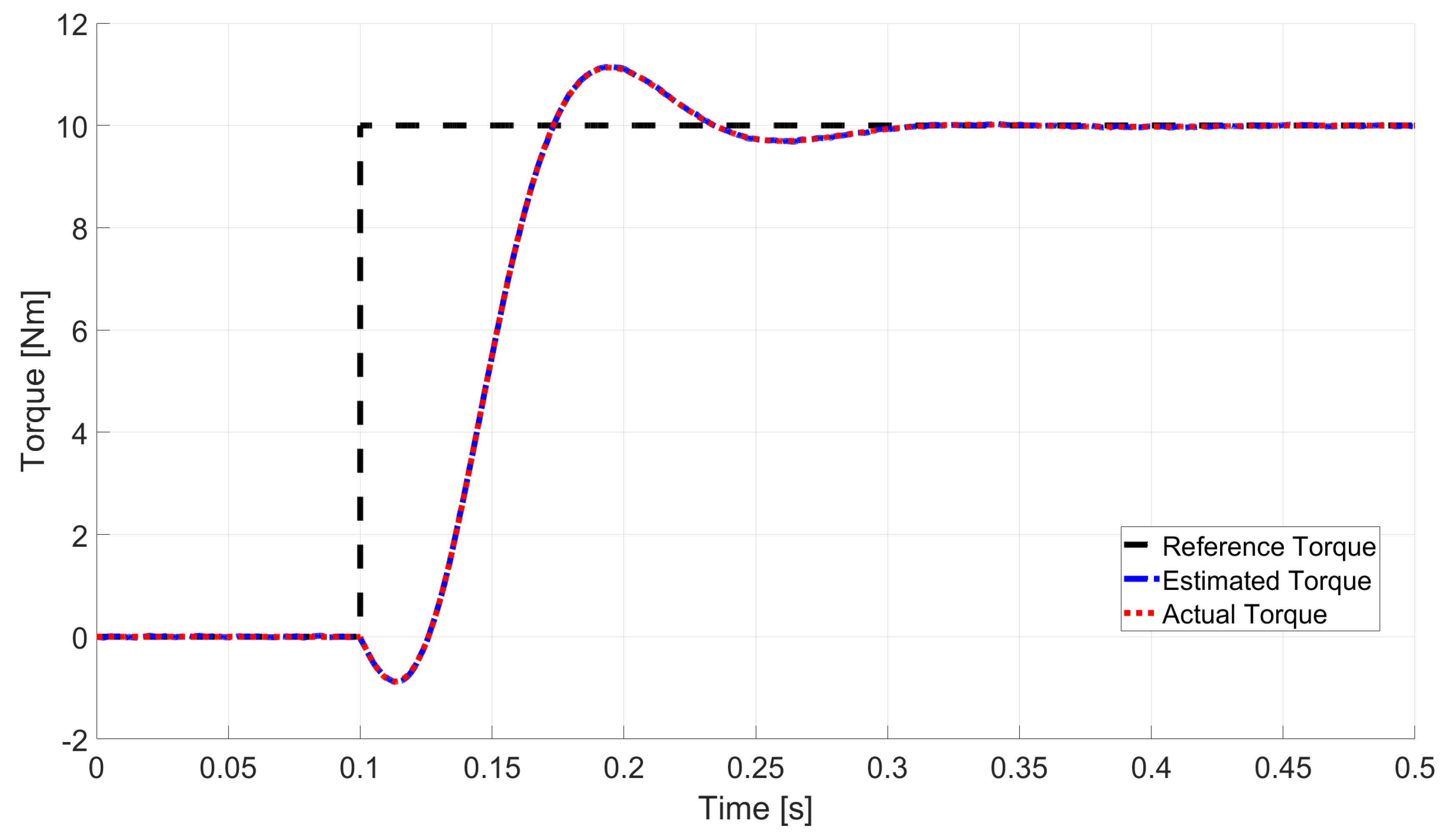
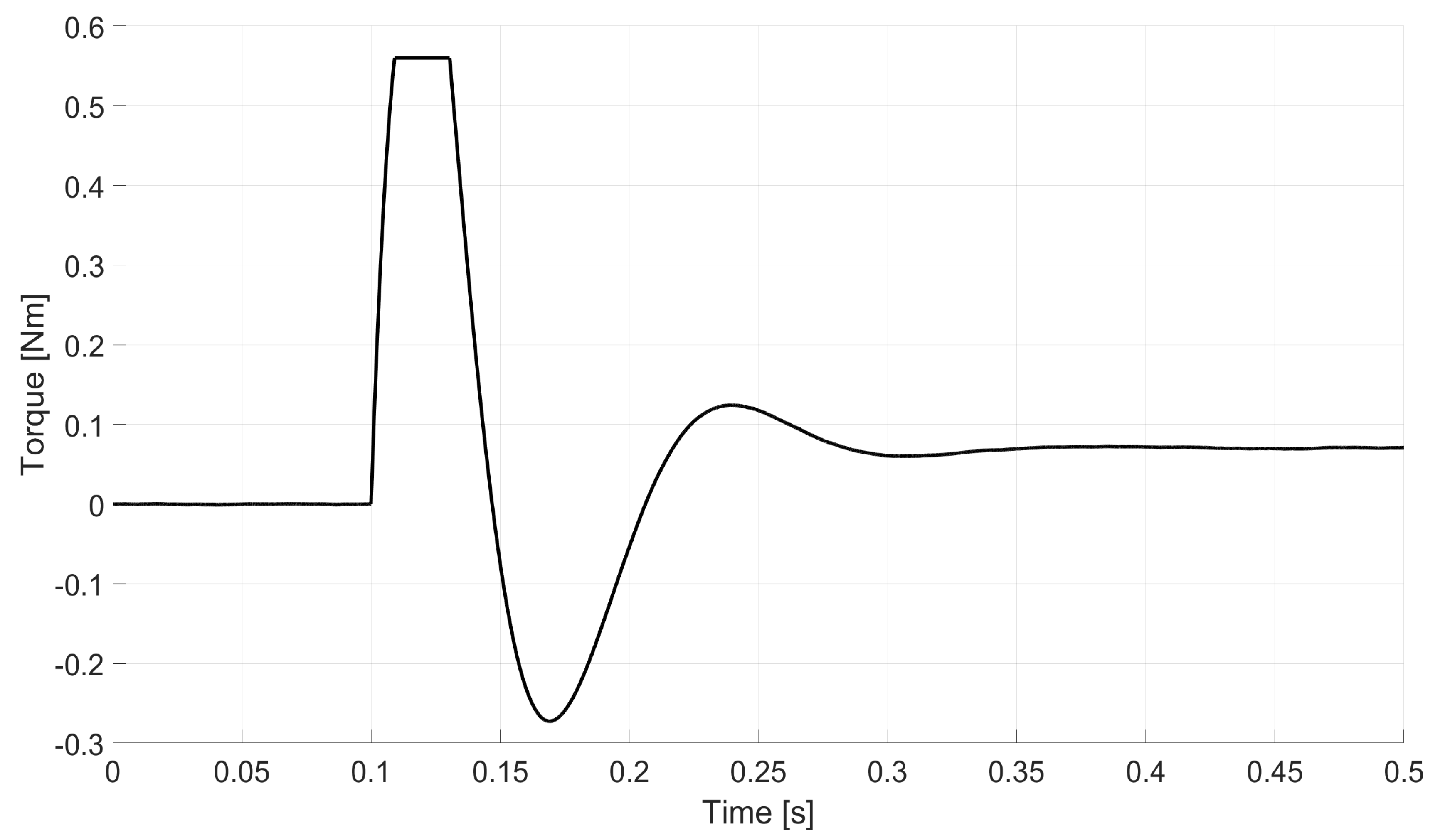
The first evidence of the observer’s effectiveness is reported in Figure 16 where a comparison is made between the step responses of the closed-loop control system using the proposed state observer and the linear dynamic model of the system. As it can be inferred from Figure 16, the step response of the observer and the linear model are very similar. Figure 17 shows the error on that is, the error between the linear model and the estimator in terms of torque on the human body. This is very small with the mean-squared error of about and approaches zero over time. Another interesting finding from Figure 16 is the undershoot at the beginning of the human motion. This occurs because of the phase delay between the human trunk motion velocity and the estimated torque (non-minimum phase system).
The DC motor velocity is shown by Figure 18 and Figure 19. While Figure 18 shows a comparison between the measured and estimated values of the motor velocity, the error between these values () over time is reported in Figure 19. Regarding these figures, the mean-squared error is around which implies a good agreement between the measured and estimated variables.
Furthermore, according to Figure 20, the overall torque produced by the brushless DC motor is in the defined torque limit range ( ).
6. Conclusions
In this work, the synthesis and design of a bond graph model and an effective Kalman filter observer for an industrial back-support exoskeleton platform are investigated and presented. Both the bond graph model and Kalman observer, presented in this work, can be extended and implemented on all types of active wearable robots.
After the development the dynamic equations of the robotic platform and extraction of the bond graph model and Kalman state observer of the system, the validation procedure is carried out. The bond graph model, corresponding to an industrial back-support exoskeleton, is validated to allow comparison comparison between the results from bond graph approach and those from the block diagram dynamic model according to the torque sensed by the torque sensor and the velocity of the rotational brushless DC motor shaft. It can be inferred that the responses of the two dynamic models lead to very similar trends, as the errors (the difference between the responses) are quite small. On the other hand, the proposed Kalman filter observer makes use of an analytical dynamic model and leads to the synthesis of an observer with a structure combining the features of an asymptotic Kalman estimator and a linear system. This structure overcomes the difficulties arising from measuring directly the human-robot interaction torque. The results of the observer, achieved from the simulation environment through a Linear-Quadratic-regulator (LQR) control with double integrator action and the full state feedback, illustrate an accurate estimation a very low estimation error. The availability of an effective and computationally efficient state observer represents an essential starting point for the synthesis and experimental validation of model-based control schemes based on state vector feedback.
The main challenge of the presented work is to derive a dynamic model for the human body. There is, of course, a relatively wide variation in the characteristics of the human body and current approaches and data are not yet adequate in these areas.
Future work will consider the experimental validation of both the proposed bond graph model and Kalman filter observer on a real-time hardware by imposing a bound to the frequency content of the simulated system dynamics.
Supplementary Materials
The following are available at https://0-www-mdpi-com.brum.beds.ac.uk/2411-9660/4/4/53/s1.
Author Contributions
Conceptualization, E.S.B.; writing—original draft preparation, E.S.B.; software, E.S.B. and J.O.; validation, E.S.B. and J.O.; methodology, E.S.B. and J.O.; writing—review and editing, E.S.B., J.O. and D.G.C.; supervision, J.O. and D.G.C. All authors have read and agreed to the published version of the manuscript.
Funding
This work has been funded by Italian Workers’ Compensation Authority (INAIL) for the development of wearable assistive exoskeletons and hosted by Istituto Italiano di Tecnologia (IIT).
Conflicts of Interest
The authors declare no conflict of interest.
Abbreviations
The following abbreviations are used in this manuscript:
| LQR | Linear Quadratic Regulator |
| DC | Direct Current |
References
- Barjuei, E.S.; Ardakani, M.M.G.; Caldwell, D.G.; Sanguineti, M.; Ortiz, J. Optimal Selection of Motors and Transmissions in Back-Support Exoskeleton Applications. IEEE Trans. Med. Robot. Bionics 2020, 2, 320–330. [Google Scholar] [CrossRef]
- Barjuei, E.S.; Ardakani, M.M.G.; Caldwell, D.G.; Sanguineti, M.; Ortiz, J. On the Optimal Selection of Motors and Transmissions for a Back-Support Exoskeleton. In Proceedings of the 2019 IEEE International Conference on Cyborg and Bionic Systems (CBS), Munich, Germany, 18–20 September 2019; pp. 42–47. [Google Scholar]
- Gopura, R.; Bandara, D.; Kiguchi, K.; Mann, G.K. Developments in hardware systems of active upper-limb exoskeleton robots: A review. Robot. Auton. Syst. 2016, 75, 203–220. [Google Scholar] [CrossRef]
- Guan, X.; Ji, L.; Wang, R. Development of Exoskeletons and Applications on Rehabilitation. In Proceedings of the MATEC Web of Conferences, Amsterdam, The Netherlands, 23–25 March 2016; EDP Sciences: Paris, France, 2016; Volume 40, p. 02004. [Google Scholar]
- Roveda, L.; Savani, L.; Arlati, S.; Dinon, T.; Legnani, G.; Tosatti, L.M. Design methodology of an active back-support exoskeleton with adaptable backbone-based kinematics. Int. J. Ind. Ergon. 2020, 79, 102991. [Google Scholar] [CrossRef]
- Crowell, H.P.; Park, J.H.; Haynes, C.A.; Neugebauer, J.M.; Boynton, A.C. Design, evaluation, and research challenges relevant to exoskeletons and exosuits: A 26-year perspective from the US Army Research Laboratory. IISE Trans. Occup. Ergon. Hum. Factors 2019, 7, 199–212. [Google Scholar] [CrossRef]
- Barjuei, E.S.; Toxiri, S.; Medrano-Cerda, G.A.; Caldwell, D.G.; Ortiz, J. Bond Graph Modeling of an Exoskeleton Actuator. In Proceedings of the 2018 10th Computer Science and Electronic Engineering (CEEC), Colchester, UK, 19–21 September 2018; pp. 101–106. [Google Scholar]
- Koopman, A.S.; Näf, M.; Baltrusch, S.J.; Kingma, I.; Rodriguez-Guerrero, C.; Babič, J.; de Looze, M.P.; van Dieën, J.H. Biomechanical evaluation of a new passive back support exoskeleton. J. Biomech. 2020, 109795. [Google Scholar] [CrossRef]
- Wang, H.; Ni, S.; Tian, Y. Modeling and control of 4-DOF powered upper limb exoskeleton. In Proceedings of the 2017 32nd Youth Academic Annual Conference of Chinese Association of Automation (YAC), Hefei, China, 19–21 May 2017; pp. 304–309. [Google Scholar]
- Zoss, A.B.; Kazerooni, H.; Chu, A. Biomechanical design of the Berkeley lower extremity exoskeleton (BLEEX). IEEE/ASME Trans. Mech. 2006, 11, 128–138. [Google Scholar] [CrossRef]
- Barjuei, E.S. Hybrid position/force control of a spatial compliant mechanism. Int. J. Automot. Mech. Eng. 2017, 14, 4531–4541. [Google Scholar] [CrossRef]
- Saeed, M.T.; Khaydarov, S.; Ashagre, B.L.; Zafar, M. Comprehensive Bond Graph Modeling and Optimal Control of an Anthropomorphic Mechatronic Prosthetic Hand. In Proceedings of the 2019 IEEE International Conference on Mechatronics and Automation (ICMA), Tianjin, China, 4–7 August 2019; pp. 2006–2011. [Google Scholar]
- Mukherjee, A.; Karmakar, R.; Samantaray, A.K. Bond Graph in Modeling, Simulation and Fault Identification; IK International: Delhi, India, 2006. [Google Scholar]
- Vantilt, J.; Tanghe, K.; Afschrift, M.; Bruijnes, A.K.; Junius, K.; Geeroms, J.; Aertbeliën, E.; De Groote, F.; Lefeber, D.; Jonkers, I.; et al. Model-based control for exoskeletons with series elastic actuators evaluated on sit-to-stand movements. J. Neuroeng. Rehabil. 2019, 16, 65. [Google Scholar] [CrossRef]
- Tran, D.T.; Jin, M.; Ahn, K.K. Nonlinear Extended State Observer Based on Output Feedback Control for a Manipulator with Time-Varying Output Constraints and External Disturbance. IEEE Access 2019, 7, 156860–156870. [Google Scholar] [CrossRef]
- Barjuei, E.S.; Ortiz, J. A comprehensive performance comparison of linear quadratic regulator (LQR) controller, model predictive controller (MPC), H∞ loop shaping and μ-synthesis on spatial compliant link-manipulators. Int. J. Dyn. Control 2020. [Google Scholar] [CrossRef]
- Yang, X.; Huang, T.H.; Hu, H.; Yu, S.; Zhang, S.; Zhou, X.; Carriero, A.; Yue, G.; Su, H. Spine-inspired continuum soft exoskeleton for stoop lifting assistance. IEEE Robot. Autom. Lett. 2019, 4, 4547–4554. [Google Scholar] [CrossRef] [Green Version]
- Choi, H.; Seo, K.; Hyung, S.; Shim, Y.; Lim, S.C. Compact hip-force sensor for a gait-assistance exoskeleton system. Sensors 2018, 18, 566. [Google Scholar] [CrossRef] [PubMed] [Green Version]
- Gupta, A.; O’Malley, M.; Patoglu, V.; Burgar, C. Design, Control and Performance of RiceWrist: A Force Feedback Wrist Exoskeleton for Rehabilitation and Training. Int. J. Robot. Res. 2008, 27, 233–251. [Google Scholar] [CrossRef]
- Lyu, M.; Chen, W.; Ding, X.; Wang, J.; Pei, Z.; Zhang, B. Development of an EMG-Controlled Knee Exoskeleton to Assist Home Rehabilitation in a Game Context. Front. Neurorobot. 2019, 13, 67. [Google Scholar] [CrossRef] [PubMed] [Green Version]
- Yang, C.; Zeng, C.; Liang, P.; Li, Z.; Li, R.; Su, C.Y. Interface design of a physical human–robot interaction system for human impedance adaptive skill transfer. IEEE Trans. Autom. Sci. Eng. 2017, 15, 329–340. [Google Scholar] [CrossRef]
- Deng, J.; Wang, P.; Li, M.; Guo, W.; Zha, F.; Wang, X. Structure design of active power-assist lower limb exoskeleton APAL robot. Adv. Mech. Eng. 2017, 9, 1687814017735791. [Google Scholar] [CrossRef]
- Borutzky, W. Bond Graph Modelling of Engineering Systems; Springer: Berlin, Germany, 2011; Volume 103. [Google Scholar]
- Abdolshah, S.; Barjuei, E.S. Linear quadratic optimal controller for cable-driven parallel robots. Front. Mech. Eng. 2015, 10, 344–351. [Google Scholar] [CrossRef]
- Nikooyan, A.A.; Zadpoor, A.A. Mass–spring–damper modelling of the human body to study running and hopping–an overview. Proc. Inst. Mech. Eng. Part H 2011, 225, 1121–1135. [Google Scholar] [CrossRef]
- Das, S. Mechatronic Modeling and Simulation Using Bond Graphs, 1st ed.; CRC Press, Inc.: Boca Raton, FL, USA, 2009. [Google Scholar]
- Karnopp, D.; Margolis, D.; Rosenberg, R. System Dynamics: Modeling and Simulation of Mechatronic Systems; A Wiley-Intersience Publication, Wiley: Hoboken, NJ, USA, 2000. [Google Scholar]
- Barjuei, E.; Gasparetto, A. Predictive Control of Spatial Flexible Mechanisms. Int. J. Mech. Control 2015, 16, 85–96. [Google Scholar]
- Andersson, L.E.; Imsland, L.; Brekke, E.F.; Scibilia, F. On Kalman filtering with linear state equality constraints. Automatica 2019, 101, 467–470. [Google Scholar] [CrossRef]
- Moreno Catalá, M.; Schroll, A.; Laube, G.; Arampatzis, A. Muscle strength and neuromuscular control in low-back pain: Elite athletes versus general population. Front. Neurosci. 2018, 12, 436. [Google Scholar] [CrossRef] [PubMed] [Green Version]
- Barjuei, E.S.; Boscariol, P.; Gasparetto, A.; Giovagnoni, M.; Vidoni, R. Control design for 3D flexible link mechanisms using linearized models. In Advances on Theory and Practice of Robots and Manipulators; Springer: Berlin, Germany, 2014; pp. 181–188. [Google Scholar]
- Medrano-Cerda, G.; Eldukhri, E.; Cetin, M. Balancing and attitude control of double and triple inverted pendulums. Trans. Inst. Meas. Control 1995, 17, 143–154. [Google Scholar] [CrossRef]
Figure 1.
Back-support exoskeleton main components.

Figure 2.
Schematic view of the sagittal plane of an back-support exoskeleton and its operator according to the mass-spring-damper model.
Figure 2.
Schematic view of the sagittal plane of an back-support exoskeleton and its operator according to the mass-spring-damper model.

Figure 3.
Graphical representation of an exoskeleton robotic system.

Figure 4.
Block diagram representation of the exoskeleton system.

Figure 5.
Common conventions of bond graph causality.

Figure 6.
Bond graph model of the exoskeleton system.

Figure 7.
The flowchart of the Kalman filter algorithm developed in this work.

Figure 8.
The experimental setup for characterizing system parameters.

Figure 9.
Bode plots associated with the open-loop torque response to the motor current input. Red dashes are collected experimental data, the black line is the response of the identified model.
Figure 9.
Bode plots associated with the open-loop torque response to the motor current input. Red dashes are collected experimental data, the black line is the response of the identified model.

Figure 10.
Comparison between the torque applied on the torque sensor from results for the block diagram and bond graph models.
Figure 10.
Comparison between the torque applied on the torque sensor from results for the block diagram and bond graph models.

Figure 11.
Comparison between the rotational velocity of the brushless DC motor shaft through results from block diagram and bond graph models.
Figure 11.
Comparison between the rotational velocity of the brushless DC motor shaft through results from block diagram and bond graph models.

Figure 12.
Block diagram of the closed-loop control system.

Figure 13.
Nyquist diagram of the open-loop system from the motor plant input to the computed torque signal from the controller: Overall Nyquist (Not Scaled).
Figure 13.
Nyquist diagram of the open-loop system from the motor plant input to the computed torque signal from the controller: Overall Nyquist (Not Scaled).

Figure 14.
Nyquist diagram of the open-loop system from the motor plant input to the computed torque signal from the controller: Nyquist in the neighborhood of the critical point ().
Figure 14.
Nyquist diagram of the open-loop system from the motor plant input to the computed torque signal from the controller: Nyquist in the neighborhood of the critical point ().

Figure 15.
Bode plots associated with the transfer function from the input disturbance to the estimated torque on the human body.
Figure 15.
Bode plots associated with the transfer function from the input disturbance to the estimated torque on the human body.

Figure 16.
Step response of the system for estimated and actual torque on the human body.

Figure 17.
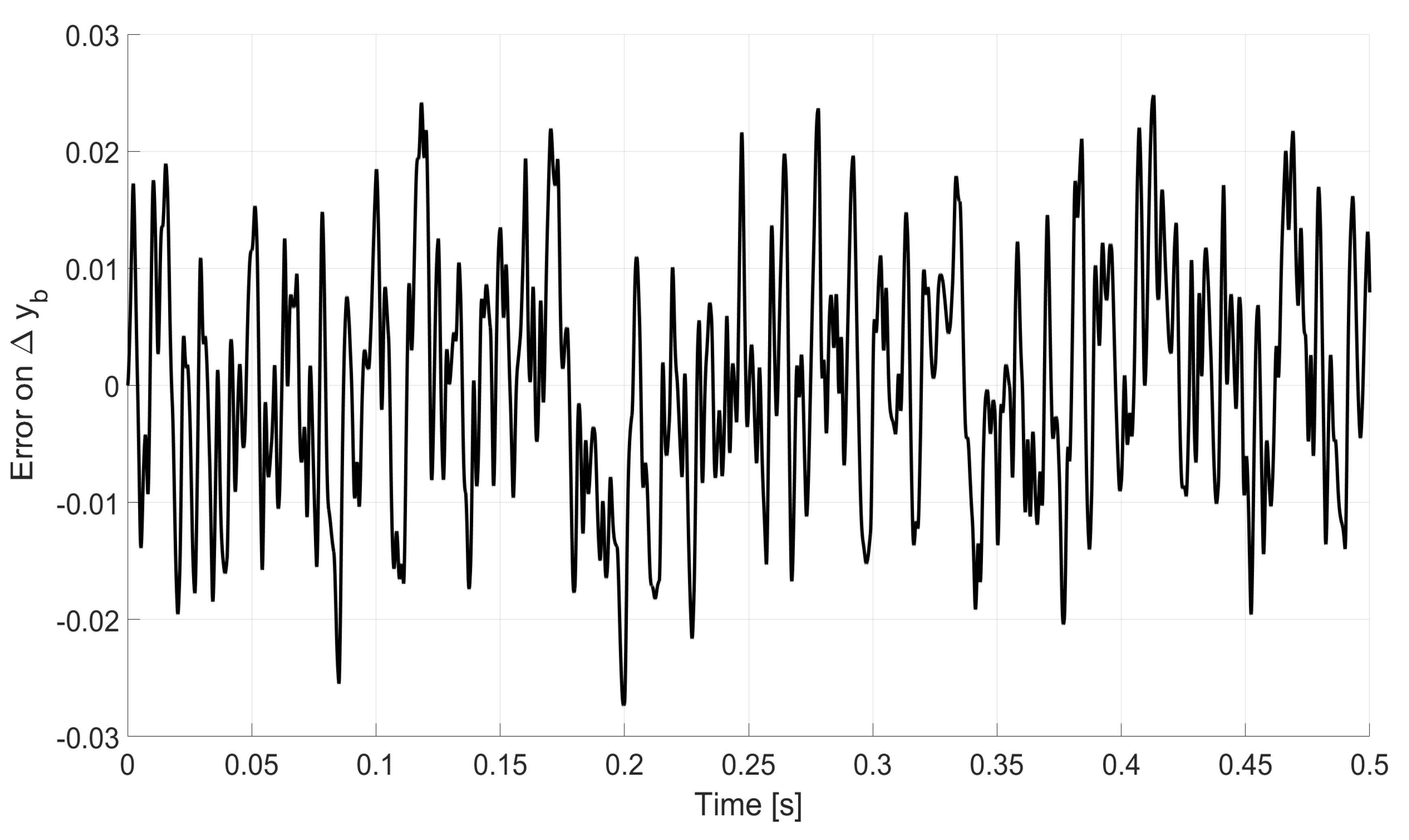
Error between the actual and the estimated values of the torque on the human body.

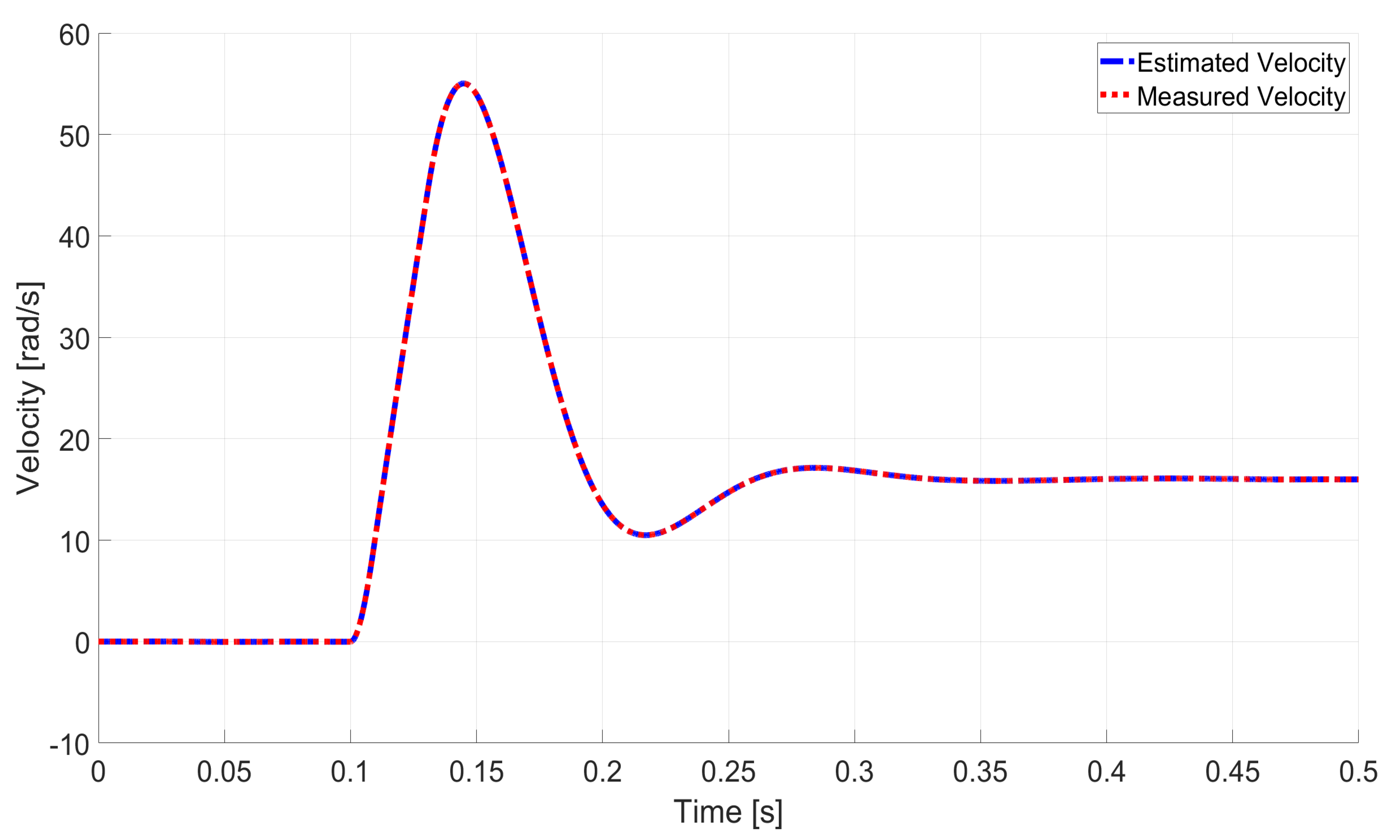
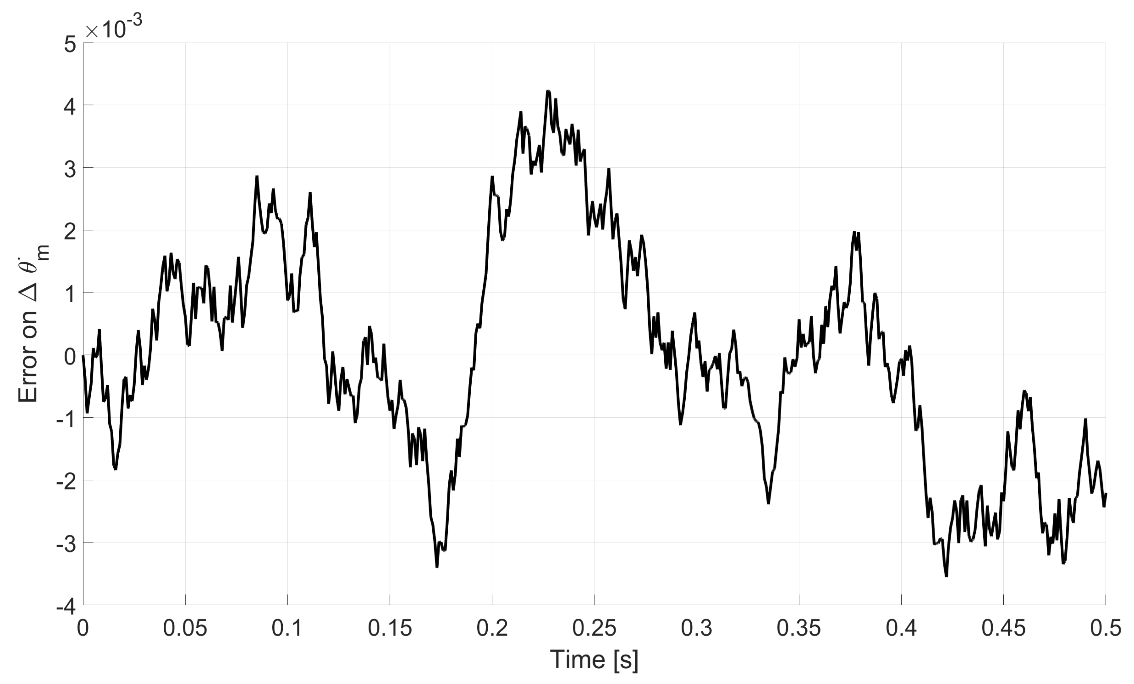
Figure 18.
Brush-less DC Motor velocity: measured and estimated.

Figure 19.
Error between the measured and the estimated values of .

Figure 20.
Torque exerted by the brushless DC motor.


Table 1.
Definitions of parameters and variables used in the dynamic model.
| Symbol | Quantity | Unit |
|---|---|---|
| Torque generated by brush-less DC motor | ||
| Friction between brushless DC motor and gearbox | ||
| Angular position of brushless DC motor | ||
| Angular velocity of brushless DC motor | ||
| Angular acceleration of brushless DC motor | ||
| Inertia of brushless DC motor | ||
| Inertia of gearbox transmission | ||
| Gearbox stiffness | ||
| Gearbox ratio | ||
| Gearbox damping | ||
| Gearbox friction | ||
| Angular position of torque sensor internal ring | ||
| Angular velocity of torque sensor internal ring | ||
| Angular acceleration of torque sensor internal ring | ||
| Inertia of torque sensor internal ring | ||
| Torque sensor damping | ||
| Torque sensor stiffness | ||
| Angular position of torque sensor external ring | ||
| Angular velocity of torque sensor external ring | ||
| Angular acceleration of torque sensor external ring | ||
| Inertia of torque sensor external ring | ||
| Equivalent damping between trunk and exoskeleton | ||
| Equivalent stiffness between trunk and exoskeleton | ||
| Angular position of human trunk | ||
| Angular velocity of human trunk | ||
| Angular acceleration of human trunk | ||
| Human trunk inertia | ||
| Human hip damping |
Table 2.
Bond graph variable analogies.
| Energy Domain | Effort Variable | Flow Variable |
|---|---|---|
| Electrical | Voltage | Current |
| Mechanical | Force | Velocity |
| Hydraulic | Pressure | Volume flow |
| Thermal | Temperature | Entropy flow |
Table 3.
Main component used in the experimental setup.
| Component | Model |
|---|---|
| Brushless DC Motor | Maxon-EC 90 flat, 90 Watt |
| Gearbox | Harmonic Drive, SHD-25-160-2SH-SP |
| Torque Sensor | ME, TS110a ± 100 Nm |
Publisher’s Note: MDPI stays neutral with regard to jurisdictional claims in published maps and institutional affiliations. |
© 2020 by the authors. Licensee MDPI, Basel, Switzerland. This article is an open access article distributed under the terms and conditions of the Creative Commons Attribution (CC BY) license (http://creativecommons.org/licenses/by/4.0/).
Share and Cite
MDPI and ACS Style
Shojaei Barjuei, E.; Caldwell, D.G.; Ortiz, J. Bond Graph Modeling and Kalman Filter Observer Design for an Industrial Back-Support Exoskeleton. Designs 2020, 4, 53. https://0-doi-org.brum.beds.ac.uk/10.3390/designs4040053
AMA Style
Shojaei Barjuei E, Caldwell DG, Ortiz J. Bond Graph Modeling and Kalman Filter Observer Design for an Industrial Back-Support Exoskeleton. Designs. 2020; 4(4):53. https://0-doi-org.brum.beds.ac.uk/10.3390/designs4040053
Chicago/Turabian StyleShojaei Barjuei, Erfan, Darwin G. Caldwell, and Jesús Ortiz. 2020. "Bond Graph Modeling and Kalman Filter Observer Design for an Industrial Back-Support Exoskeleton" Designs 4, no. 4: 53. https://0-doi-org.brum.beds.ac.uk/10.3390/designs4040053