Resolving Energy Losses Caused by End-Users in Electrical Grid Systems


1
Entrepreneurship, Commercialisation & Innovation Centre, University of Adelaide, Adelaide, SA 5005, Australia
2
Faculty of the Professions, Adelaide Business School, University of Adelaide, Adelaide, SA 5005, Australia
*
Author to whom correspondence should be addressed.
Designs 2021, 5(1), 23; https://0-doi-org.brum.beds.ac.uk/10.3390/designs5010023
Submission received: 10 February 2021
/
Revised: 13 March 2021
/
Accepted: 16 March 2021
/
Published: 22 March 2021
(This article belongs to the Section Electrical Engineering Design)
Abstract
:This study utilises the Pareto approach to highlight the energy losses that mainly originate from the phenomena of tiny, initiated events created by end-users of electricity in Australia. Simulation modelling was applied through two stages to examine residential households’ electricity consumption behaviour in New South Wales, Australia. Stage one analysis applied Hierarchical agglomerative clustering and a dendrogram to denote the respective Euclidean distance between the different clusters. Heat maps and threshold value area charts were used to compare the mean power demand for six respective clusters. Stage two used ‘sensitivity analysis’ to investigate how uncertainty in the electricity demand can be allocated to the uncertainty of energy losses. The findings envision practical solutions to dealing with the variability of energy losses and the proposal to set new demand-side strategies associated with individuals. Retail prices of electricity in Australia have risen by roughly 60% since 2007. The research contributes to knowledge about the roots of energy losses in Australia, creating a $210M cost value. Energy losses are of significant economic value, while also impacting energy security. The first limitation of this study is using approaches from complexity theory to grasp the philosophical issues behind the research design and clarifying which insights suit what kind of evidence, thus identifying the data that needed to be collected. The second limitation is that this study’s methodology used a mostly quantitative approach that describes and explains a complex phenomenon in depth more than exploring and confirming that phenomenon. The third and final limitation is that this study’s context is also limited regarding selected sample criteria. The context is limited to a particular demographic area in New South Wales (NSW) in Australia and is also limited to residential houses (not industrial or commercial), which was opposed by data availability and access. The research draws on ‘peak and off-peak’ scales of electricity demand cause energy losses. The research shows the role of the phenomena of spontaneous emergence as a non-linked constraint which is the main issue that splits the optimal solution into pieces and significantly complicates the solution task. Demand side management (DSM) of electricity can be improved from this to construct new demand-side strategies. The study is structured around understanding the consequences of the scalability of events and the clustering dynamic of non-linearity through relevance complexity concepts exclusive to spontaneous emergence (SE), power laws (PLs), Paretian approach (PA), and tiny initiated events (TIEs). We examined the issues of the spontaneous emergence of non-linear, dynamic behaviour involved in the electricity demand of end-users on the basis of pushing individual systems of end-users to the edge of self-organised criticality (SOC). Revising the demand system’s complexity has value in constituting a core domain of interest in what is new in the field of demand side management (DSM), thus contributing to understanding end-users’ behaviour-driven energy losses from both theoretical and empirical perspectives.
1. Introduction
The increasing global population brings with it an increasing energy demand [1]. It has been predicted that the global demand for electricity generation will increase from 20,302 billion kWh in 2014 to 30,364 billion kWh by 2030 [2], based on a demand increase of 2.4% per year [2]. Global dependence on fossil fuels, with over 70% of global electricity generated using fossil fuels, has been widely criticised due to environmental impacts of exponentially increasing atmospheric carbon load resulting in climate warming [3]. Therefore, a number of strategies to move towards decarbonisation of the global economy have been put forward, including renewable energy sources and nuclear technology [4]. However, regardless of the decarbonisation path, there is a need to address electrical systems’ efficiency to reduce energy losses and maximise grid performance [5].
The basis of the electricity grid system is a complex adaptive system (CAS) comprising electricity generation, economic markets, physical networks, and end-users, i.e., multiple, heterogeneous interacting agents [6,7,8,9]. Revising a system’s complexity can have value constituting a core domain of interest (end-users of electricity) to bring to light extension strategies to impose new structures on the field of study of demand side management (DSM), such as (i) establishing a deep understanding of the nature of the relationship between end-users’ behaviour and a complex system; (ii) comparing the degree and the impact of end-users’ behaviour at micro levels in electrical smart grid systems; and (iii) generating insights on how complexity theory is able to enforce needed changes in a complex system with respect to addressing internal problems and fostering new solutions so that the system can realise higher levels of performance in the future [10].
DSM is responsible for monitoring, controlling, and automating the electricity demand side to incubate the demand behaviour (end-users). It relies on reactions of collective autocatalytic subsets (end-users) that have the nature of subtleties arising only on a micro-scale level such as a household and absent at a macro-scale level such as electrical distribution/retailing, transmission and generation [11]. A disproportionate behaviour of households/end-users/micro-levels is one of the main sources of energy losses. Several empirical and theoretical studies previously targeted the DSM of electricity, always to understand how energy losses in the electrical smart grid system may be reduced, and performance improved [12,13].
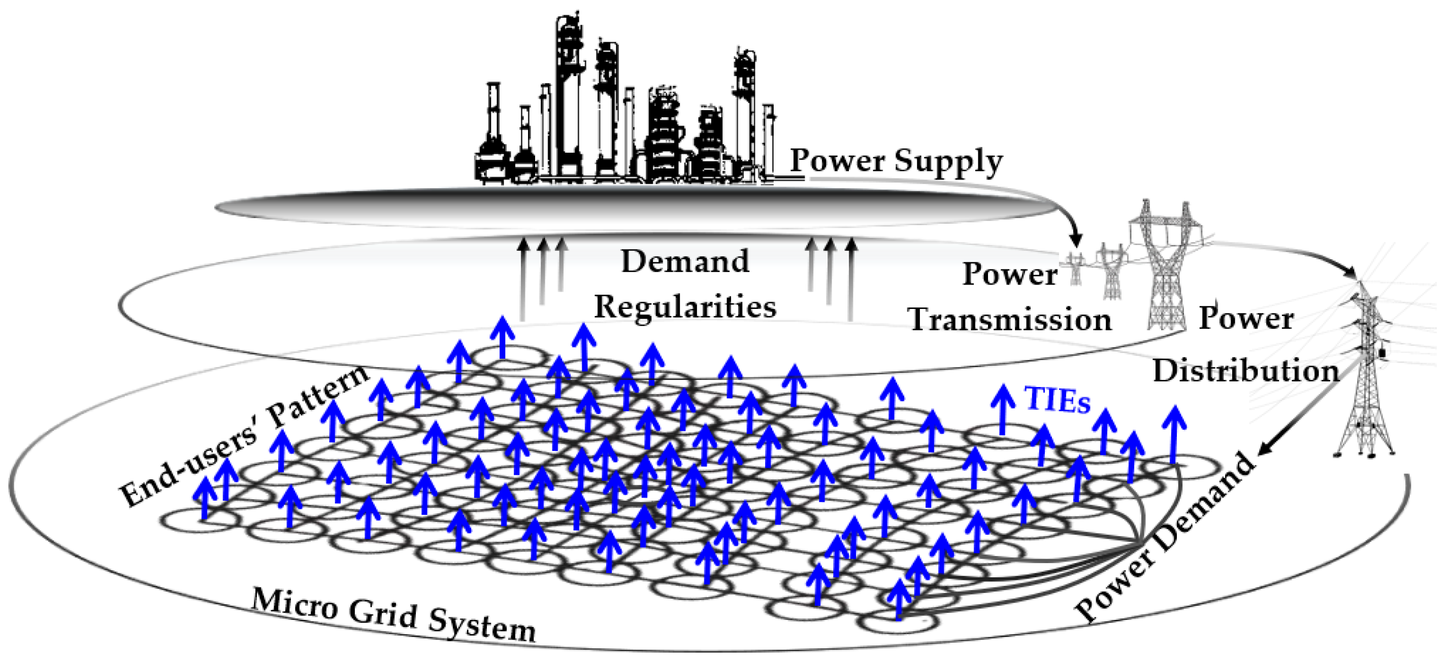
The high complexity of the demand system increases potential energy losses during peak and off-peak consumption, and there is a need to address this issue through socio-technical mechanisms (see Figure 1). There is much redundancy in how unrelated individuals are consuming energy. For an individual household system to sustain itself, a lot of external energy is essential, as there is very little recycling of energy usually available at the household level [14,15,16]. Thus, this study aims to provide contributions based on how to understand end-users’ behaviour in relation to energy losses.
The paper started with an overview of the electrical smart grid system principle in terms of both technical and social concepts. The following two sections introduce the real-life model of the electricity demand of 290 residential houses and exhibit the research methods. Following that, comprehensive definitions introduced the relevant complexity concepts on spontaneous emergence, power law (PLs), and Paretian behaviour of human actions. These key concepts of complexity help to understand the consequences of event scalability and the clustering dynamic of non-linearity. A conceptual model has been hypothesised and empirically tested, using simulation modelling covering 10,512,000 data items distributed closely within the same region [17].
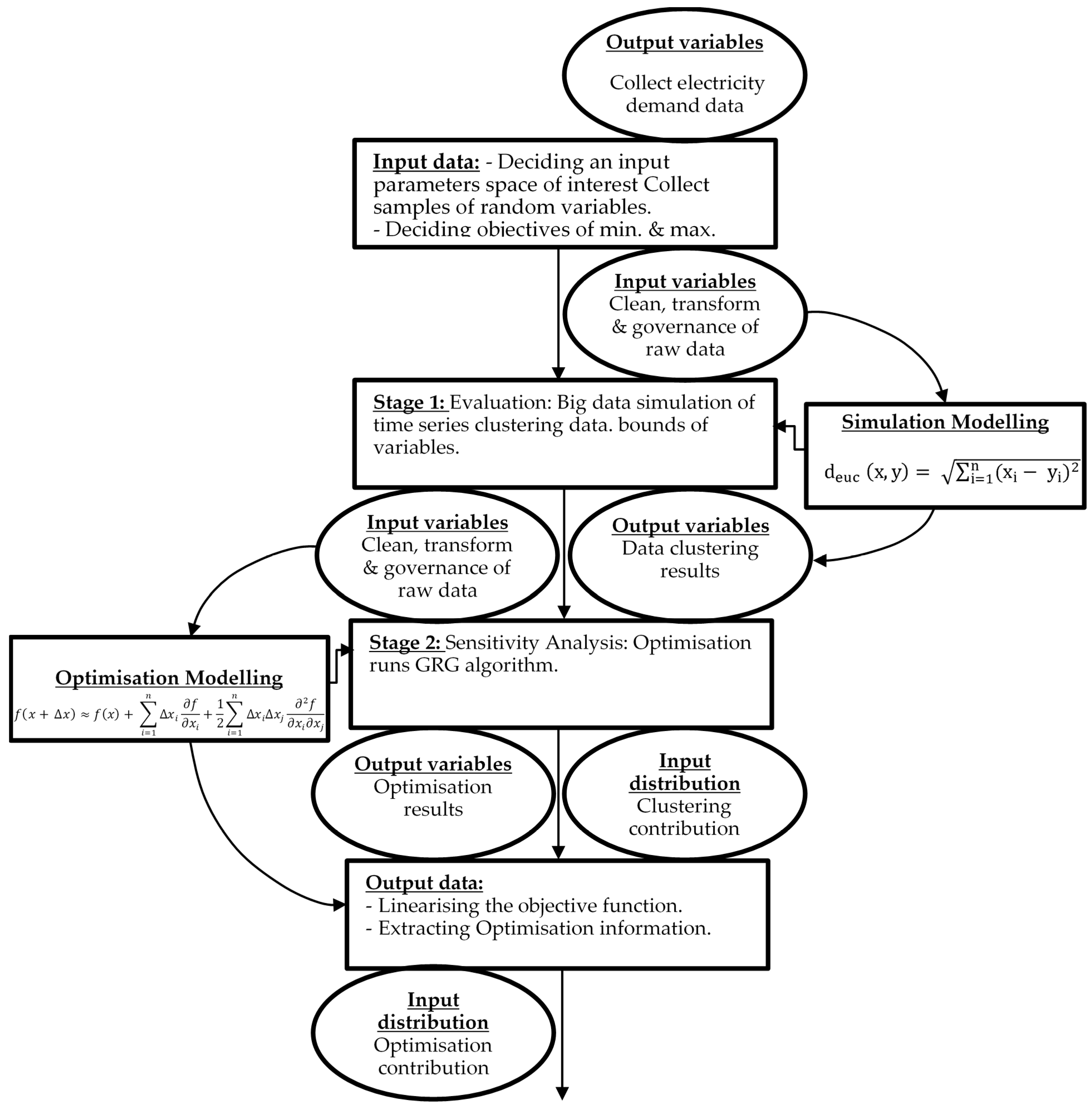
The study investigated the process and the key determinant factors of residential homes in electrical smart grid systems. This study also emphasised residential households’ roles in this process; explored what constitutes electrical smart grid optimisation; and described the operational drivers that lead to desirable grid optimisation (average demand) to mitigate energy losses. Figure 2 below illustrates the existing top-down structure of this study and the relationships of different applied techniques. The input of the large sample size was selected to review the maximum variation and examine the phenomena of emergence in diverse contexts while identifying solutions between different patterns that ‘cut across variety’. The typology of the case study stated is likely to follow various analytical layers.
The first stage in this research was to verify the individual and clustering effects of human behaviours while consuming electricity in Australia’s complex grid system. Python programming language was used for simulation modelling to examine residential households’ electricity consumption behaviour in New South Wales (NSW), Australia. Hierarchical agglomerative clustering (bottom-up approach) was applied to create clusters by partitioning the datasets into different groups according to the degree of dissimilarity among clusters while maximising the similarity within the clusters. A Dendrogram diagram was obtained after hierarchical agglomerative clustering of the time series data to denote the respective Euclidean distance between the different clusters. A heat map was obtained after the Dendrogram diagram wherein each plot displays the mean daily power consumption by each of the residential houses for six respective clusters. Each heat map denotes the percentage of houses contained in each cluster (similar demand). The line plot in heat map diagrams displays the mean power consumption across all houses in a single cluster. In the final statistical test in stage one, we divided the sample into 29 tiers to compare and measure the error occurrence rate attributed to the cyclic peak and off-peak demands. Stage two used ‘Sensitivity Analysis’ to investigate how uncertainty in the electricity demand tends to drive variation in the outputs and leads to electricity losses.
2. Review Actual Demand Data
Sample households were within the same geographic region [17]. Time series data of controlled-load profile (CL) and general consumption load profile (GC) used for analysis were denoted to every half an hour and consisted of a time interval of 48 demand activities. Those are repeated for 290 individual consumers along 365 days with a total amount of data of 10,161,600. The consumption relationships amongst all consumers are built on three parameters: AV, l and u, as shown in Figure 3 (Simulation and Optimisation Module). The previous studies of energy loss caused by end-users’ demand rarely provide complete justification and lead to change in the relative ranking of alternative solutions [18]. This real-life model of the electricity demand of 290 residential houses has been tested to assess the levels of independencies and occurrence of energy losses by each end-user and its half-hourly demand influence on the grid performance.
3. Methods
The analysis in this study is organised into three stages. Pre stage one focuses on sampling size, data cleaning and model designing summarised in Figure 2 and Figure 3. The first stage presents the initial simulation results to differentiate between the mass clustering of various groups with similar electricity demands, in contrast to the targeted goal of identifying whether the electricity grid systems are at risk (energy losses) because of end-users’ demand (see Figures 5 and 6). In stage two, we use ‘sensitivity analysis’ to investigate how uncertainty in the electricity demand (input variables) tends to drive variation in the outputs and leads to electricity losses, affecting the model outputs’ optimisation [19]. Using different tiers or groupings of end-users is needed in this study to add additional heterogeneity where it can be useful in capturing key differences between sub-populations of electricity demand and grid response (see Figure 2 and Figure 3). The model has been parameterised at micro levels to represent electricity losses based on end-users’ behaviours. This preliminary result presents the range of the financial effects and estimates the economic costs of inputs based on the consequence of outputs of the electricity demand model. Finally, this study concludes and draws possibilities for further future study and investigation.
Stage 1 simulation modelling of time series analysis involves studying a sequence of observations collected and ordered in time. Time-series clustering is the grouping of objects with maximum similarity within a group and minimum similarity with other groups or clusters [17]. Unsupervised time series learning, i.e., where time-series do not have labels associated with them, unravels the underlying undiscovered patterns hidden in time-ordered data. Clustering time-series data has been studied extensively in various fields, such as sales data, stock prices, currency exchange rates, weather data, biometrics, and particle detection in physics.
Time series analysis is highly complex due to the large data dimension associated with it [20]. In order to reduce complexity, a time series is usually applied to some representation scheme such as discrete Fourier transform (DFT), discrete wavelet transform (DWT), piecewise aggregate approximation (PAA), trend extraction (TE), complexity-invariant distance measure (CID), temporal correlations (TC) etc. (for details, see references: [21,22,23,24,25]). In this analysis, we compute the distance between two sets of vectors and applied trend extraction in conjunction with Euclidean distance as a similarity measure to cluster the time series database defined by
where the sum is over all the observations and x, y denotes the two-time series (or two sets of vectors) of equal length n over which the distance is calculated by comparing time point (i) of time series x with the same time point (i) of time series (y).
We applied agglomerative hierarchical clustering (which is a bottom-up approach where each low-level cluster is merged together until all the points end up in a single cluster) using Ward’s maximum variance objective, which relies on minimising the intra-cluster variance and maximising the inter-cluster variance. This clustering was effectively visualised using dendrogram, heat maps, and threshold value area charts (see Figures 10–12) and defined by
where is the distance between two clusters A and B denote the increase in squares’ sum resulting from merging two clusters. is the centre of the cluster and n presents the number of points in it. In addition, we presented the heat map of the electricity demands for each of the clusters across one year. Comparing the clustering of samples in terms of energy consumption revealed the degrees of intensity of end-user behaviours’ non-linear dynamics.
Stage 2 of Sensitivity Analysis in linear optimisation applying sensitivity analysis in this study provided insight on how uncertainty in the input variables impact the model outputs to clarify which input variables are driving variation in the outputs [26]. We used a generalised reduced gradient algorithm (GRG) to reveal the non-linear optimisation problem of end-users’ demand [27,28,29,30].
Here:
X: n vector of non-basic variables (desirable average)
Y: m vector of basic variables (original data)
li: Off-peak demand
ui: Peak demand
g: Gradient vector
H: Hessian matrix
m: Basic variables (original data)
n: Non-basic variables (optimisation results)
f: Objective function
EU: End-Users
OCGT: Open cycle gas turbine
CCGT: Combined cycle gas turbine
CP: Coal plant
DCBO: Dispatch cost before optimisation
DCAO: Dispatch cost after optimisation
OG: Optimisation gain per 290 EU
GG1: Storage batteries at home
GG2: Solar panels at home
Minimise f(x)
Subject to gi(x) =0, i=1, m
g (y, x) = 0
g = (g1, …, gm)
f(x) = f(y(x), x)
Normalise F(x)
Subject to li ≤ Xi ≤ ui, i = 1, n
Assuming m ≥ n implies a unique solution (infeasible problem perception)
Testing the optimality of the new results of Xi = (yi, xi)
OG = DCBO − DCAO
Further research is needed if a non-optimal solution resulted from the analysis when the ranges of none basic values violate the desired bounds for unmet system constraints. Then a new optimisation attempt must be made by restarting from step (1), to which new iterative functions of F(x) and y(x) will be applied. However, it is a conditional procedure to keep the original optimal set of (i = 1) as it is, subject to li ≤ Xi ≤ ui.
Where li and ui are the vectors of maximum and minimum bounds for i, thus, we are using GRG algorithm of sensitivity analysis for the problem denoted in the form Equations (1)–(3) by optimising the sequence of problems of the form in Equations (7)–(8). We already have the values of the basic variables y(x) (end-users’ demand).
4. Power Laws (PLs)
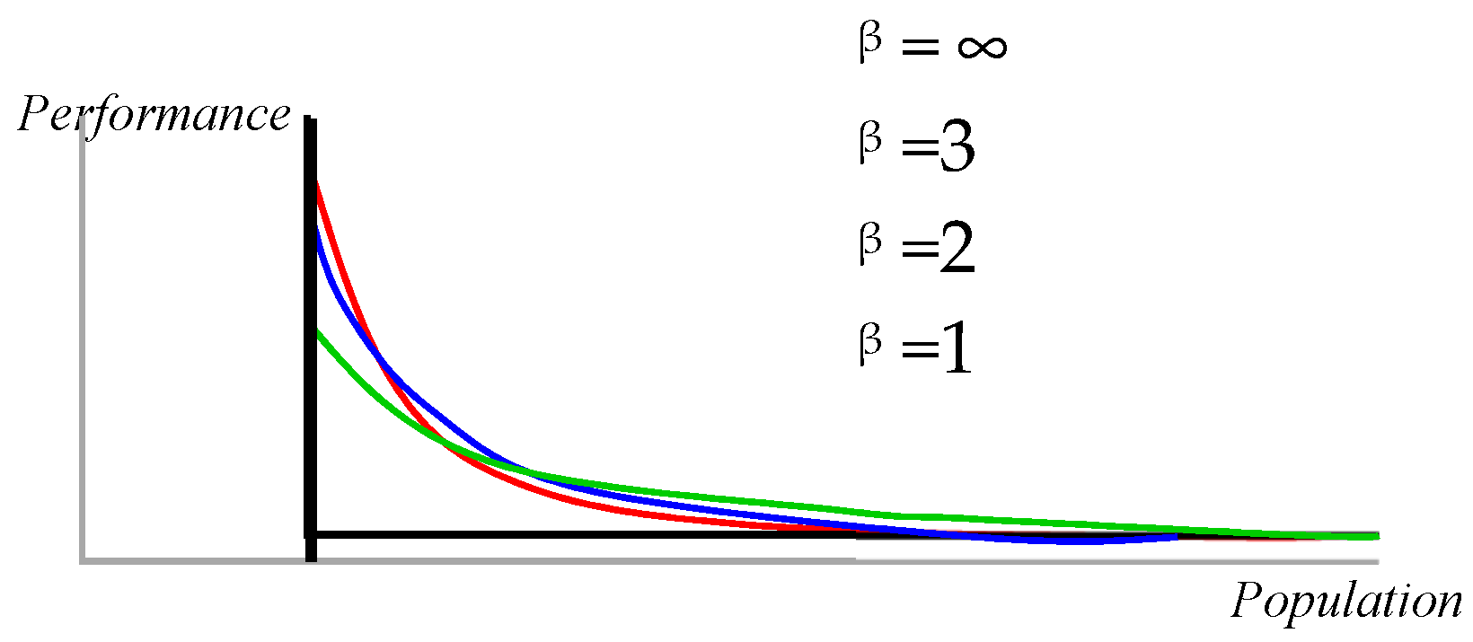
Technology developments create a more complex world which behaves according to scale-free dynamics and indicates the existence of PLs [31]. PLs are built to bind two quantities and define their functional relationship when a relative change first happens to one of them (Figure 4 and Table 1). Accordingly, the relative proportional change in one of those related quantities leads to change in the other. Following this, one of the two initial sizes of quantities will take the initiative to make its independent change, and then the change maker of quantity will power the other one [32,33,34,35,36,37]. Therefore, end-users (societal) in electrical smart grid systems (technical) are a dynamic social case to show the intuition of low occurrence frequencies from a Paretian point of view.
Pareto’s topological metrics are considered to quantify time series data of electricity consumption of residential houses area networks. In the perfect scenario, planning would be so simple and easy as every bug would be treated from the standpoint of being equally important, and every agent would be expected to contribute the same amount of units. As the central point for each unit of inputs, the crux does not contribute identically the same amount of “outputs”, and it leads to the fact that most of the relations in a system are not 1/1.
Knowing this fact, the Pareto principle’s observation reveals most things in life are not distributed evenly. The Pareto principle is a helpmate to stabilise the relationship between the majority of outputs and the minority of inputs. As such, each unit of performance at a particular time will be separately counted as it does not contribute the same amount. Therefore, Pareto’s perception anticipates as a window to realise the kinks in the micro-scale levels based on whom to reward and whom to fix [39].
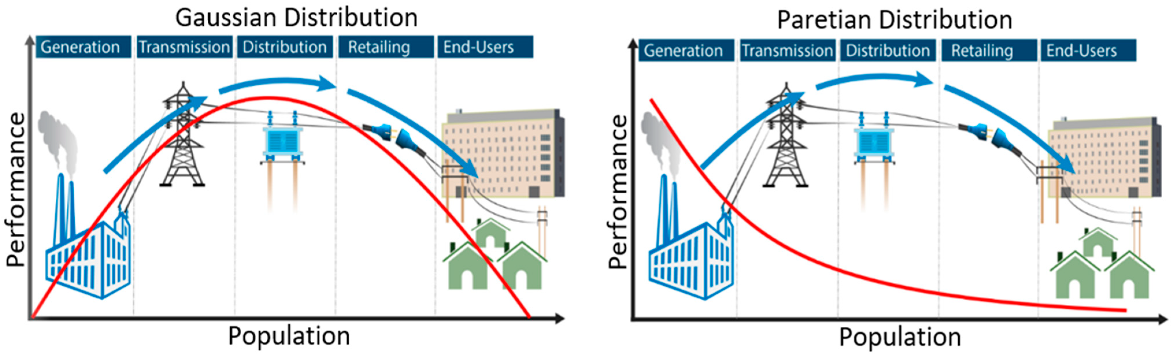
Pareto, or multi-objective, optimisation is a modelling approach useful for multiple criteria decision making, involving more than one objective function to be optimised. We selected the Pareto optimisation approach as a platform for this study because we sought a trade-off between conflicting objectives [40], i.e., minimising energy losses, while maximising grid performance. The Pareto power-law approach facilitates the study of complex systems by focusing on the two tails of extreme measurements or observations, rather than mid-range, average measurements, focusing on the Gaussian approach (see Figure 5). In Power Laws, they are two extremes capturing the distributions that make the whole system act between them [41]. The two extremes in a system seem to be the whole entity that forms the ends. Extremes are the natural attractors’ sources in a limited variance phenomenon [42].
Contrary to the Gaussian approach, the Paretian approach’s standpoint offers different strategic plans that focus on tails, where minimum levels exist between variables [20,21]. Decentralising the nature of end-user demand in an electrical smart grid system is complex and related to the Paretian approach. We focus on visualising the perceived internal and external locus of causality in electrical grid systems and define whether controllable or uncontrollable end-users provide the solutions to electricity issues and failure. Apart from this, we plotted the main technical and social factors that influence electricity losses in the grid system and found that as population (number of people and grid system components) increases, grid performance decreases due to electricity losses.
Paretian distribution in Figure 3 illustrates optimum performance where electricity generation is located (X-axis) due to negligible losses based on small human and technical populations. The point of low performance at the other ‘tail’ is the point of highest populations and end-users’ location (Y-axis). Our proposal widens the distance between the nature of any reality and a Gaussian approach as it always accounts for average results. Gaussian and Paretian strategists do not have the same view of the probability of human events. The interdependencies initiative exhibits signs that are more related to Paretian dynamics and PLs [43]. These elements that make up the ubiquity of PLs activities still exist around the supply/demand of electricity in smart grid systems. Therefore, “Pareto-driven-ideas” are still valid to build new models and frameworks to make sense of the emergence of power laws or what is known as a scale-free theory. The study of (PLs) science sheds light on the scalability process and extreme events induced by (TIEs).
5. Results and Discussion
The electricity demand data shown in Figure 6 and Figure 7 obtained in this study were data collected from the Australian Energy Market Operator (AEMO), as actual demand data.
Data have been collected from residential houses that received electricity from electricity retailers under the AEMO in New South Wales [45].
The sample size in Table 2 and Figure 9 has been generated with a 99% confidence level and 1% confidence interval [44,46]. This means that the 218 residential houses’ results will be considered the lower limit in the research analysis.
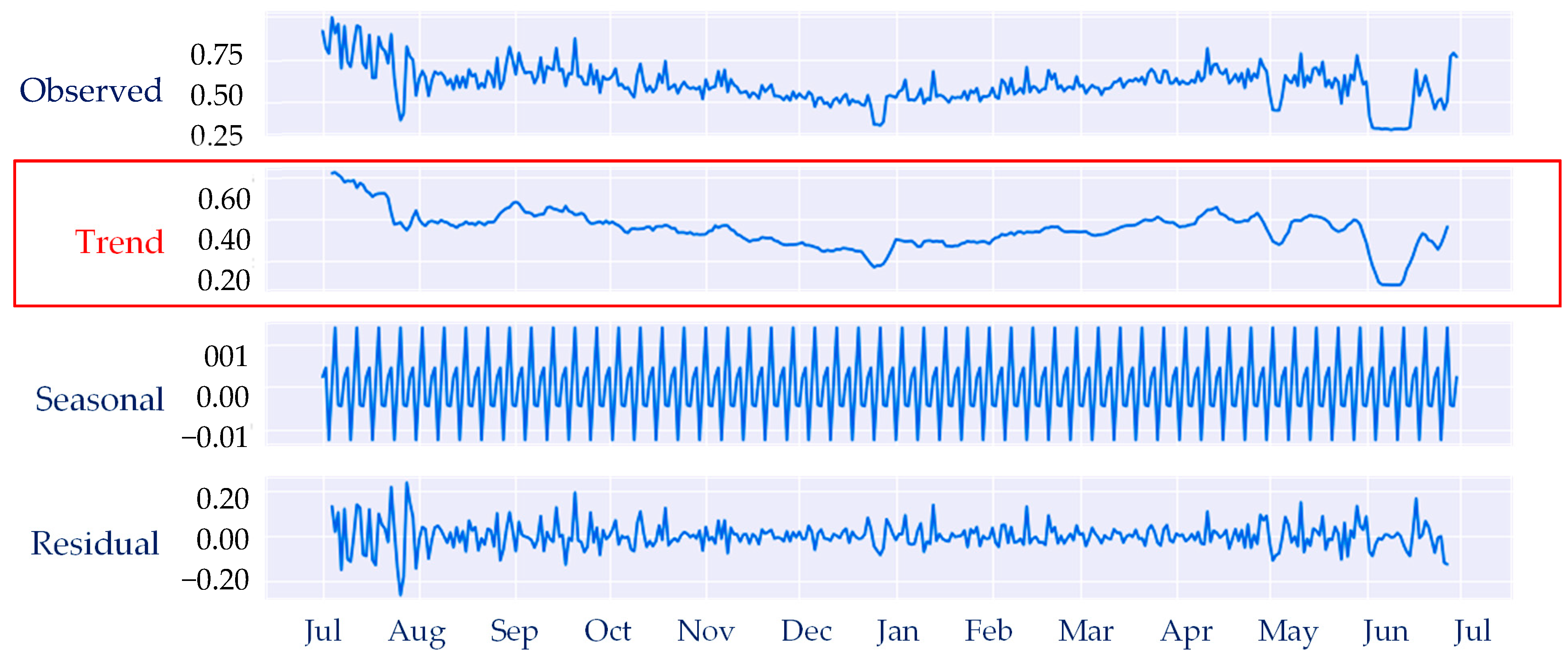
Since we focus primarily on the residential houses’ consumption behaviour, we consider the ‘trend extractions’ as the representations of all the time series in our database (see Figure 8). For the purpose of this study analysis, the timely half-hourly demand for electricity has been selected, and indicative loss costs have been estimated. This study’s scope provides the effectual factors causing loss costs at a very tiny scale (half-hourly demand), covering all other higher scales of the weather, seasons, public holidays, etc., unintentionally. Thus, there is no intention to cover residuals and seasonality in this study through the correlations between different cyclical activities with the weather, seasons, public holidays etc., which could be the subject of future further detailed and complementary study.
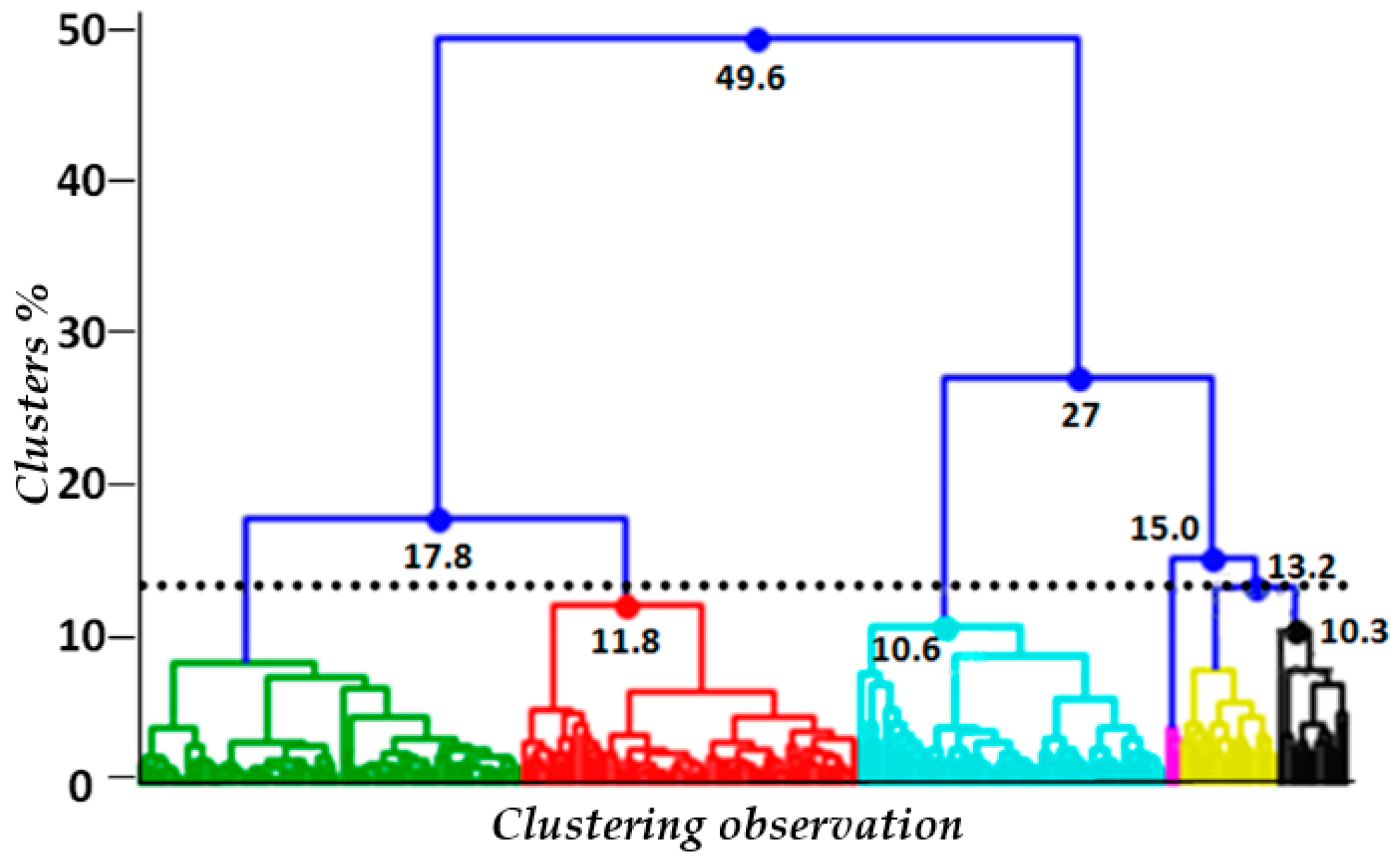
This study examined end-user behaviour in the grid system using data from 300 households in the NSW grid system [45]. Our analysis grouped electricity usage patterns of individual households in clusters of households with similar characteristics. Examination of electricity demand was conducted for each cluster using a Euclidean distance-based similarity measure with trend extraction for representing the time series [47,48]. The hierarchical agglomerative clustering shows six clusters for each time series (year) examined (Figure 9).
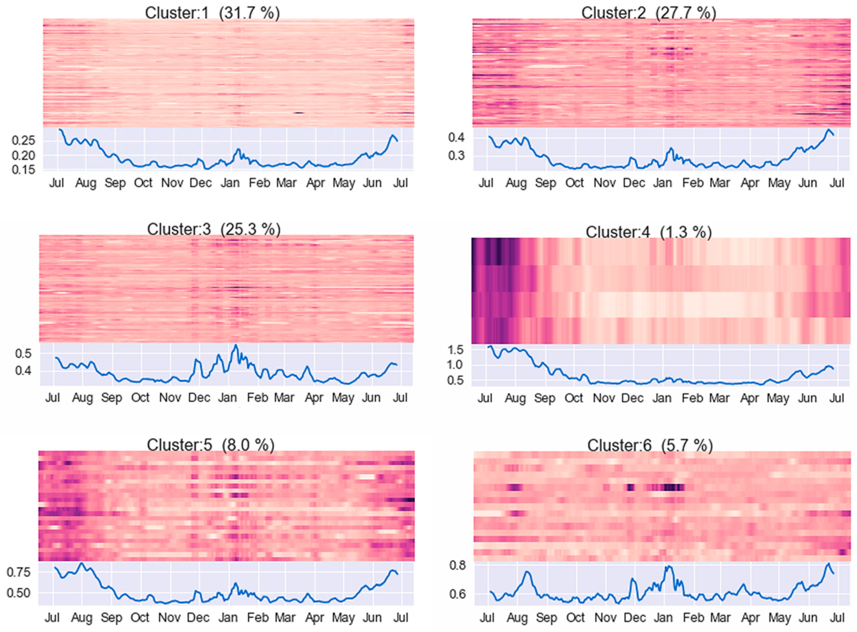
Heat maps are produced to show (mean) daily electricity consumption of each residential household for respective clusters. A darker colour denotes high consumption, while a lighter colour denotes low consumption. The line plot below the heat map shows electricity mean consumption for all households in a particular cluster. This is particularly helpful in validating cluster quality. In each plot, the plot’s darkness or lightness is across the vertical column, which indicates that consumers in a particular cluster follow the same electricity usage pattern.
As shown in Figure 10, we found that household electricity usage clusters have similarity within a cluster, but clusters differ from tier to tier. For example, houses in cluster 1 display low electricity consumption with a maximum mean of around 0.30 units from June to August, with other months showing lower consumption. On the other hand, cluster 6 displays households with high electricity consumption with a minimum of around 0.6 units and a maximum of 0.8 units. A comparison of clustering results reveals that high heterogeneity is a constant between clustered groups (see Figure 11).
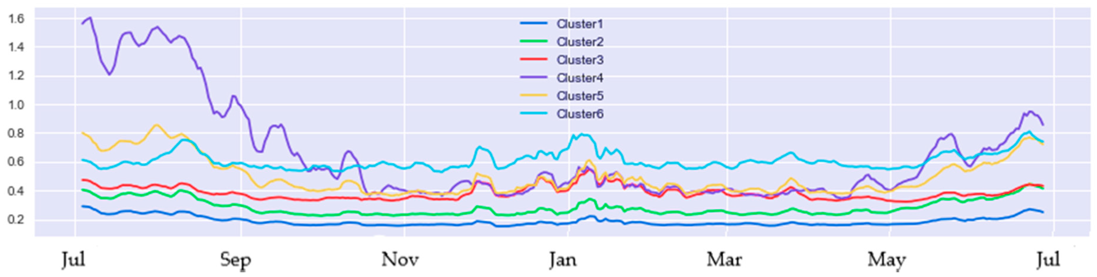
We displayed the power demand behaviour variations within a particular cluster over a single year. The result shows a wide range of electricity consumption by houses which varies from the lowest recorded rate to the highest recorded rate. In relation to the limits of peak and off-peak scales of power rates, we find that the power demand has quite as much variance even within a single cluster. One argument is that individual consumers are predisposed to autonomous regimes’ perspective by having the freedom to control their own affairs and govern themselves according to their desires. This study’s debate mainly revolves around whether the perception of modelling end-users’ demand drives the relationship to make the grid system liable to solve energy losses. Based on the demand data, it has been investigated whether the variance of each two demands (li,& ui) share equal importance or maybe are entirely uneven.
Further evaluation by utilising modelling simulation was performed using the module as illustrated earlier in stage 1 Figure 3 to support the findings of similarity measures () for each demand activity li ≤ Xi ≤ ui, i = 1, n. The model performs the following calculation steps, as shown in Table 3 and Figure 13: (1) Compute demand (t) for interval time i, and calculate values of li, ui, AVi for each end-user; (2) Statistically define the influence states of events/losses (li & ui) and no events/no losses (AVi) which satisfies data confidence level (α ≈99%). Our baseline variable values were orderly selected for (li, AV & ui). The simulation model was able to generate ranges of “false events” (li & ui) and “true events” (AV) demand, and probabilistic information was extracted where each customer and each half-hourly demand represents a unique influence towards objective functions f(x). A first look between the distribution of results and the central limit theorem of (li, AV & ui) would identify the output variables (Y: m vector of basic variables of original data), since the occurrence of (AVi) true events (denoted by black dotted curve) was found from 5039 to 24,130 units, e.g., AVi ≈ 4.76–22.81%, whereas this was dominated by both occurrence ranges of (li) false events (blue dotted curve) from 43,561 to 89,220 units ≈10.54–38.59%, where also the occurrence of (ui) false events (denoted by red dotted curve) was found from 11,151 to 40,813 units ≈ 41.19–84.35%.
A part of stage one analysis was searching for the influence of clustering behaviour of end-users, and these visual and statistical results state how various independent variables significantly cause energy losses, or to put it the other way around, how sensitive energy losses () to the various demand variables originated from end-users. The weight assigned to each individual in the entire sample distinguishes the interval time of those who do not incur a direct cost of energy losses () and within the desirable demand regime when zero chance of giving rise to energy losses occurs. The black dotted curve in Figure 12 and the computational results in Table 3 illustrate a weakness rate found in end-users’ desirable demand (AV).
Taking into consideration the relations presented between end-users in the previous clustering simulation, one can observe that all output variables in Table 3 have a positively skewed distribution (mean > median) as it can be observed that more than 50% of end-users have higher values of (li) than (AV) and (ui). The conclusion of the stage 1 result leads to a kind of premise that the input of actual demand variables will have a potentially more significant impact on the output variables. This analysis is meant to show the influence of energy losses, with facts to propose expansions in some other directions discussed in the stage 2 analysis.
The second stage in this study uses sensitivity analysis for optimisation modelling to define the probabilistic benefit of optimising individual homes’ demand systems. Based on the same data retrieved from the previous simulation analysis concerning the influence of individual end-user’s factors shaping demand, the analysis investigated three factors: (1) the cost of demand occurrence when (Xi ≤ li, Xi ≥ li, Xi ≤ ui, Xi ≥ ui & Xi = AVi), (2) the cost-benefit analysis of shifting individual demands from (ui) and (li) to (AVi), (3) the optimisation feasibility by reusing the stock available (I = CL + GL) of the same half-hourly demand capacity consumed by individual end-users from the grid. The data sample is divided into 29 tiers by following the analysis steps in stage 2, as illustrated in the flowchart (Figure 3).
The simulation in stage one reveals the actual demand behaviour and demonstrates the effect of . Comparing the two statistical results of simulation modelling and sensitivity analysis in Table 4 and Table 5 can be interpreted in the following way: the optimisation modelling to (AV-true) variables is an adjustment process to the values of AV-true simulation variables upward and downward to achieve an optimum (demand) selection within the same demand capacity of historical data. For the given case study, an optimisation selection bias occurs to the objective function F(x) which tends to act within denoted units of average demand rates (li ≤ Xi ≤ ui, i=1, n) and given that each new demand unit has a (n) vector of none, there are basic variables of desirable average (x). F(x)’s optimisation goal aims to shift the demand system into the desirable bounds (li ≤ Xi ≤ ui).
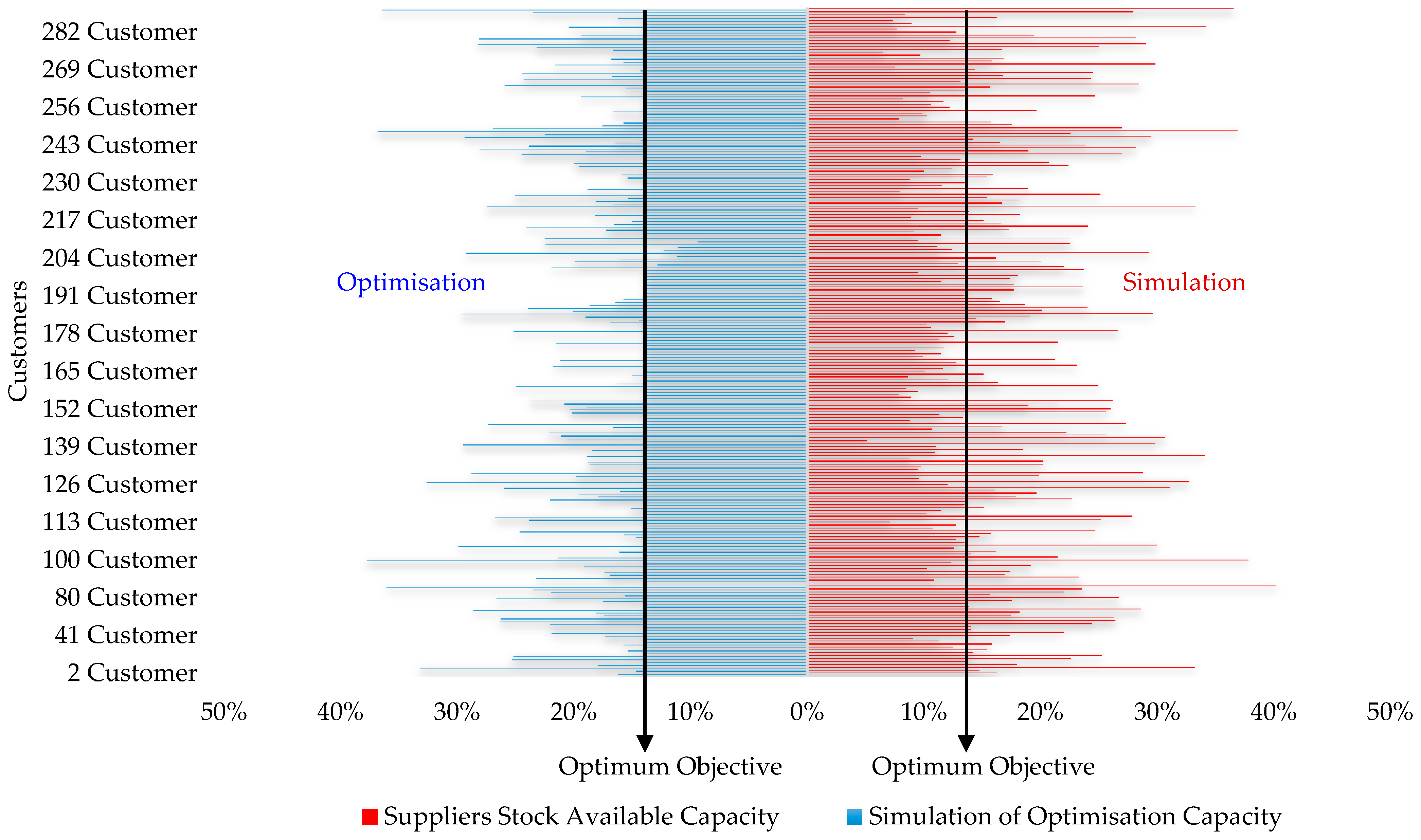
The output of Table 5 can also be shown in Figure 13; the demand optimisation has a significant positive reduction of the influence of (i) and (u) of false demands that reform as 32.76% of the total population demand. That is, the (AV) rate of end-users increased from 10.70% (more gaps—simulation side) to 43.46% (fewer gaps—optimisation side). Given the positive influence of the average estimated demand that does not pose a risk (energy losses), the bounds under this assumption are somewhat more interesting in this study.
In an ideal electricity market, the power plant generation’s expected marginal cost against the electricity price (kg of fuel/KWh of electricity) determines how much profit each power plant should produce. Hence, there will generally be an influence of power generator types compared to the operation cost in a typical electricity market scenario. How large this generation power gap is depends on which and when different power plants participate in primary control demand. This procedure is entirely relying on the technical properties of different power plants (see Table 6). Based on this kind of understanding, we choose to estimate the cost of demand in relation to the combined cost of the generation power system at different loads (AV, l, u). Although we are looking for a more realistic alternative cost figure in the future, it can be achieved directly from the used generation capacity operators in a tight practical situation. Notice that the objective function (li ≤ Xi ≤ ui, I = 1, n) relies on three different kinds of power generation-based cost functions. Therefore, we have modelled the consequences of the cost-based power generation by following the light of the long run marginal cost (LRMC) assigned by Independent Pricing and Regulatory Tribunal (IPART) [14,49], and as concluded in Table 6:
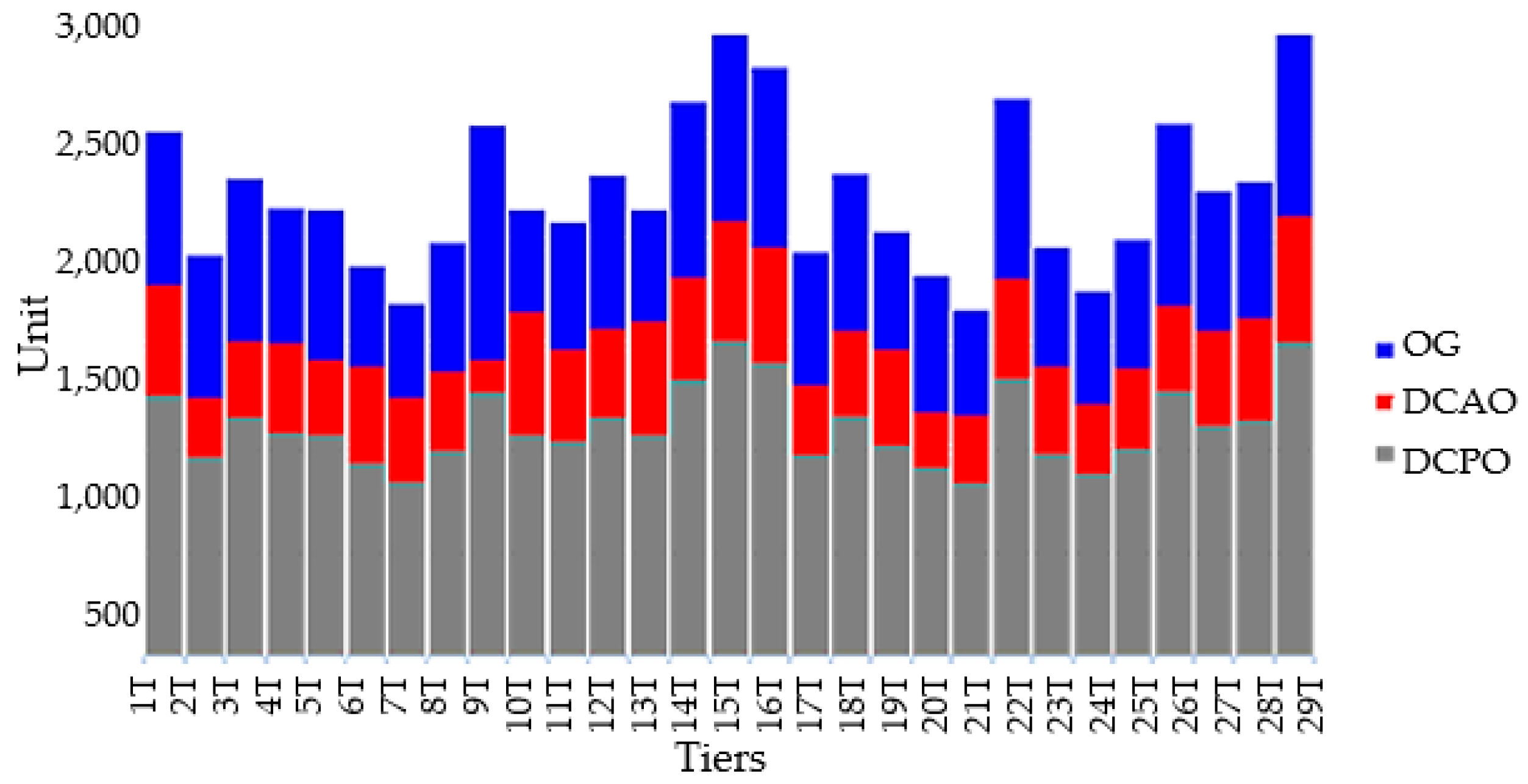
The cost impact of individual end-users’ demand varies from one demand scenario to another demand scenario (AV, l, u) during electricity demand interval times. Accordingly, the sensitivity analysis of optimisation objective function F(x) is used to determine an approximate cost reduction by computing the same electricity demand capacity from the case study data to individual end-users. Thus, F(x) of the scenario problem () includes both the half-hourly demand (CL) and (GL) of individuals either being (AV), (l) or (u). The influence of end-users’ demand resulting in energy losses-based cost is examined by using three parameters of dispatch cost before optimisation (DCBO), dispatch cost after optimisation (DCAO), and optimisation gain (OG = DCBO − DCAO) (Table 7 and Table 8 and Figure 14).
Returning to the optimisation output listed in Table 5, the objective function is set to the (AV) demand, where f(x) = f(y(x), x) and (H = ∂2 f = ∂xi/∂xj) of Taylor expansion of (GRG) are used to change the mean of the distribution by reducing the occurrence of (). To simplify this study’s presentation and make the output results comparable in a more common evaluation environment, we propose using a score matching to compare the output demand data of the optimisation analysis with the real cost trading influenced by CCGT, OCGT and CP (see Table 6). The estimated cost incurred from energy losses varies and depends on the demand’s nature during a time interval, e.g., AV, l, u. This redispatch problem can be too complex if all physical limitations of the generation power system are considered. Thus, at least in this stage of the study, we neglect this complexity, and we assume the scenario cost parameters depend on the variables’ values of the real-time demand which is limited to the price-sensitive load and based on the cost of load capacity factor [14,49].
As far as we can judge, the sensitivity analysis will, however, impact the rate of demand behaviour of individual end-users; hence, as there is a need to estimate the new cost associated with any float of critical activities of energy loss in half-hourly demand, the optimisation modelling is applied. Picking the percentile level of each cost value generated in stage 2, shown in Figure 14 and Table 7, corresponds to 290 end-users. Fitting the cost results of energy loss from a non-linear (DCBO) model with their associated percentile levels to a linear (DCAO) model can be displayed in (OG) outcomes. This gap might jeopardise a profit margin from various individual demands. Table 8 shows the impact of (DCAO) on the original demand (DCBO) by reducing 62.14% of () concurrent with annual profit cost of (¢12,315.92 per 290 of ). Thus, the (OG) identifies “Where is this energy loss coming from?”, or, put the other way around, how much each end-user is mostly responsible for the incurred energy loss (uncertainty). The existing result reveals that energy loss around (¢69.71), caused by capita (end-user) equivalent to the annual ($6.3 m) cost of loss caused by all residential houses in Australia, would probably be more or less.
This proposed method assesses and quantifies the impact of energy losses at individual end-users’ level disregarding any change demand orders. This approach helps solve energy losses and mitigates the conflicts and profit disputes between all electricity stakeholders (suppliers, retailers and end-users). This is because subjective evaluation will be replaced with objective quantification and identification of optimisation values generated by sensitivity analysis. Although the objective function in the optimisation modelling in this study did not include a parametric study of the (GC), (CL) and (GG), we noted that from the optimisation results of the case study, various demands were particularly sensitive to the bidirectional supply of electricity from the grid (GC + CL) and the houses (GG = GG1 + GG2). For that case, the last part of the analysis in this study draws attention to the role of the parametric constraints (GG) at homes regarding the optimisation goal F(x) and based on two factors: (1) The influence of (GG) in individual houses to support systems’ optimisation (Table 9), and (2) The capability of (GG) in individual houses to regulate timely demand for the sake of systems’ optimisation (Table 9 and Table 10).
Binary variable: = 1 when i goes li ≤ GC + CL ± GG ≤ ui, (optimum demand)
Binary variable: = 2 when i goes above ui ≤ GC + CL ± GG ≤ li (none optimum demand)
Based on Table 10, the output shows that we get a significant effect of (GG1) on the rate value of 0.8965. That is, the expected half-hourly participation is 89.65% to keep matching the optimisation demand (li ≤ GC + CL ± GG ≤ ui) during daily demand of interval times. From the same table, (GG2) results were found within a more conservative value of 0.2413 than the value obtained with the (GG1). This is an expected result and the reason that the tendency of (GG2) has no impact during nighttime. In addition, achieving the optimisation objective goal makes the grid supply (GC + CL) have the capability of limiting the participation of (GG2). The expected half-hourly participation of (GG2) is 24.13% that is also to keep the system matching the goal of the optimisation (li ≤ GC + CL ± GG ≤ ui) during daily demand of interval times.
6. Need for Future Research
Whilst energy loss is a multiarea problem, we assume the optimisation solution we have provided is a single player that can only propose an objective function scenario and reuse the same capacity demand to each consumer, but it is not yet able to regulate either downwards or upwards of end-users’ demand. Thus, the conclusion is that the ongoing future studies of energy demand optimisation would aim to divide the time series data into two regulating groups, where the first data group (GC + CL) is the power supply from the grid and its goal is to keep its balance within the ranges of desirable average demand. The second data group (GG) is the power supply from the houses (GG1 + GG2). The central role of this group is to up-regulate and down-regulate timely demand to satisfy the optimal demand goal. Notably, the central dispatch approach via sensitivity analysis that we have proposed in this study tries to maximise the benefit equally to all stakeholders, and minimise the cost of power generation by redispatching the same demand capacity consumed by each end-user.
Further work is needed to focus on the expected capacity of (GG1) and (GG2) at individual homes to serve the demand system optimisation goal. The cost of energy losses can be a significant input to the electrical grid design, operation, and network businesses’ planning. In economic terms, the cost of losses caused by energy losses of end-users’ demand is an appropriate indicator that can be applied to improve performance.
In this study, an effective method based on simulation optimisation is performed to determine the influence of end-users’ behaviour regarding energy losses and the expected cost of losses. This model’s light may be considered a platform to be used further to investigate the root causes and the optimum demand system’s cure from energy losses. The proposed method is applied to obtain the most likely demand performance (li ≤ Xi ≤ ui, I = 1, n) to avoid the demand system probability of failure (). It is found that the optimisation from a non-linear (DCBO) model to a linear (DCAO) model can be displayed in (OG) outcomes as an expected margin of profit from various individual demands. In the meantime, it is found that the demand system optimisation when reusing the same demand capacity of electricity for each end-user (we have to provide exactly the same amount of demand to satisfy each consumer) can partially decrease the probability of energy losses. The optimisation result illustrates a lack of capability of the tested model. Each house has a unique demand and needs a unique optimal trade-off mechanism between the grid power supply and the home’s power generation (solar and storage battery) to balance individual houses up to the objective function. To shed extra light on the above issue, a z test was applied (see Table 11).
H0 = the optimisation ‘mean’ [computed] is equal or above p-value when p ≥ 0.001
H1 = the optimisation ‘mean’ [computed] is below p-value when p < 0.001
α ≈99%
Table 11 summarises the demand optimisation results of 290 end-users. The magnitude of the interest is p < 0.001. The mean (z) is tested from AVmin to AVmax. The average ranges are defined as the optimisation’s objective functions and denoted in the table from (x1) to (x18), where 55.55% of the total sample reject the null hypothesis H0. The significant results of the p-value (P(T<=t) two-tail < 0.001) conclude that there is still a significant difference in a sample mean from the desirable demand average (li ≤ Xi ≤ ui, i = 1, n) where, in turn, the result of the sample mean (µr) does not always support the output of the hypothesised optimisation mean (µo).
7. Conclusions
The output of this result is important as it is a true reflection for multiple numerical models of individual end-users that only a portion of the entire parameter space yields relevant results. It is interesting to define what the behaviour of this proportion is and how, when, and where it is located in the entire parameter space. To reveal the randomness distribution and act of the parameter space of interest (those causing energy losses), we compared the scatter plot, tornado result and dependency result of each tier space (parameter) within the sensitivity matrix requirements. The results showed that the new optimisation distribution of output variables changed for good. However, the optimisation modelling that is unable yet to provide the stability needed in the power domain because a part of this process relies on the availability, capacity, and automative power of renewable energy parameters (solar and storage battery) at individual homes, are all relevant.
The sensitivity analysis approach (SA) has been applied for identifying essential parameters that dominate model behaviours. The utilisation of sensitivity analysis is generally desirable to understand the relationship between input parameter values, output sensitivities, and how these relationships influence model predictions to detect model deficiencies. Because of the relative significance of demand energy losses and attendant costs, the light of sensitivity analysis has been used in this study to find the impact of combined variations of the three main parameters of (GC), (CL), and (GG), that cause a change in the ranking of the three assumed management options of (l), (AV), and (u) during an interval time (n) of electricity consumption. We are altering the ‘Average’ as a preferred management decision since the peak and off-peak demands are permanently defined as unfavourable events. The module in Figure 3 aims to search for and identify optimal plan options of end-users’ demand to maximise demand-side quality and minimise the cost of energy losses caused by (i) and (u) demands of end-users. The optimisation module was developed in two main steps that are designed to integrate optimisation objective function, which is designed to stop/reduce the influence of (i) and (u) demands and reduce the cost of energy losses simultaneously. The optimisation model enables and calculations at a specified confidence level (α ≈ 99%) to define the uncertainty influence of individual end-users of electricity at an unequal iterative demand rate. It can be noted that the optimisation objective is always conflicting. Approximately 62.14% of the 10,000,000 demand events generate energy losses, which means that demand-side optimisation from these unfavourable events was zero value. In comparison, the remaining 37.86% of the events yielded desirable demand (li ≤ Xi ≤ ui, i = 1, n), which is assumed to be of interest in optimising the systems’ output. As a result, only an average of 3,786,000 demand events (out of 10,000,000 total events) can support the systems’ optimisation within the same dispatch stock of half-hourly demand. Models such as the electricity demand model, where the benefit is that the optimisation output values may not achieve optimal results but intend to inform a suite of possible model outcomes that lead to alternatives, can inclusively be parameterised within a new model to mitigate the influence of the energy losses.
Author Contributions
Conceptualisation: A.Z., I.G.; Formal analysis: A.Z.; Investigation: A.Z., Indra Gunawan.; Methodology: A.Z., I.G.; Project administration: A.Z., I.G.; Resources: A.Z. Software: A.Z.; Supervision: I.G.; Validation: A.Z., I.G.; Writing: A.Z.; Writing—review & editing: A.Z., I.G. All authors have read and agreed to the published version of the manuscript.
Funding
This research received no external funding.
Data Availability Statement
Data is contained within the article.
Acknowledgments
We thank Vernon Ireland (The University of Adelaide) and Frank Schultmann (The University of Adelaide) for their supervision and advice, and Pankaj Sharma (The University of Adelaide) for sharing his analytical insights on an earlier version of the manuscript. Additionally, our thanks must go to the Assistance Editor Danae Yu, the Editorial Board and the Reviewers for their guidance and thoughtful comments.
Conflicts of Interest
The authors declare no conflict of interest.
References
- Gigerenzer, G.; Selten, R. Bounded Rationality: The Adaptive Toolbox; MIT Press: Cambridge, MA, USA, 2001. [Google Scholar]
- Colson, C.; Nehrir, M. A review of challenges to real-time power management of microgrids. In Proceedings of the 2009 IEEE Power & Energy Society General Meeting, Calgary, AB, Canada, 26–30 July 2009; pp. 1–8. [Google Scholar] [CrossRef]
- The Australian Academy of Technological Sciences and Engineering (ATSE). The Hidden Costs of Electricity: Externalities of Power Generation in Australia; Parkville: Victoria, Australia, 2009; pp. 1–88. Available online: https://www.applied.org.au/ (accessed on 10 September 2020).
- Fan, Z.; Kulkarni, P.; Gormus, S.; Efthymiou, C.; Kalogridis, G.; Sooriyabandara, M.; Zhu, Z.; Lambotharan, S.; Chin, W.H. Smart grid communications: Overview of research challenges, solutions, and standardisation activities. IEEE Commun. Surv. Tutor. 2013, 15, 21–38. [Google Scholar] [CrossRef] [Green Version]
- Su, W.; Wang, J. Energy management systems in microgrid operations. Electr. J. 2012, 25, 45–60. [Google Scholar] [CrossRef]
- Grid Australia. National Electricity Rules: Distribution Losses in Expenditure Forecasts. 2012. Available online: http://www.aemc.gov.au/getattachment/fc5d7ca3-b07c-405e-84c4-f72bf9b37010/Grid-Australia.aspx (accessed on 15 March 2019).
- Noor, S.; Yang, W.; Guo, M.; van Dam, K.H.; Wang, X. Energy demand side management within micro-grid networks enhanced by blockchain. Appl. Energy 2018, 228, 1385–1398. [Google Scholar] [CrossRef]
- Wu, D.; Radhakrishnan, N.; Huang, S. A hierarchical charging control of plug-in electric vehicles with simple flexibility model. Appl. Energy 2019, 253, 113490. [Google Scholar] [CrossRef]
- Zhang, T.; Pota, H.; Chu, C.-C.; Gadh, R. Real-time renewable energy incentive system for electric vehicles using prioritisation and cryptocurrency. Appl. Energy 2018, 226, 582–594. [Google Scholar] [CrossRef]
- Uhl-Bien, M.; Marion, R. Complexity leadership. In Part 1—Conceptual Foundations; Leadership Horizons Series; Information Age Pub (IAP): Charlotte, NC, USA, 2008; Available online: http://search.ebscohost.com.ezproxy.laureate.net.au/login.aspx?direct=true&db=nlebk&AN=469811&site=ehost-live (accessed on 13 August 2020).
- Steel, M. Self-sustaining autocatalytic networks within open-ended reaction systems. J. Math. Chem. 2015, 53, 1687–1701. [Google Scholar] [CrossRef]
- Liu, J.; Xiao, Y.; Gao, J. Accountability in smart grids. In Proceedings of the 2011 IEEE Consumer Communications and Networking Conference (CCNC), Las Vegas, NV, USA, 9–12 January 2011; pp. 1166–1170. [Google Scholar]
- Yilmaz, S.; Chambers, J.; Patel, M. Comparison of clustering approaches for domestic electricity load profile characterisation—Implications for demand side management. Energy 2019, 180, 665–677. [Google Scholar] [CrossRef]
- Soldatos, P.G. The long-run marginal cost of electricity in rural regions. Energy Econ. 1991, 13, 187–198. [Google Scholar] [CrossRef]
- Wu, J.; Zhang, B.; Jiang, Y.; Bie, P.; Li, H. Chance-constrained stochastic congestion management of power systems considering uncertainty of wind power and demand side response. Int. J. Electr. Power Energy Syst. 2019, 107, 703–714. [Google Scholar] [CrossRef]
- Wolisz, H.; Schütz, T.; Blanke, T.; Hagenkamp, M.; Kohrn, M.; Wesseling, M.; Müller, D. Cost optimal sizing of smart buildings’ energy system components considering changing end-consumer electricity markets. Energy 2017, 137, 715–728. [Google Scholar] [CrossRef]
- Ferreira, L.N.; Zhao, L. A time series clustering technique based on community detection in networks. Procedia Comput. Sci. 2015, 53, 183–190. [Google Scholar] [CrossRef] [Green Version]
- Buza, K.; Nanopoulos, A.; Schmidt-Thieme, L. Time-Series Classification Based on Individualised Error Prediction. In Proceedings of the 2010 13th IEEE International Conference on Computational Science and Engineering, Hong Kong, China, 11–13 December 2010; pp. 48–54. [Google Scholar]
- Lund, H.; Arler, F.; Østergaard, P.A.; Hvelplund, F.K.; Connolly, D.; Mathiesen, B.V.; Karnøe, P. Simulation versus optimisation: Theoretical positions in energy system modelling. Energies 2017, 10, 840. [Google Scholar] [CrossRef]
- Balankin, A.S.; Matamoros, O.M.; Galvez, E.M.; Perez, A. A Crossover from Antipersistent to Persistent Behavior in Time Series Possessing the Generalyzed Dynamic Scaling Law 69. 2004. Available online: https://www.adelaide.edu.au/library/ (accessed on 14 August 2020).
- Wang, X.; Keogh, E.J.; Lonardi, S.; Shelton, C. Data Mining Techniques on Historical Image Databases. 2010. Available online: https://www.adelaide.edu.au/library/ (accessed on 23 July 2020).
- Batista, G.; Keogh, E.; Tataw, A.; Souza, P. CID: An efficient complexity-invariant distance for time series. Data Min. Knowl. Discov. 2014, 28, 634–669. [Google Scholar] [CrossRef]
- Ferreira, L.N.; Zhao, L. Time series clustering via community detection in networks. Inf. Sci. 2016, 326, 227–242. [Google Scholar] [CrossRef] [Green Version]
- McBurney, P.W.; Jiang, S.; Kessentini, M.; Kraft, N.A.; Armaly, A.; Mkaouer, M.W.; McMillan, C. Towards Prioritising Documentation Effort. IEEE Trans. Softw. Eng. 2018, 44, 897–913. [Google Scholar] [CrossRef]
- Spendler, L.I. Data mining and management (Ser. Computer science, technology and applications). Nova Science. 2010. Available online: https://lesa.on.worldcat.org/oclc/753956716 (accessed on 29 July 2020).
- Kuc-Czarnecka, M. Sensitivity analysis as a tool to optimise Human Development Index. Equilibrium 2019, 14, 425–440. [Google Scholar] [CrossRef] [Green Version]
- Ruda, M.M.; Thompson, D.W. Comparison of primal and dual solution methods for the chemical equilibrium problem using GRG and sensitivity analysis. Can. J. Chem. Eng. 1985, 63, 113–121. [Google Scholar] [CrossRef]
- Pirnia, M.; Cañizares, C.A.; Bhattacharya, K. Revisiting the power flow problem based on a mixed complementarity formulation approach. IET Gener. Transm. Distrib. 2013, 7, 1194–1201. [Google Scholar] [CrossRef]
- Proietto, R.R.; Arnone, D.; Bertoncini, M.; Rossi, A.; La Cascia, D.; Miceli, R. Mixed heuristic-non linear optimisation of energy management for hydrogen storage-based multi carrier hubs. In Proceedings of the IEEE International Energy Conference (ENERGYCON), Cavtat, Croatia, 13–16 May 2014; pp. 1019–1026. [Google Scholar] [CrossRef]
- Pal, P.; Bhunia, A.; Goyal, S. On optimal partially integrated production and marketing policy with variable demand under flexibility and reliability considerations via Genetic Algorithm. Appl. Math. Comput. 2007, 188, 525–537. [Google Scholar] [CrossRef]
- Li, M.; Vo, Q.B.; Kowalczyk, R. A Pareto-efficient and fair mediation approach to multilateral negotiation. Multiagent Grid Syst. 2014, 10, 1–22. [Google Scholar] [CrossRef]
- Prieto, F.; Sarabia, J.M. A generalisation of the power law distribution with nonlinear exponent. Commun. Nonlinear Sci. Numer. Simul. 2017, 42, 215–228. [Google Scholar] [CrossRef] [Green Version]
- Nicolson, M.L.; Fell, M.J.; Huebner, G.M. Consumer demand for time of use electricity tariffs: A systematised review of the empirical evidence. Renew. Sustain. Energy Rev. 2018, 97, 276–289. [Google Scholar] [CrossRef]
- Xu, Z.; Le, J.-L. On power-law tail distribution of strength statistics of brittle and quasibrittle structures. Eng. Fract. Mech. 2018, 197, 80–91. [Google Scholar] [CrossRef]
- Elhabyan, R.; Shi, W.; St-Hilaire, M. A Pareto optimisation-based approach to clustering and routing in Wireless Sensor Networks. J. Netw. Comput. Appl. 2018, 114, 57–69. [Google Scholar] [CrossRef]
- Hambuckers, J.; Groll, A.; Kneib, T. Understanding the economic determinants of the severity of operational losses: A regularised generalised Pareto regression approach. J. Appl. Econ. 2018, 33, 898–935. [Google Scholar] [CrossRef] [Green Version]
- García-León, A.A.; Dauzère-Pérès, S.; Mati, Y. An efficient pareto approach for solving the multi-objective flexible job-shop scheduling problem with regular criteria. Comput. Oper. Res. 2019, 108, 187–200. [Google Scholar] [CrossRef]
- Ihtisham, S.; Khalil, A.; Manzoor, S.; Khan, S.A.; Ali, A.; Ribeiro, H.V. Alpha-power pareto distribution: Its properties and applications. PLoS ONE 2019, 14. [Google Scholar] [CrossRef]
- Meng, Q.; Khoo, H.L. A Pareto-optimization approach for a fair ramp metering. Transp. Res. Part. C Emerg. Technol. 2010, 18, 489–506. [Google Scholar] [CrossRef]
- Lejaeghere, K.; Cottenier, S.; Van Speybroeck, V. Ranking the stars: A refined pareto approach to computational materials design. Phys. Rev. Lett. 2013, 111, 1–5. [Google Scholar] [CrossRef] [PubMed] [Green Version]
- McIntyre, A.R.; Heywood, M.I. Classification as clustering: A pareto cooperative-competitive GP approach. Evol. Comput. 2011, 19, 137–166. [Google Scholar] [CrossRef]
- Ravalico, J.K.; Maier, H.R.; Dandy, G.C. Sensitivity analysis for decision-making using the MORE method—A Pareto approach. Reliab. Eng. Syst. Saf. 2009, 94, 1229–1237. [Google Scholar] [CrossRef]
- Andriani, P.; Mckelvey, B. Managing in a pareto world calls for new thinking. M@n@Gement 2011, 14, 89. [Google Scholar] [CrossRef]
- Pan, X. Calculation of sampling size for non-zero tolerance level. Glob. Ecol. Conserv. 2020, 22, e00982. [Google Scholar] [CrossRef]
- Australian Energy Market Operator. 2020 Electricity Price & Demand. 2021. Available online: https://www.aemo.com.au/ (accessed on 10 January 2021).
- Australian Bureau of Statistics. Sample Size Calculator. 2021. Available online: https://www.abs.gov.au/websitedbs/d3310114.nsf/home/sample+size+calculator (accessed on 10 January 2021).
- Urken, A.B.; Schuck, T.M. Designing evolvable systems in a framework of robust, resilient and sustainable engineering analysis. Adv. Eng. Inform. 2012, 26, 553–562. [Google Scholar] [CrossRef]
- Ratanamahatana, C.A.; Keogh, E. Everything you know about Dynamic Time Warping is Wrong. 2004. Available online: http://wearables.cc.gatech.edu/paper_of_week/DTW_myths.pdf (accessed on 19 July 2020).
- Independent Pricing and Regulatory Tribunal—IPART. Long Run Marginal Cost of Electricity. 2021. Available online: https://www.ipart.nsw.gov.au/Home (accessed on 20 January 2021).
Figure 1.
Electrical Smart Grid Complex Systems.

Figure 2.
Simulation Optimisation Technique.

Figure 3.
Simulation Optimisation Module.

Figure 4.
Pareto Approach [38].
Figure 4.
Pareto Approach [38].

Figure 5.
Gaussian and Pareto Approaches

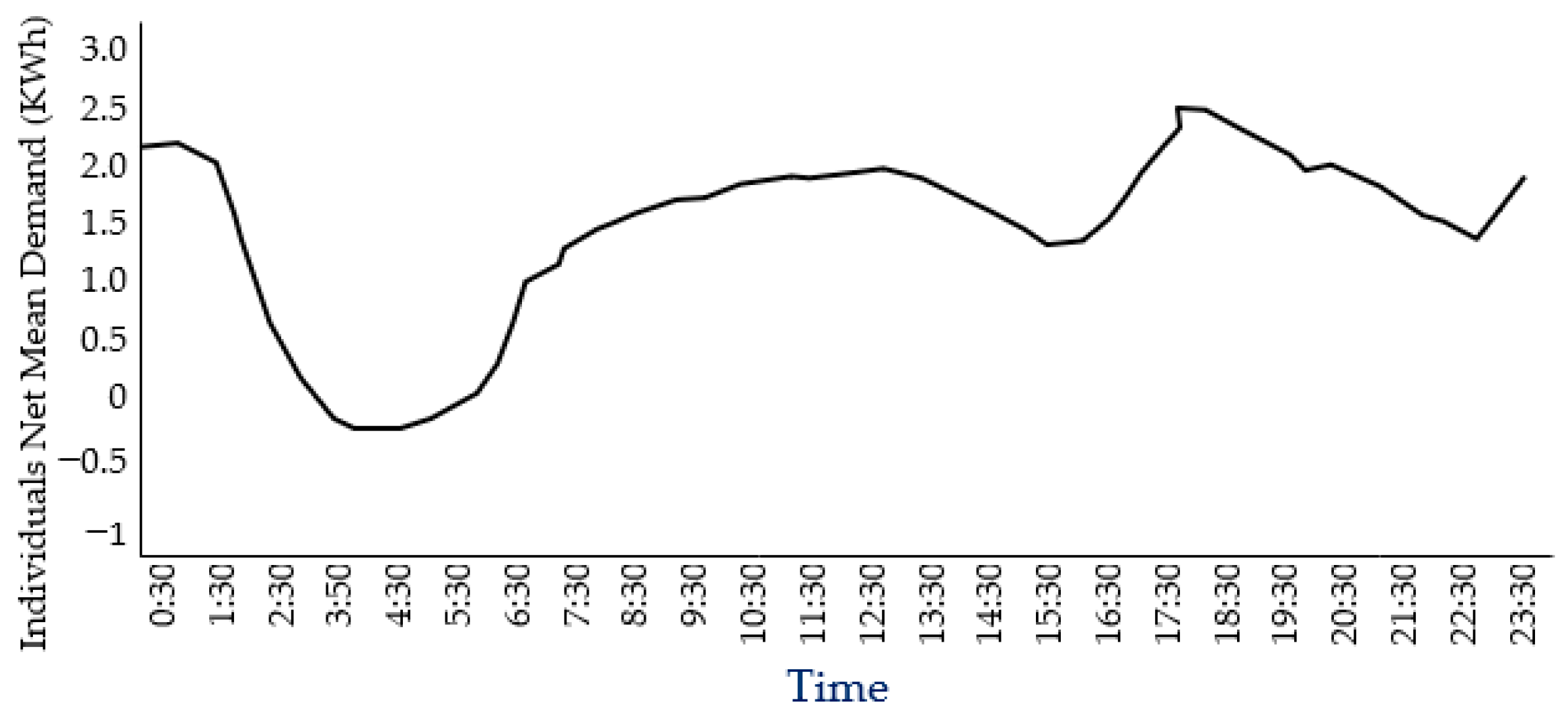
Figure 6.
Tested Sample Weighted index trend chart.

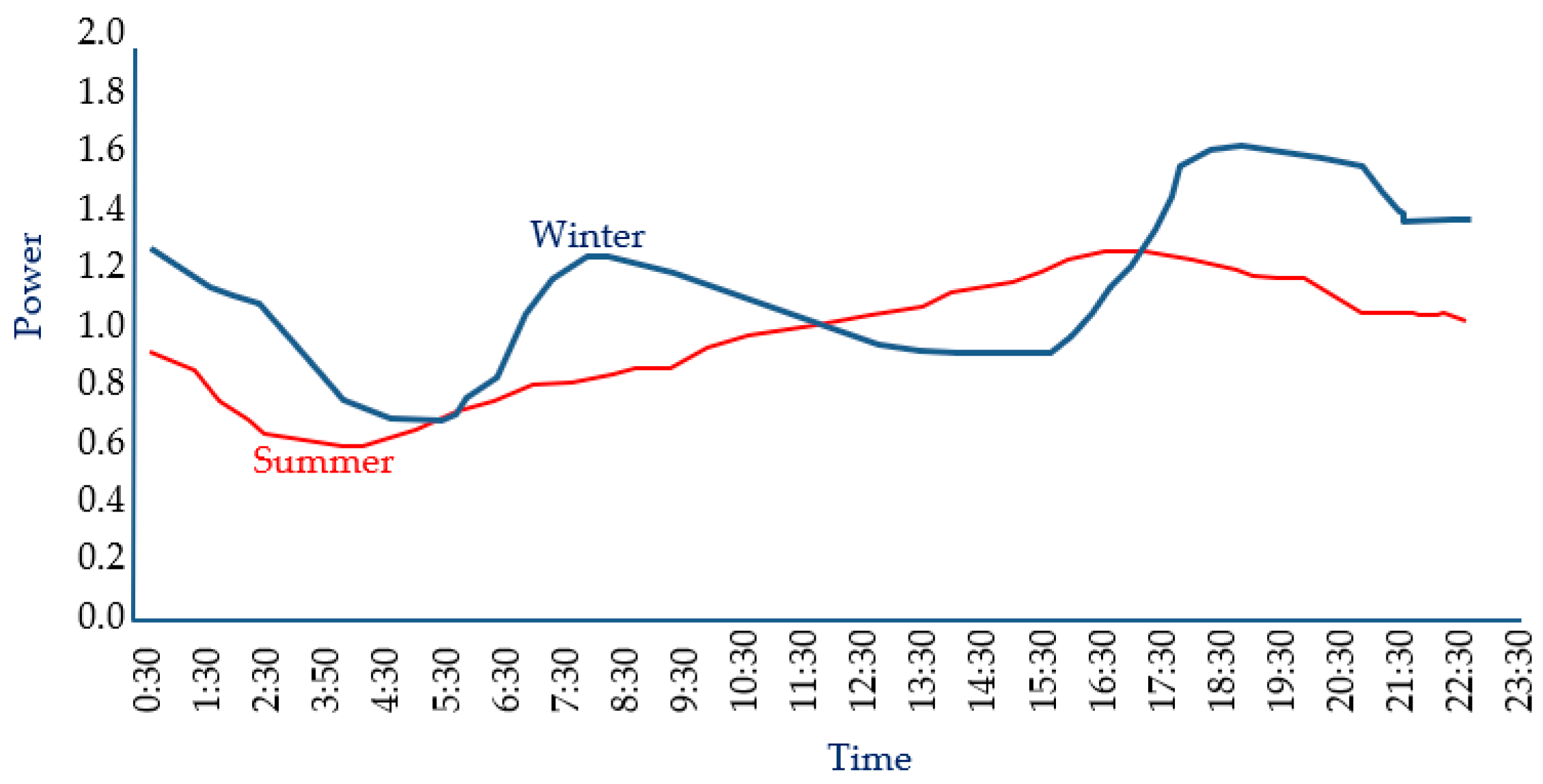
Figure 7.
Australian Houses Typical Average Winter and Summer Demands [44].
Figure 7.
Australian Houses Typical Average Winter and Summer Demands [44].

Figure 8.
Decomposition of time series.

Figure 9.
Dendrogram for time series data.

Figure 10.
Heat map of electricity demand.

Figure 11.
Clusters heterogeneity of electricity demand.

Figure 12.
Average and No Average Events by End-Users.

Figure 13.
Tornado Diagram of Simulation and Optimisation Results.

Figure 14.
Stacked columns of DCAO, DCBO and OG.


Table 1.
Pareto Topolgy.
| Metrics | Formula | Parameters |
|---|---|---|
| Pareto | F(x) = 1 – (k/x) β | X: random variable |
| distribution | K: lower bound of data β: scale parameter shape index data slop |
Table 2.
Sample Size of Residential Houses [46].
Table 2.
Sample Size of Residential Houses [46].
| Metrics | Formula | Parameters | Confidence Level | Population | Sample Size |
|---|---|---|---|---|---|
| Determine Sample Size | Z: Index value of Confidence Level P: Percentage picking a choice expressed as a decimal. C: Confidence interval expressed as decimal | 99% | 2,471,221 | 218 (Residential houses needed for analysis) |
Table 3.
Simulation Analysis of True and False Events by End-Users.
| Time Int. | Max | Min | Mean | Median | 10% Conf | 90% Conf | ui | Avi | li | ui (%) | Avi (%) | li (%) | EUij | (∑li+ui) | (AVi) | (∑li+AVi+ui) | FALSE(%) | TRUE(%) | Total Events(%) |
|---|---|---|---|---|---|---|---|---|---|---|---|---|---|---|---|---|---|---|---|
| 0:30 | 5.94 | 0.00 | 0.47 | 0.17 | 0.71 | 0.08 | 26,156 | 7587 | 72,025 | 24.73% | 7.17% | 68.10% | 100.00% | 98,181 | 7588 | 105,769 | 92.83% | 7.17% | 100.00% |
| 1:00 | 5.87 | 0.00 | 0.46 | 0.16 | 0.69 | 0.07 | 25,185 | 6529 | 74,054 | 23.81% | 6.17% | 70.02% | 100.00% | 99,239 | 6530 | 105,769 | 93.83% | 6.17% | 100.00% |
| 1:30 | 5.58 | 0.00 | 0.43 | 0.15 | 0.68 | 0.07 | 23,311 | 5713 | 76,744 | 22.04% | 5.40% | 72.56% | 100.00% | 100,055 | 5714 | 105,769 | 94.60% | 5.40% | 100.00% |
| 2:00 | 5.32 | 0.00 | 0.35 | 0.14 | 0.66 | 0.07 | 19,367 | 5622 | 80,779 | 18.31% | 5.32% | 76.37% | 100.00% | 100,146 | 5623 | 105,769 | 94.68% | 5.32% | 100.00% |
| 2:30 | 4.63 | 0.00 | 0.29 | 0.14 | 0.60 | 0.07 | 15,914 | 5357 | 84,497 | 15.05% | 5.06% | 79.89% | 100.00% | 100,411 | 5358 | 105,769 | 94.93% | 5.07% | 100.00% |
| 3:00 | 4.27 | 0.00 | 0.24 | 0.13 | 0.66 | 0.07 | 13,137 | 5176 | 87,455 | 12.42% | 4.89% | 82.69% | 100.00% | 100,592 | 5177 | 105,769 | 95.11% | 4.89% | 100.00% |
| 3:30 | 4.27 | 0.00 | 0.22 | 0.13 | 0.59 | 0.07 | 11,958 | 5038 | 88,772 | 11.31% | 4.76% | 83.93% | 100.00% | 100,730 | 5039 | 105,769 | 95.24% | 4.76% | 100.00% |
| 4:00 | 4.25 | 0.00 | 0.21 | 0.13 | 0.65 | 0.07 | 11,483 | 5065 | 89,220 | 10.86% | 4.79% | 84.35% | 100.00% | 100,703 | 5066 | 105,769 | 95.21% | 4.79% | 100.00% |
| 4:30 | 4.31 | 0.00 | 0.21 | 0.13 | 0.61 | 0.07 | 11,151 | 5676 | 88,941 | 10.54% | 5.37% | 84.09% | 100.00% | 100,092 | 5677 | 105,769 | 94.63% | 5.37% | 100.00% |
| 5:00 | 4.32 | 0.00 | 0.21 | 0.13 | 0.25 | 0.37 | 11,579 | 5816 | 88,373 | 10.95% | 5.50% | 83.55% | 100.00% | 99,952 | 5817 | 105,769 | 94.50% | 5.50% | 100.00% |
| 5:30 | 4.16 | 0.00 | 0.23 | 0.13 | 0.09 | 0.21 | 12,766 | 6469 | 86,533 | 12.07% | 6.12% | 81.81% | 100.00% | 99,299 | 6470 | 105,769 | 93.88% | 6.12% | 100.00% |
| 6:00 | 4.22 | 0.00 | 0.25 | 0.14 | 0.04 | 0.49 | 14,253 | 7419 | 84,096 | 13.48% | 7.01% | 79.51% | 100.00% | 98,349 | 7420 | 105,769 | 92.98% | 7.02% | 100.00% |
| 6:30 | 4.85 | 0.00 | 0.29 | 0.15 | 0.09 | 0.21 | 17,072 | 9750 | 78,946 | 16.14% | 9.22% | 74.64% | 100.00% | 96,018 | 9751 | 105,769 | 90.78% | 9.22% | 100.00% |
| 7:00 | 5.32 | 0.00 | 0.35 | 0.18 | 0.06 | 0.27 | 21,781 | 11,701 | 72,286 | 20.59% | 11.06% | 68.34% | 100.00% | 94,067 | 11,702 | 105,769 | 88.94% | 11.06% | 100.00% |
| 7:30 | 5.23 | 0.00 | 0.36 | 0.20 | 0.09 | 0.44 | 22,875 | 14,146 | 68,747 | 21.63% | 13.37% | 65.00% | 100.00% | 91,622 | 14,147 | 105,769 | 86.62% | 13.38% | 100.00% |
| 8:00 | 5.51 | 0.00 | 0.37 | 0.22 | 0.06 | 0.84 | 23,928 | 15,086 | 66,754 | 22.62% | 14.26% | 63.11% | 100.00% | 90,682 | 15,087 | 105,769 | 85.74% | 14.26% | 100.00% |
| 8:30 | 4.90 | 0.00 | 0.36 | 0.22 | 0.08 | 0.23 | 22,959 | 15,604 | 67,205 | 21.71% | 14.75% | 63.54% | 100.00% | 90,164 | 15,605 | 105,769 | 85.25% | 14.75% | 100.00% |
| 9:00 | 5.55 | 0.00 | 0.35 | 0.21 | 0.13 | 0.11 | 22,648 | 14,507 | 68,613 | 21.41% | 13.72% | 64.87% | 100.00% | 91,261 | 14,508 | 105,769 | 86.28% | 13.72% | 100.00% |
| 9:30 | 6.59 | 0.00 | 0.34 | 0.20 | 0.35 | 0.07 | 21,719 | 13,657 | 70,392 | 20.53% | 12.91% | 66.55% | 100.00% | 92,111 | 13,658 | 105,769 | 87.09% | 12.91% | 100.00% |
| 10:00 | 5.25 | 0.00 | 0.33 | 0.19 | 0.16 | 0.08 | 20,725 | 13,086 | 71,957 | 19.59% | 12.37% | 68.03% | 100.00% | 92,682 | 13,087 | 105,769 | 87.63% | 12.37% | 100.00% |
| 10:30 | 5.56 | 0.00 | 0.32 | 0.19 | 0.05 | 0.07 | 20,003 | 12,608 | 73,157 | 18.91% | 11.92% | 69.17% | 100.00% | 93,160 | 12,609 | 105,769 | 88.08% | 11.92% | 100.00% |
| 11:00 | 4.49 | 0.00 | 0.31 | 0.19 | 0.10 | 0.07 | 19,596 | 12,282 | 73,890 | 18.53% | 11.61% | 69.86% | 100.00% | 93,486 | 12,283 | 105,769 | 88.39% | 11.61% | 100.00% |
| 11:30 | 4.76 | 0.00 | 0.31 | 0.19 | 0.06 | 0.07 | 19,445 | 11,988 | 74,335 | 18.38% | 11.33% | 70.28% | 100.00% | 93,780 | 11,989 | 105,769 | 88.66% | 11.34% | 100.00% |
| 12:00 | 5.74 | 0.00 | 0.31 | 0.19 | 0.09 | 0.07 | 19,646 | 12,367 | 73,755 | 18.57% | 11.69% | 69.73% | 100.00% | 93,401 | 12,368 | 105,769 | 88.31% | 11.69% | 100.00% |
| 12:30 | 5.89 | 0.00 | 0.31 | 0.19 | 0.08 | 0.07 | 19,550 | 13,255 | 72,963 | 18.48% | 12.53% | 68.98% | 100.00% | 92,513 | 13,256 | 105,769 | 87.47% | 12.53% | 100.00% |
| 13:00 | 6.22 | 0.00 | 0.31 | 0.19 | 0.06 | 0.07 | 19,149 | 13,466 | 73,153 | 18.10% | 12.73% | 69.16% | 100.00% | 92,302 | 13,467 | 105,769 | 87.27% | 12.73% | 100.00% |
| 13:30 | 4.73 | 0.00 | 0.31 | 0.19 | 0.08 | 0.16 | 18,839 | 13,546 | 73,383 | 17.81% | 12.81% | 69.38% | 100.00% | 92,222 | 13,547 | 105,769 | 87.19% | 12.81% | 100.00% |
| 14:00 | 5.10 | 0.00 | 0.31 | 0.19 | 0.08 | 0.11 | 18,052 | 13,234 | 74,482 | 17.07% | 12.51% | 70.42% | 100.00% | 92,534 | 13,235 | 105,769 | 87.49% | 12.51% | 100.00% |
| 14:30 | 5.63 | 0.00 | 0.30 | 0.19 | 0.34 | 0.08 | 16,950 | 13,363 | 75,455 | 16.03% | 12.63% | 71.34% | 100.00% | 92,405 | 13,364 | 105,769 | 87.36% | 12.64% | 100.00% |
| 15:00 | 5.85 | 0.00 | 0.30 | 0.19 | 0.10 | 0.07 | 16,657 | 13,332 | 75,779 | 15.75% | 12.60% | 71.65% | 100.00% | 92,436 | 13,333 | 105,769 | 87.39% | 12.61% | 100.00% |
| 15:30 | 6.31 | 0.00 | 0.31 | 0.19 | 0.79 | 0.11 | 17,235 | 13,763 | 74,770 | 16.30% | 13.01% | 70.69% | 100.00% | 92,005 | 13,764 | 105,769 | 86.99% | 13.01% | 100.00% |
| 16:00 | 5.80 | 0.00 | 0.32 | 0.20 | 0.34 | 0.25 | 18,416 | 14,555 | 72,797 | 17.41% | 13.76% | 68.83% | 100.00% | 91,213 | 14,556 | 105,769 | 86.24% | 13.76% | 100.00% |
| 16:30 | 6.30 | 0.00 | 0.34 | 0.22 | 0.20 | 0.14 | 20,672 | 15,539 | 69,557 | 19.54% | 14.69% | 65.76% | 100.00% | 90,229 | 15,540 | 105,769 | 85.31% | 14.69% | 100.00% |
| 17:00 | 5.93 | 0.00 | 0.38 | 0.24 | 0.15 | 0.11 | 24,898 | 16,429 | 64,441 | 23.54% | 15.53% | 60.93% | 100.00% | 89,339 | 16,430 | 105,769 | 84.47% | 15.53% | 100.00% |
| 17:30 | 5.40 | 0.00 | 0.45 | 0.28 | 0.19 | 0.11 | 31,454 | 17,200 | 57,114 | 29.74% | 16.26% | 54.00% | 100.00% | 88,568 | 17,201 | 105,769 | 83.74% | 16.26% | 100.00% |
| 18:00 | 5.44 | 0.00 | 0.51 | 0.32 | 0.13 | 0.11 | 37,801 | 18,445 | 49,522 | 35.74% | 17.44% | 46.82% | 100.00% | 87,323 | 18,446 | 105,769 | 82.56% | 17.44% | 100.00% |
| 18:30 | 6.57 | 0.00 | 0.53 | 0.35 | 0.69 | 0.11 | 40,813 | 19,556 | 45,399 | 38.59% | 18.49% | 42.92% | 100.00% | 86,212 | 19,557 | 105,769 | 81.51% | 18.49% | 100.00% |
| 19:00 | 6.34 | 0.00 | 0.53 | 0.36 | 0.15 | 0.11 | 40,767 | 20,896 | 44,105 | 38.54% | 19.76% | 41.70% | 100.00% | 84,872 | 20,897 | 105,769 | 80.24% | 19.76% | 100.00% |
| 19:30 | 6.31 | 0.00 | 0.51 | 0.35 | 0.19 | 0.69 | 39,170 | 22,385 | 44,213 | 37.03% | 21.16% | 41.80% | 100.00% | 83,383 | 22,386 | 105,769 | 78.84% | 21.16% | 100.00% |
| 20:00 | 6.07 | 0.00 | 0.50 | 0.35 | 0.13 | 0.98 | 38,192 | 23,334 | 44,242 | 36.11% | 22.06% | 41.83% | 100.00% | 82,434 | 23,335 | 105,769 | 77.94% | 22.06% | 100.00% |
| 20:30 | 5.69 | 0.00 | 0.50 | 0.35 | 0.15 | 0.50 | 38,403 | 23,804 | 43,561 | 36.31% | 22.51% | 41.19% | 100.00% | 81,964 | 23,805 | 105,769 | 77.49% | 22.51% | 100.00% |
| 21:00 | 5.59 | 0.00 | 0.48 | 0.34 | 0.31 | 0.40 | 36,352 | 24,129 | 45,287 | 34.37% | 22.81% | 42.82% | 100.00% | 81,639 | 24,130 | 105,769 | 77.19% | 22.81% | 100.00% |
| 21:30 | 5.46 | 0.00 | 0.45 | 0.32 | 0.33 | 0.39 | 33,508 | 23,530 | 48,730 | 31.68% | 22.25% | 46.07% | 100.00% | 82,238 | 23,531 | 105,769 | 77.75% | 22.25% | 100.00% |
| 22:00 | 6.52 | 0.00 | 0.44 | 0.30 | 0.19 | 0.38 | 31,186 | 21,054 | 53,528 | 29.49% | 19.91% | 50.61% | 100.00% | 84,714 | 21,055 | 105,769 | 80.09% | 19.91% | 100.00% |
| 22:30 | 6.34 | 0.00 | 0.44 | 0.27 | 0.69 | 0.26 | 30,254 | 17,857 | 57,657 | 28.60% | 16.88% | 54.51% | 100.00% | 87,911 | 17,858 | 105,769 | 83.12% | 16.88% | 100.00% |
| 23:00 | 6.54 | 0.00 | 0.42 | 0.23 | 0.54 | 0.06 | 27,480 | 14,707 | 63,581 | 25.98% | 13.90% | 60.11% | 100.00% | 91,061 | 14,708 | 105,769 | 86.09% | 13.91% | 100.00% |
| 23:30 | 6.41 | 0.00 | 0.43 | 0.21 | 0.89 | 0.08 | 26,744 | 12,120 | 66,904 | 25.29% | 11.46% | 63.26% | 100.00% | 93,648 | 12,121 | 105,769 | 88.54% | 11.46% | 100.00% |
| 0:00 | 5.59 | 0.00 | 0.46 | 0.19 | 1.19 | 0.07 | 26,608 | 9727 | 69,433 | 25.16% | 9.20% | 65.65% | 100.00% | 96,041 | 9728 | 105,769 | 90.80% | 9.20% | 100.00% |
Table 4.
Data Simulation and Optimisation Analysis.
| Population-Id | Demand Unit | ||||||||
|---|---|---|---|---|---|---|---|---|---|
| (l + u)-False | AV-True | l-False | u-False | AV-True | Under-Demand | Over-Demand | Optimum | ||
| 1 Tier | 44 | 4 | 23 | 0 | 25 | −0.4792 | 0.0000 | 0.5208 | 0.4792 |
| 2 Tier | 43 | 5 | 32 | 15 | 1 | −0.6667 | 0.3125 | 0.0208 | 0.9792 |
| 3 Tier | 44 | 4 | 23 | 5 | 20 | −0.4792 | 0.1042 | 0.4167 | 0.5833 |
| 4 Tier | 43 | 5 | 12 | 0 | 36 | −0.2500 | 0.0000 | 0.7500 | 0.2500 |
| 5 Tier | 46 | 4 | 31 | 8 | 9 | −0.6458 | 0.1667 | 0.1875 | 0.8125 |
| 6 Tier | 41 | 7 | 4 | 0 | 44 | −0.0833 | 0.0000 | 0.9167 | 0.0833 |
| 7 Tier | 40 | 8 | 3 | 0 | 45 | −0.0625 | 0.0000 | 0.9375 | 0.0625 |
| 8 Tier | 42 | 6 | 6 | 0 | 42 | −0.1250 | 0.0000 | 0.8750 | 0.1250 |
| 9 Tier | 43 | 5 | 0 | 0 | 48 | 0.0000 | 0.0000 | 1.0000 | 0.0000 |
| 10 Tier | 40 | 8 | 7 | 1 | 40 | −0.1458 | 0.0208 | 0.8333 | 0.1667 |
| 11 Tier | 41 | 7 | 12 | 5 | 31 | −0.2500 | 0.1042 | 0.6458 | 0.3542 |
| 12 Tier | 43 | 5 | 22 | 0 | 26 | −0.4583 | 0.0000 | 0.5417 | 0.4583 |
| 13 Tier | 41 | 7 | 4 | 3 | 41 | −0.0833 | 0.0625 | 0.8542 | 0.1458 |
| 14 Tier | 42 | 6 | 8 | 0 | 40 | −0.1667 | 0.0000 | 0.8333 | 0.1667 |
| 15 Tier | 44 | 4 | 9 | 0 | 39 | −0.1875 | 0.0000 | 0.8125 | 0.1875 |
| 16 Tier | 43 | 5 | 13 | 0 | 35 | −0.2708 | 0.0000 | 0.7292 | 0.2708 |
| 17 Tier | 44 | 4 | 27 | 0 | 21 | −0.5625 | 0.0000 | 0.4375 | 0.5625 |
| 18 Tier | 43 | 5 | 40 | 8 | 0 | −0.8333 | 0.1667 | 0.0000 | 1.0000 |
| 19 Tier | 42 | 6 | 13 | 4 | 31 | −0.2708 | 0.0833 | 0.6458 | 0.3542 |
| 20 Tier | 43 | 5 | 19 | 29 | 0 | −0.3958 | 0.6042 | 0.0000 | 1.0000 |
| 21 Tier | 43 | 5 | 0 | 0 | 48 | 0.0000 | 0.0000 | 1.0000 | 0.0000 |
| 22 Tier | 44 | 4 | 24 | 10 | 14 | −0.5000 | 0.2083 | 0.2917 | 0.7083 |
| 23 Tier | 43 | 5 | 11 | 0 | 37 | −0.2292 | 0.0000 | 0.7708 | 0.2292 |
| 24 Tier | 44 | 4 | 25 | 0 | 23 | −0.5208 | 0.0000 | 0.4792 | 0.5208 |
| 25 Tier | 41 | 7 | 1 | 0 | 47 | −0.0208 | 0.0000 | 0.9792 | 0.0208 |
| 26 Tier | 45 | 3 | 32 | 0 | 16 | −0.6667 | 0.0000 | 0.3333 | 0.6667 |
| 27 Tier | 44 | 4 | 17 | 0 | 31 | −0.3542 | 0.0000 | 0.6458 | 0.3542 |
| 28 Tier | 44 | 4 | 7 | 1 | 40 | −0.1458 | 0.0208 | 0.8333 | 0.1667 |
| 29 Tier | 43 | 5 | 8 | 1 | 39 | −0.1667 | 0.0208 | 0.8125 | 0.1875 |
Table 5.
Summary of Data Simulation and Optimisation Analysis.
| Percentile Demand Rate | False-Demand (%) | True-Demand (%) |
|---|---|---|
| Optimisation (%) | 56.54% | 43.46% |
| Simulation (%) | 89.30% | 10.70% |
| Total Population | 290 | 290 |
Table 6.
Load Capacity Factor for Coal & Gas Generators Vs. Cost $/MWh.
| Optimal Capacity Factor for Generators Associated with Entry Cost $/MWh. | |||
|---|---|---|---|
| Load Factor (CF) | 100% | 55% | 14% |
| Thermal Coal-CP | $36.2 MWh | Higher than $55.9 MWh | Higher than $109.0 MWh |
| CCGT | Higher than $36.2 MWh | $55.9MWh | Higher than $109.0 MWh |
| OCGT | Higher than $36.2 MWh | Higher than $55.9 MWh | $109.0MWh |
Table 7.
Comparing Losses Cost of Simulation and Optimisation.
| Demand Cost Benefit(₵) | |||||
|---|---|---|---|---|---|
| Tiers | Simulation Modelling | Optimisation Modelling | |||
| DCBO(₵) | Losses(%) | DCAO(₵) | Gains (%) | OG(₵) | |
| 1T | 1268.37 | 0.4149 | 526.24 | 0.5851 | 742.13 |
| 2T | 970.15 | 0.2900 | 281.34 | 0.7100 | 688.81 |
| 3T | 1156.29 | 0.3191 | 368.98 | 0.6809 | 787.31 |
| 4T | 1083.83 | 0.3968 | 430.07 | 0.6032 | 653.75 |
| 5T | 1077.13 | 0.3266 | 351.78 | 0.6734 | 725.34 |
| 6T | 943.93 | 0.4854 | 458.20 | 0.5146 | 485.74 |
| 7T | 852.32 | 0.4690 | 399.71 | 0.5310 | 452.60 |
| 8T | 999.49 | 0.3761 | 375.89 | 0.6239 | 623.60 |
| 9T | 1282.73 | 0.1167 | 149.64 | 0.8833 | 1133.09 |
| 10T | 1079.53 | 0.5443 | 587.59 | 0.4557 | 491.94 |
| 11T | 1049.83 | 0.4137 | 434.35 | 0.5863 | 615.47 |
| 12T | 1160.90 | 0.3669 | 425.88 | 0.6331 | 735.02 |
| 13T | 1079.98 | 0.5001 | 540.06 | 0.4999 | 539.92 |
| 14T | 1340.14 | 0.3676 | 492.64 | 0.6324 | 847.50 |
| 15T | 1532.55 | 0.3711 | 568.79 | 0.6289 | 963.76 |
| 16T | 1424.33 | 0.3902 | 555.81 | 0.6098 | 868.52 |
| 17T | 977.42 | 0.3381 | 330.47 | 0.6619 | 646.95 |
| 18T | 1164.67 | 0.3529 | 410.99 | 0.6471 | 753.68 |
| 19T | 1026.28 | 0.4496 | 461.42 | 0.5504 | 564.86 |
| 20T | 918.47 | 0.2900 | 266.36 | 0.7100 | 652.12 |
| 21T | 838.67 | 0.3905 | 327.53 | 0.6095 | 511.14 |
| 22T | 1348.01 | 0.3541 | 477.39 | 0.6459 | 870.63 |
| 23T | 987.16 | 0.4173 | 411.93 | 0.5827 | 575.23 |
| 24T | 883.66 | 0.3835 | 338.86 | 0.6165 | 544.80 |
| 25T | 1005.46 | 0.3900 | 392.13 | 0.6100 | 613.33 |
| 26T | 1287.68 | 0.3151 | 405.78 | 0.6849 | 881.90 |
| 27T | 1122.55 | 0.4017 | 450.95 | 0.5983 | 671.60 |
| 28T | 1147.01 | 0.4270 | 489.80 | 0.5730 | 657.20 |
| 29T | 1523.30 | 0.3974 | 605.33 | 0.6026 | 917.97 |
Table 8.
Summarising Losses Cost of Comparison.
| Energy Losses | Cost of Losses (¢) | Cost of Gains (¢) | Impact (%) | |
|---|---|---|---|---|
| Simulation | DCBO | (32,531.83) | −(100%) | |
| Optimisation | DCAO | (12,315.92) | −(37.86%) | |
| OG | 20,215.90 | +(62.14%) | ||
Table 9.
Losses Cost Simulation and Optimisation.
| Population-id | Electricity Supply (KWh) (GC + CL) | Constraints (End-Users Demand) | Expected Power Constraints at Homes | |||
|---|---|---|---|---|---|---|
| Fault 1 | Fault 2 | |||||
| Available Stock | Optimisation Results | Under Demand | Over Demand | GG2 | GG1 | |
| 1TIER | 175.61 | 183.59 | −7.98 | 0.00 | 1 | 2 |
| 2TIER | 163.84 | 181.67 | −44.61 | 26.78 | 2 | 2 |
| 3TIER | 147.95 | 158.14 | −12.12 | 1.93 | 2 | 2 |
| 4TIER | 167.00 | 176.27 | −9.27 | 0.00 | 1 | 2 |
| 5TIER | 134.00 | 152.08 | −20.33 | 2.25 | 2 | 2 |
| 6TIER | 221.62 | 222.96 | −1.34 | 0.00 | 1 | 2 |
| 7TIER | 193.55 | 194.43 | −0.88 | 0.00 | 1 | 2 |
| 8TIER | 174.27 | 177.06 | −2.79 | 0.00 | 1 | 2 |
| 9TIER | 154.14 | 154.14 | 0.00 | 0.00 | 1 | 1 |
| 10TIER | 211.7 | 215.94 | −4.24 | 0.00 | 1 | 2 |
| 11TIER | 175.33 | 178.44 | −9.09 | 5.98 | 1 | 2 |
| 12TIER | 147.18 | 163.18 | −16.00 | 0.00 | 1 | 2 |
| 13TIER | 210.15 | 210.82 | −0.67 | 0.00 | 1 | 2 |
| 14TIER | 172.79 | 174.00 | −1.21 | 0.00 | 1 | 2 |
| 15TIER | 171.62 | 177.50 | −5.88 | 0.00 | 1 | 2 |
| 16TIER | 177.61 | 184.74 | −7.13 | 0.00 | 1 | 2 |
| 17TIER | 140.74 | 157.99 | −17.25 | 0.00 | 1 | 2 |
| 18TIER | 140.74 | 158.11 | −26.12 | 8.75 | 2 | 2 |
| 19TIER | 185.23 | 188.98 | −4.96 | 1.21 | 2 | 2 |
| 20TIER | 166.33 | 139.20 | −7.54 | 34.67 | 2 | 2 |
| 21TIER | 166.71 | 166.71 | 0.00 | 0.00 | 1 | 1 |
| 22TIER | 157.00 | 169.41 | −15.09 | 2.68 | 2 | 2 |
| 23TIER | 170.03 | 177.38 | −7.35 | 0.00 | 1 | 2 |
| 24TIER | 155.34 | 165.00 | −9.66 | 0.00 | 1 | 2 |
| 25TIER | 234.99 | 234.99 | 0.00 | 0.00 | 1 | 1 |
| 26TIER | 130.53 | 149.24 | −18.71 | 0.00 | 1 | 2 |
| 27TIER | 168.53 | 177.18 | −8.65 | 0.00 | 1 | 2 |
| 28TIER | 189.57 | 192.28 | −2.71 | 0.00 | 1 | 2 |
| 29TIER | 179.23 | 185.73 | −6.50 | 0.00 | 1 | 2 |
Table 10.
Summarising Losses Cost Simulation and Optimisation.
| Capacity | Impact Factor | Expected Power Sources | |
|---|---|---|---|
| Under Demand Constraints | 268.08 | 89.65% | GG1 |
| Over Demand Constraints | 84.25 | 24.13% | GG2 |
| Total Available Stock | 4983.33 | 89.65% | (GC+CL) |
| Total Optimisation Results | 5167.16 | 100.00% | Mix |
Table 11.
Z Test.
| Z-Test: One Sample | x1 | x2 | x3 | x4 | x5 | x6 | x7 | x8 | x9 | x10 | x11 | x12 | x13 | x14 | x15 | x16 | x17 | x18 |
|---|---|---|---|---|---|---|---|---|---|---|---|---|---|---|---|---|---|---|
| Mean | 0.357 | 0.357 | 0.357 | 0.357 | 0.357 | 0.357 | 0.357 | 0.357 | 0.357 | 0.357 | 0.357 | 0.357 | 0.357 | 0.357 | 0.357 | 0.357 | 0.357 | 0.357 |
| Known Variance | 0.008 | 0.008 | 0.008 | 0.008 | 0.008 | 0.008 | 0.008 | 0.008 | 0.008 | 0.008 | 0.008 | 0.008 | 0.008 | 0.008 | 0.008 | 0.008 | 0.008 | 0.008 |
| Observations | 48 | 48 | 48 | 48 | 48 | 48 | 48 | 48 | 48 | 48 | 48 | 48 | 48 | 48 | 48 | 48 | 48 | 48 |
| Hypothesized Mean | 0.29 | 0.30 | 0.31 | 0.32 | 0.33 | 0.34 | 0.35 | 0.36 | 0.37 | 0.38 | 0.39 | 0.40 | 0.41 | 0.42 | 0.43 | 0.44 | 0.45 | 0.46 |
| z | 5.03 | 4.284 | 3.539 | 2.794 | 2.048 | 1.303 | 0.558 | −0.19 | −0.93 | −1.68 | −2.42 | −3.17 | −3.91 | −4.66 | −5.4 | −6.15 | −6.89 | −7.64 |
| P(Z ≤ z) two-tail | 5 × 10⁻⁷ | 2 × 10⁻⁵ | 4 × 10⁻⁴ | 0.005 | 0.041 | 0.193 | 0.577 | 0.851 | 0.351 | 0.093 | 0.015 | 0.002 | 9 × 10⁻⁵ | 3 × 10⁻⁶ | 7 × 10⁻⁸ | 8 × 10⁻¹⁰ | 5 × 10⁻¹² | 2 × 10⁻¹⁴ |
| z Critical two-tail | 2.576 | 2.576 | 2.576 | 2.576 | 2.576 | 2.576 | 2.576 | 2.576 | 2.576 | 2.576 | 2.576 | 2.576 | 2.576 | 2.576 | 2.576 | 2.576 | 2.576 | 2.576 |
| p-value | <0.001 | <0.001 | <0.001 | <0.001 | >0.001 | >0.001 | >0.001 | >0.001 | >0.001 | >0.001 | >0.001 | >0.001 | <0.001 | <0.001 | <0.001 | <0.001 | <0.001 | <0.001 |
Publisher’s Note: MDPI stays neutral with regard to jurisdictional claims in published maps and institutional affiliations. |
© 2021 by the authors. Licensee MDPI, Basel, Switzerland. This article is an open access article distributed under the terms and conditions of the Creative Commons Attribution (CC BY) license (http://creativecommons.org/licenses/by/4.0/).
Share and Cite
MDPI and ACS Style
Zaghwan, A.; Gunawan, I. Resolving Energy Losses Caused by End-Users in Electrical Grid Systems. Designs 2021, 5, 23. https://0-doi-org.brum.beds.ac.uk/10.3390/designs5010023
AMA Style
Zaghwan A, Gunawan I. Resolving Energy Losses Caused by End-Users in Electrical Grid Systems. Designs. 2021; 5(1):23. https://0-doi-org.brum.beds.ac.uk/10.3390/designs5010023
Chicago/Turabian StyleZaghwan, Ashraf, and Indra Gunawan. 2021. "Resolving Energy Losses Caused by End-Users in Electrical Grid Systems" Designs 5, no. 1: 23. https://0-doi-org.brum.beds.ac.uk/10.3390/designs5010023