TomoSim: A Tomographic Simulator for Differential Optical Absorption Spectroscopy


1
Physics Department, FCT NOVA, NOVA University of Lisbon, 2829-516 Caparica, Portugal
2
FutureCompta SA, 1495-190 Algés, Portugal
3
Biomedical Engineering and Biophysics Institute, University of Lisbon, 1749-016 Lisbon, Portugal
*
Author to whom correspondence should be addressed.
Drones 2021, 5(1), 3; https://0-doi-org.brum.beds.ac.uk/10.3390/drones5010003
Submission received: 13 November 2020
/
Revised: 19 December 2020
/
Accepted: 21 December 2020
/
Published: 29 December 2020
Abstract
:TomoSim comes as part of project ATMOS, a miniaturised Differential Optical Absorption Spectroscopy (DOAS) tomographic atmospheric evaluation device, designed to fit a small drone. During the development of the project, it became necessary to write a simulation tool for system validation. TomoSim is the answer to this problem. The software has two main goals: to mathematically validate the tomographic acquisition method; and to allow some adjustments to the system before reaching final product stages. This measurement strategy was based on a drone performing a sequential trajectory and gathering projections arranged in fan beams, before using some classical tomographic methods to reconstruct a spectral image. The team tested three different reconstruction algorithms, all of which were able to produce an image, validating the team’s initial assumptions regarding the trajectory and acquisition strategy. All algorithms were assessed on their computational performance and their ability for reconstructing spectral “images”, using two phantoms, one of which custom made for this purpose. In the end, the team was also able to uncover certain limitations of the TomoSim approach that should be addressed before the final stages of the system.
1. Introduction
1.1. Background and Motivation
This article details the construction of TomoSim, which is the software simulation package used in the ATMOS project, a Portuguese European Union (EU) funded initiative that aimed at creating a miniaturised spectroscopy platform for atmospheric monitoring and trace gas mapping. The project was a joint effort from Compta, S.A., one of the oldest IT groups in Portugal; and FCT NOVA, from the NOVA University of Lisbon, also one of the largest and most important science schools in the country.
The idea of using a tomographically capable drone with spectroscopic equipment for mapping trace gas concentrations in defined geographical regions made the need for a simulation tool evident from a very early stage. Any monitoring device that depends on drones for the actual measurements must take into account a number of restrictions, of both physical and logistical order (weight, battery life, etc.). These considerations are even more important if the measurements themselves depend on the ability of the drone to move and position itself a certain way and the precision with which it can do so. For the ATMOS project, they were paramount. Simulation is a simple and inexpensive way of determining the technical feasibility of the project and the mathematical validity of the reconstruction strategy.
This strategy is based on two premises:
- A custom-equipped drone should be able to measure trace gas column density in a carefully programmed sequence;
- One can then organise these measurements into an array.
These column density values could then be used as projections in a tomographic reconstruction. The resulting image would correspond to the geographic distribution of the target trace gases.
The simulator, built in Python [1] and using NumPy [2], uses the system’s premise and applies three algorithms for reconstruction: fan beam Filtered BackProjection (FBP), Simultaneous algebraic Reconstruction Technique (SART) and Maximum Likelihood Expectation Maximisation (MLEM). Algorithm verification and analysis was performed using a custom-designed phantom for DOAS spectral measurements.All three mathematical algorithms managed to reconstruct the image. FBP was shown to be significantly more computationally cost-effective than the other two. The custom coded MLEM routine was not on-par with the other two solutions, which were plugged directly from the SciPy library.
Besides runtime and other significant software engineering considerations, the development of TomoSim concluded that the assumptions of the team regarding the acquisition strategy for spectral geographic images were correct, but lifted the veil on some limitations that should be addressed before building the final system.
The paper is structured as follows: the section after this introduction, Section 1, targets the theoretical background with which the paper was built; Section 2 describes the design, the rationale behind it and the technical choices that have been taken in the making of TomoSim; in Section 3 there is a description of the results that were obtained through the simulator, including reconstructions, running times and Section 5 is dedicated to the conclusions that were taken using this piece of software, as well as some foreseeable future developments.
1.2. Differential Optical Absorption Spectroscopy (DOAS)
DOAS is a widely used atmospheric analysis technique, developed in the late 1960s. Fundamentally, it is an absorption spectroscopy technique, therefore based on Lambert-Beer’s law. This law was actually first formulated by Pierre Bouguer in 1729. At the time, he wrote that “in a medium of uniform transparency, the light remaining in a collimated beam is an exponential function of the length of the path in the medium” [3]. This theory can thus be written as in Equation (1).
is the source intensity of a light beam, the intensity of the light that reaches the detector, is the absorption cross-section of the chemical compound being measured, c its concentration and L the optical path of the light (the length of the path that is traversed by the ray of light). Finally, is the wavelength of the radiation.
The rearrangement of Equation (1) gives us the concentration, and more importantly, allows us the creation of a new quantity, , which is called optical depth. This is explicit in Equation (2) [4,5].
In the laboratory, this equation can be (and is) used directly and with few obstacles, since there are very few uncontrolled variables, and that which exists is controlled for. In the open atmosphere, this is not the case at all.
There are many factors that influence the degree to which we can apply Lambert-Beer’s rule in atmospheric measurements. The most important one is the fact that in order to know the source intensity (), one would have to remove any and every absorber from optical path, and this is clearly infeasible in the great majority of circumstances. To surpass this problem, DOAS measures differences between absorption structures at many different wavelengths [5].
There are many different DOAS systems, but the single greatest distinction among them is whether they are active or passive. Active systems use artificial light sources such as a Xenon lamp to measure chemicals in the air. Passive systems use natural sources, such as the Sun or the Moon (or other celestial bodies). This paper will focus on passive systems, since the ATMOS project is a scattered sunlight DOAS system, and thus passive.
Scattered sunlight DOAS systems have their own specific particularities and special properties. For instance, the optical path is unknown as the last scattering event cannot be determined. Scattering also implies that there is a fraction of the source’s light that does not reach the detector. Moreover, one must account for all the other passive DOAS common effects, such as the fact that there are many absorbers that have spectral structures overlapping the target species; that there are Fraunhofer lines, Mie and Rayleigh scattering, turbulence and instrumental effects, and so forth [5,6].
All these influential effects mean that, in the open atmosphere, Equation (3) is a more plausible model than that presented in Equation (1).
In Equation (3), there is more than one absorber, which is denoted by index i in the sum. denotes the fraction of light that gets scattered into the detector, and are Mie and Rayleigh scattering coefficients, and the integral is performed on the whole optical path, s.
Typically, we measure a trace gas’s atmospheric contribution by its total column. This quantity is essentially the integral of the compound’s number density, in molecules/cm3, over a column that goes from the ground to the Top Of the Atmosphere (TOA). In Equation (4), the number density for molecule x is denoted .
One can look again at Equation (3) with the interest of quantifying only the trace gas contribution. This contribution should be somehow related to the total column, since the only real difference between what the DOAS instruments see and the total column is the dependence on the optical path of the former. In fact, we can separate the integral to get the trace absorbers optical density expression, displayed in Equation (5). Since we can consider the cross-section to be fairly constant with the optical path, it is possible to separate this integral, and we arrive at the very important value of the slant column, , which is the integral of the gas’s number density along the optical path.
If we integrate the absorption coefficients inside the exponential term of Equation (3) to their optical densities, we arrive at the expression in Equation (6). This equation cannot be solved without some very seldomly available data, such as the original light source . DOAS allows us to overcome this problem by making relative measurements (hence the differential in the name of the technique), using another scattered light spectrum as reference and by observing that most interesting trace gases have very narrow spectral structures, while effects like Mie and Rayleigh scattering have broad spectral features.
and are, respectively, the reference light intensity and reference scattered light ratio and and the integrated optical depth of the Rayleigh and Mie scattering phenomena. It is thus possible to separate the original optical depth in two parts, a differential part, which is comprised of the narrowband contributions coming mainly from trace gases; and the “continuous” part, which contains the slow-variation, broadband contributions in Equation (3). The latter can be approximated by fitting a low order polynomial to the original optical depth signal. If one subtracts this polynomial from the optical depth, the result is the narrowband signal that constitutes the differential part. Target absorbers column densities can then be found by fitting their cross-sections to the differential signal, using a numerical algorithm such as Levenberg-Marquardt’s [7].
1.3. The Tomography Problem
1.3.1. Introduction
Tomography is the cross-sectional imaging of an object through the use of transmitted or reflected waves, collected by the object exposure to the waves from a set of known angles. Tomography has many different applications in science, industry, and in particular, medicine. Since the invention of the Computed Tomography (CT) machine, in 1972 by Hounsfield [8], tomographic imaging techniques have had a revolutionary impact, allowing doctors to see inside their patients without having to subject them to surgical interventions. Examples of tomographic applications for scientific and industrial purposes include radio-astronomy and certain kinds of tomographic non-destructive test techniques [9].
Tomography has had its mathematical basis set by Johannes Radon, a German mathematician that proved that it is possible to represent a function in (the domain of the real numbers) in the space of straight lines through its line integrals. In the tomographic case, these integrals represent a measurement on a ray that is traversing the field of analysis. Each set of line integrals (rays), characterised by a given projection angle, is called a projection. The set of all projections, arranged in matrix form by projection angle and detector is called a sinogram. All reconstruction methods revolve around this matrix [9,10,11].
1.3.2. Discretisation
Siddon’s algorithm [12], published in 1985, is one of the most common and most studied ways to go from the naturally analogical presentation of the real world into computer-operable discrete geometric fields of vectors, in the field of tomography. The algorithm considers each pixel to be the intersection area of orthogonal sets of equally spaced parallel planes. With this in mind, it is possible to parametrise a ray of light, with the ray being written (in two dimensions):
In Equation (7), and are the coordinates for the entry point (of the ray in the analysis field) and and are the exit point coordinates. is the parametric value. If the ray is totally contained within the field of analysis, this value varies between 0 and 1; otherwise, it has its minimum at the entry point and maximum at the exit.
The parametrical representation of the line integral, allows one to recursively calculate all intersections between the ray and the grid defined by the orthogonal lines described above. The differences between intersection points render the lengths of each ray contained within each pixel. The sum of all the lengths for one ray yields the total value of the line integral, which corresponds to a projection. The algorithm steps are presented in Algorithm 1 [12,13].
| Algorithm 1: Siddon’s algorithm’s procedural steps. After running this algorithm, one is able to represent any continuous ray through the analysis field as a sum of discrete lengths |
| Result: Discretised Region of Interest(ROI). calculate range of parametric values; calculate range of pixel indices; calculate parametric sets; merge sets; calculate pixel(or voxel) lengths; calculate pixel indices; |
1.3.3. Geometry
The application of analytical algorithms such as FBP depends on the type of geometric arrangement of the tomographic problem. TomoSim uses two tomographic geometries in its reconstructions: parallel and fan beam.
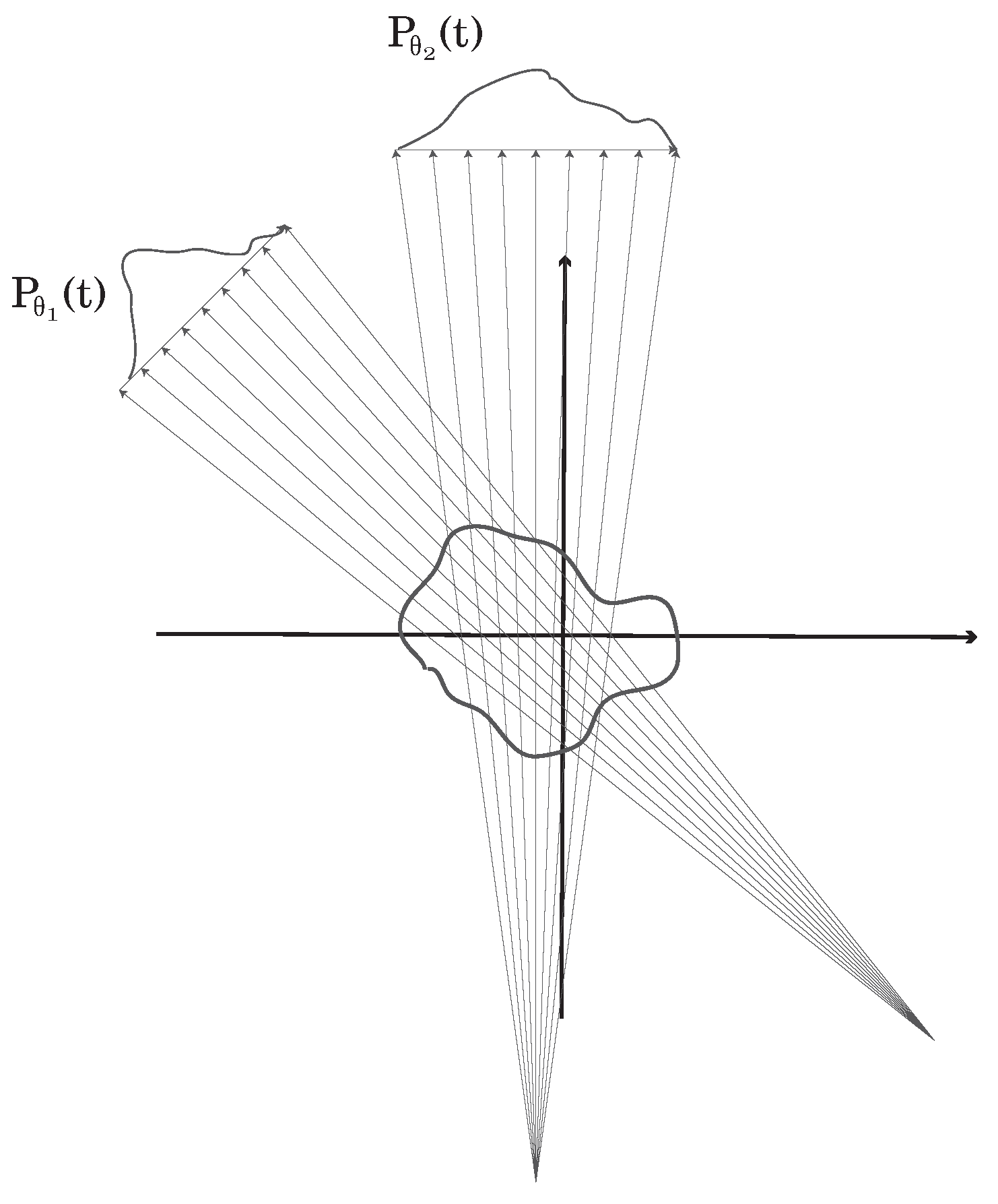
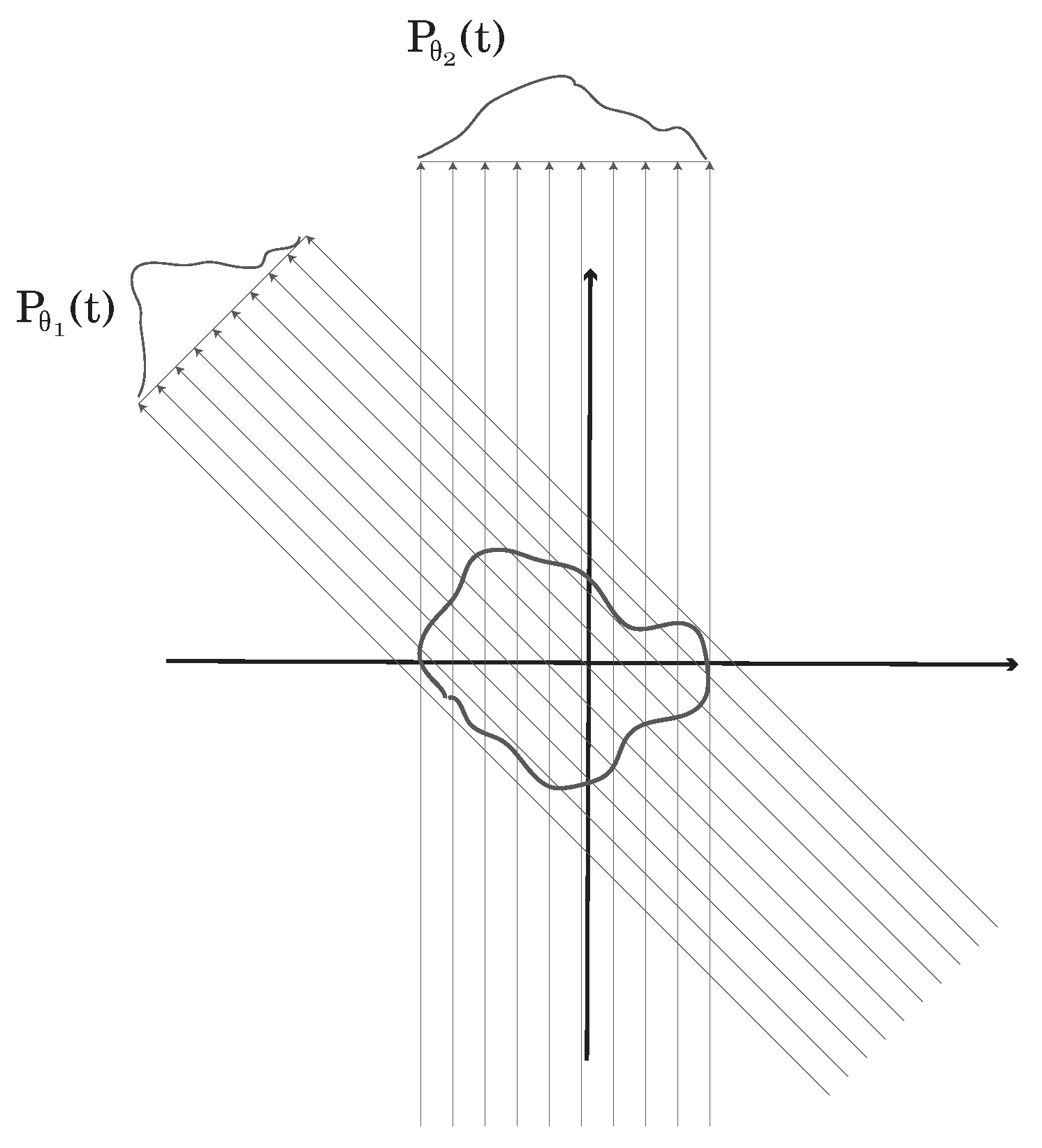
Parallel Projection geometry (see Figure 1) is the most basic assembly. In this arrangement, each projection is a set of parallel line integrals, as can be seen in Figure 1. The radiation sources can be assembled in a linear array, facing detectors in the same number on the opposite side of the target object, or, in alternative, a single source can move in a linear trajectory, directing its rays onto an array of detectors, linearly arranged on the opposite side of the target object. Projections of this sort are characterised by the projection angle, which is the angle each ray makes with the vertical axis. The other relevant geometric assembly is the fan beam arrangement (see Figure 1). In this projection mode, all radiation in the projection comes from a single source, with rays being directed outwards onto a set of detectors, which may be arranged on a circumference arc (equiangular rays) or on a straight line (equally spaced rays) [9].
1.3.4. Reconstruction
The overarching division between tomographic reconstruction algorithms is on the level of their nature, which can be analytical or algebraic (iterative). Other subdivisions come from the geometry and the type of technology used for the particular application on which reconstruction is being run. In medical imaging, the most common analytical method is the Filtered BackProjection algorithm (FBP). FBP is based on Fourier’s Slice Theorem, which states that the one dimensional Fourier Transform (FT) of a projection at a given angle is the two dimensional FT of the reconstructed image through that same angle [9,14]. If a sufficient number of projections is gathered, one can create a good estimate of the image by performing a 1D FT of the projections, and inverting them in 2D, before summing them in the image space. It so happens that this direct inversion process produces heavily distorted images due to the fact that calculation errors are typically larger the higher the frequency of the image component [9]. This is overcome in FBP by the application of a weighing filter before the inversion process.
This sequence of steps is sufficient for parallel projection reconstruction, but for fan beam projections, the FBP can only be applied after a series of somewhat cumbersome geometric transformations. If this is not acceptable, for some reason, there is an alternate solution: the fan beam sinogram can be reorganised, based on the observation that a ray in a fan beam is equal to a ray in a parallel projection in another given angle. Of course this resorting operation will not render a perfect sinogram for this new parallel projection (since not every fan ray has a direct parallel ray correspondent), but imperfections can be normally corrected through interpolation. After this procedure is run, one can proceed as if the geometry were parallel [9,11,15].
Iterative algorithms are based on simpler premises, but require a different mindset. The set of projections can be thought of as a matrix, called sinogram, as has been introduced in this same section. In this matrix, the lines refer to the projection number, and the columns deal with the detectors (for instance, the first line of this matrix corresponds to all detections in the first projection). The image can also be thought of as a matrix, in which each pixel has a given value, which gives it its intensity (and/or colour). Finally, there is the system matrix, which is the matrix that contains the lengths of every ray in each projection contained in each one of the image’s pixels, lengths which are obtained, in this case, through Siddon’s algorithm, already presented. Iterative algorithms, in general, attempt to solve Equation (8). In it, is the column vector sinogram, is the system matrix and is the column vector image. m is the number of measurements (projections times detectors) and n is the number of pixels in the image. As their designation implies, iterative algorithms produce an estimation for which is updated in the direction of error minimisation in every iteration [9,10].
The popularity of algebraic reconstruction methods has not remained constant throughout the years. For a long time, they have been considered too computationally intensive to use in a clinical setting (paradoxically, Hounsfield’s machine used this kind of algorithm). This was in direct opposition to the fact that researchers know that these methods are better able to model reconstruction since Shepp and Vardi published the maximum likelihood tracer estimation in 1982. Nowadays, and since the mid nineties, these algorithms are the first choice whenever the reconstruction dataset is not too large to process using the available computational capabilities [15].
The general goal of iterative reconstruction algorithms is to solve Equation (8) [10]. In principle, any method that solves it can be used for image reconstruction in tomography. In reality, however, only a few are currently in use by the community. Of these, TomoSim uses two of the most prominent: Simultaneous Algebraic Reconstruction Technique (SART) and Maximum Likelihood Expectation Maximisation (MLEM).
SART was presented in 1984 by Andersen and Kak [16] and the global idea is that the estimated image is corrected for all projections at the same time (in opposition to the original algebraic Reconstruction Technique, in which corrections were applied for each single projection). Iterations in SART change the estimated image according to Equation (9), iterating on k.
MLEM algorithms were first published in the medical imaging community in 1982, by Shepp and Vardi [17]. With this algorithm, image corrections are ruled by Equation (10), which also iterates over k.
This equation is very easy to implement computationally, if one observes that the sums of the second multiplication term expand neatly onto matrix products. In the end, this equation is the equivalent of writing Equation (11), as explained in Reference [10], in which IMG is the estimated image in the kth iteration, NBP is the Normalised Backprojection operation, RSNG the real sinogram (as in coming from the detector hardware) and SSNG the simulated sinogram, calculated through the previous iteration.
1.4. DOAS Tomography
DOAS tomography is a relatively new field of study within DOAS. It involves, as the name implies, the application of tomographic techniques to the atmospheric studies that are normally conducted through DOAS. The concentration values retrieved through the spectroscopic technique are essentially line integrals in themselves. Therefore, they can be almost immediately considered projections. If one gathers enough of these integrals from a sufficient number of angles, any tomographic algorithm is able to reconstruct an image, which corresponds to a map of concentrations of the target trace gas in the study.
One of the first suggestions of a technique which could be adapted to the DOAS procedures was made in 1979 [18]. However, the first study that applied tomography to DOAS in a significant manner was the BAB-II campaign [19,20]. This was a research initiative that involved people from the Heidelberg DOAS group and intended to study the temporal evolution of the NO2 concentration in a bi-dimensional way, along the motorway that connects Heidelberg to Mannheim, in Germany. This campaign led to several publications and is to this day the main “contributor” to tomographic studies with DOAS. More recently, in 2016, Stutz and his team have built and used a similar set-up to study the atmospheric profiles of aromatic hydrocarbons near an refinery plant, in Texas. Their system was composed of a dual-light emitting diode light source, a telescope which acted as emitter and receiver of light and retro-reflector arrays, positioned strategically in the geographic region that was being studied. Although this study was not as extensive as the previously mentioned Heidelberg study, it is also very important, as it proves the practical applicability of the technique to real world problems [21]. Finally, it is worth to mention the paper by Erna Frins, who in 2006 used sun-illuminated targets to perform a tomographic analysis of the region in which her system was positioned, which coincidentally is also Heidelberg. This study is important because it is one of the few that uses scattered sunlight with this technique. Moreover, it also features a very good description of the physics and mathematical approximations that are inherent to the experiments at hand [22].
These studies and more are addressed in another paper, which should be submitted shortly, and in which the authors have conducted a deeper and more systematic literature review on the subject.
2. Materials and Methods
2.1. Device Description
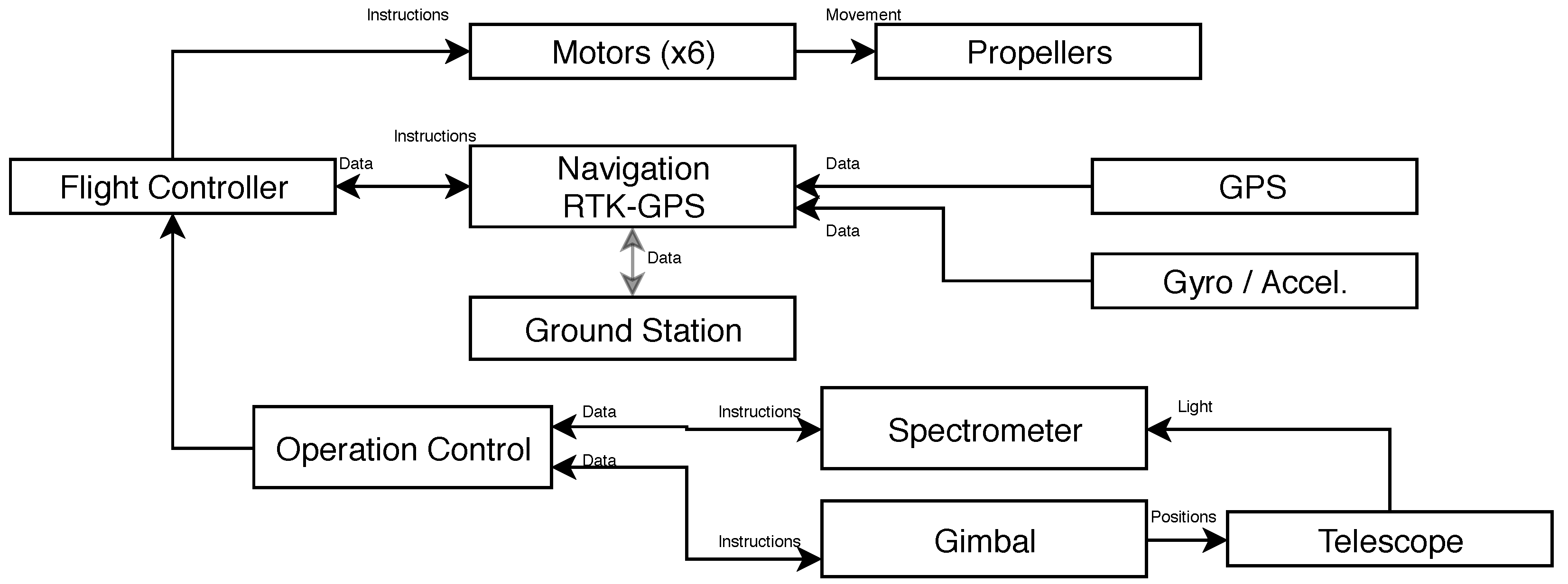
TomoSim is a simulation platform for a drone-mounted atmospheric monitoring system based on DOAS. Although the physical device has not yet been assembled, the team has already compiled a final (or very close) design, which is schematically represented in Figure 2. The reasoning behind the custom design was to increase the maximum payload and allow longer flight times. The team chose to use a DJI S900 frame (hexacopter), manufactured by DJI in China, with custom-made 368 mm carbon fibre arms, longer and lighter than the original. The increased empty space allows the replacement of the default propellers by 17 carbon fibre units, coupled to 6 E1200 motors. This propeller-motor configuration is not only significantly more powerful than the default assembly, but also more efficient. According to the manufacturer [23], this configuration is able to lift and work with payloads exceeding 8 kg, which is much more than we need for data acquisition platform, comprised of the gimbal, a Celera SSIN-06 [24] unit with a maximum pointing error of 2 arcseconds; the telescope, an Omegon MightyMak [25]; and an Avantes Mini spectrometer with 2048 spectral channels [26].
A Pixhawk flight controller is used to handle and manage aerial dynamics, and also to gather every sensor output in the device. The controller comes with integrated gyroscopes, magnetometers and barometers. The only external sensor that needs to be adapted and purchased separately is the navigation (GPS) unit. The Pixhawk supports Real Time Kinematic GPS (RTK-GPS), a combination of inertial sensors and satellite navigational data that can grant the UAV a positioning precision under 20 cm [27,28]. The flight controller is in permanent communication with the operation controller, which is a Raspberry Pi 0 (or similar) single board computer. This computer stores the flight program and directs the flight controller to each necessary position, and also controls data acquisition through a USB connection to the spectrometer. The device’s trajectory will be planned using Arducopter’s Python libraries and their Software In The Loop (SITL) simulation platform.
2.2. Data Acquisition
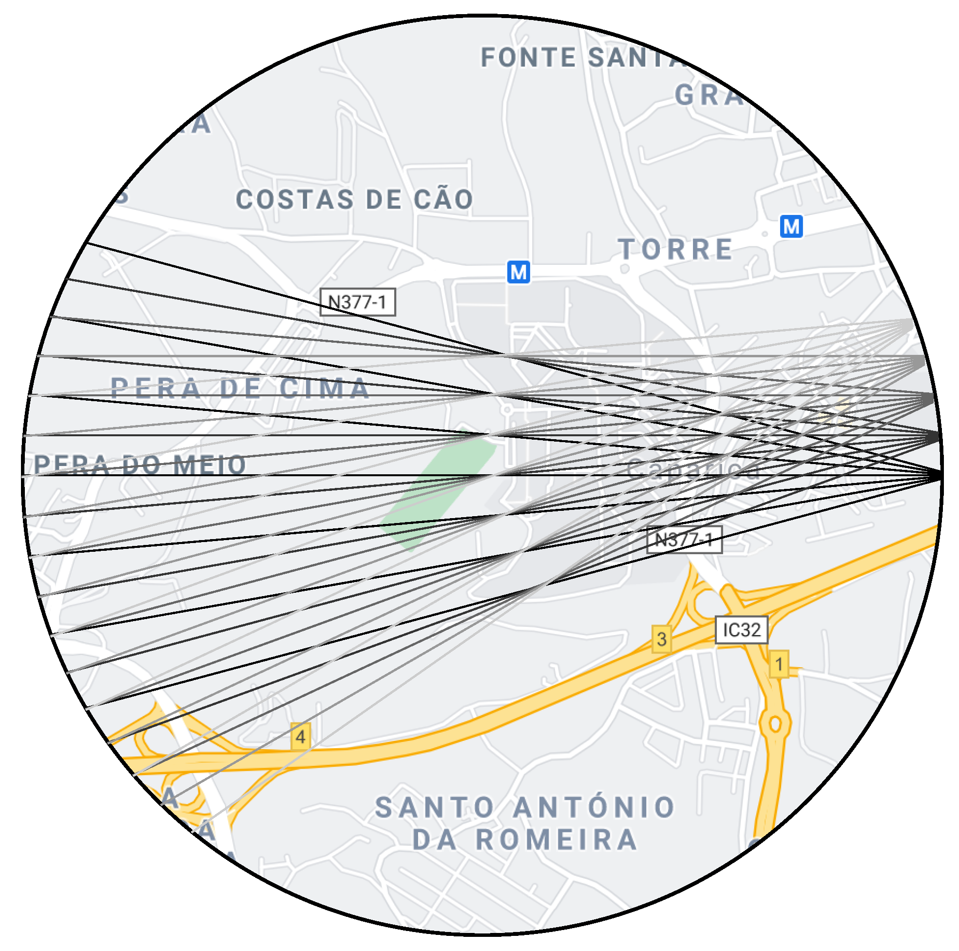
The simulated drone is to describe an unobstructed horizontal circular trajectory with a maximum diameter of 1 km at the intended measurement height, the interior of which is the Region Of Interest (ROI). There are two moments to the data gathering process. Figure 3 attempts to illustrate both.
- First moment While flying in this circle, the device stops in a series of positions at a given fixed angular interval () from each other. The number of stops is defined by and by fan beam information requirements (see Reference [9]) At each one of these stops, the gimbal turns towards the trajectory’s interior and points in a series of angular directions that describe an arc. For procedural simplicity, the angle between these directions is also . At each one of these angles, the device’s operational controller instructs the spectrometer to acquire a given number of spectra, which depends on configuration and conditions. Besides spectral data, the system algebraically calculates and stores the point in which the light will exit the ROI (see Appendix A).
- Second moment The device positions itself in each of the points in which light has exited the ROI in the first moment and the gimbal is pointed towards the entrance point, effectively aiming in the opposite direction to which a spectral measurement took place in the 1st moment. Light that comes from the sun is scattered somewhere in the atmosphere and enters the ROI (at a given angle) in point A. It then traverses the distance AB and leaves the ROI in point B. At these distances and with this kind of geometry, light scattering can be considered negligible [22,29,30] and therefore light extinction will primarily be due to absorption by components between A and B [5]. It should then be possible to apply Lambert-Beer’s law to extract trace gases concentrations in the ROI, by considering light at point A as the source intensity ( in Equation (1)) and light at B the final intensity (I in Equation (1)). When the 2nd moment is complete, the system has a set of fan beam distributed spectra, which can be equated to projections in a tomography problem.
2.3. Phantoms
In medicine, a phantom is a model that emulates certain properties of human or animal tissue. Researchers use these models to evaluate therapeutic or diagnostic methods. In the imaging field, phantoms are known matrices with a given size that were designed to mimic the types of bodies that are to be reconstructed with the technique or algorithm being tested. Most phantoms described in the literature were constructed specifically for medical imaging, since this is clearly the most prominent application field for tomographic methods. Computed Tomography phantoms, for instance, intend to mimic the X-ray absorption of the human body, or of part of the human body. Since the distribution of gases in the atmosphere is entirely different from biological tissue’s, these phantoms are not adequate for TomoSim. This implied the design of a new phantom, based on the idea that a two-dimensional (in this case) Gaussian peak is more appropriate to describe the smoother nature of the distribution of a gas than a series of sharply defined ellipses [31]. The new phantom, designed with TomoPhantom [32], is comprised of 5 bivariate Gaussian profiles, depicting a static gas mixture, and an ellipse near one corner of the image, which serves as a reference point. This new spectral phantom can be seen in Figure 4, and a descriptive summary is provided in Table 1.
During simulation, a phantom is totally contained within the ROI. A gaussian filter (kernel size 5, auto standard deviation) is applied to the phantom image to simulate noise. The phantom shares the same grid as the discretised ROI and each pixel has a value comprehended between 0 and 255. This value is linearly correlated with the number of molecules of the target trace gases in the ROI. Software configuration allows the definition of the maximum number of molecules per pixel. Default value for NO2, the test case presented in Section 3 is molecules.
2.4. Reconstruction
Any tomographic reconstruction requires the previous and detailed knowledge of the ray geometry of the problem. This implies that the space being reconstructed is discretised, so that it can be addressed through computational routines. In this case, the discretisation consists in overlaying a 100 × 100 pixel grid (10 m square pixels, considering a 1 km diameter circular drone trajectory). By applying Siddon’s algorithm to this geometry, the lengths that each ray traverse in each pixel of the grid are retrieved, assembling the system matrix. The system matrix is a complete description of the problem’s geometric properties, and is therefore characteristic of each experiment, depending on the angular intervals between projections ( in this case) and on the size and number of the pixels in the discretisation grid.
TomoSim then performs a resorting operation on the sinogram, in order to transform the fan beam projections into parallel projections, greatly simplifying image reconstruction. Since the angular interval between the fans and the rays within the fans is the same (), resorting is greatly simplified [9]. After discretisation and the necessary resorting steps are taken, the software reconstructs the images with three different algorithms—MLEM, FBP and SART.
Finally, after the images are calculated, the simulator must convert the pixel values back into molecule numbers. For this, the software runs Siddon algorithm on the reconstructed images for a selected number of angles. Resulting projection values are then compared with the projection values of the original images in order to find a converting parameter that allows the presentation of accurate concentration values.
2.5. Error Estimation
There are three major error sources in TomoSim—geometric errors, spectroscopic errors and reconstruction errors. Geometric errors come from the fact that the device’s positioning has an associated error: the drone is not where it thinks it is, nor does it point to where it thinks it points. TomoSim addresses this kind of error in a Monte Carlo like fashion. Positioning and pointing errors are assumed to be normal. Each time a point is calculated, the software generates a normally distributed 0 mean random number, with a standard deviation equal to the rated error of the positioning system and sums it to the intended point (error calculations illustrated in Appendix A). Given the ratios between the linear distances involved in the trajectory and the positioning errors, geometric errors have a very small contribution towards the end results.
On the spectroscopic level, errors come from the instruments used for capturing the data. TomoSim takes this noise into account by adding Gaussian noise spectra to each measurement, for which the magnitude is configurable via its standard deviation, a method previously followed in Reference [33]. This approach is only valid insofar as the captured spectra are perfectly calibrated regarding spectral shift and squeeze, which is an acceptable assumption for a simulation.
Finally, the software has to deal with the reconstruction errors. In image reconstruction from projections, it is common to use techniques such as Mean Squared Error (MSE) as a metric with which to assess the algorithm’s performance. This simulator was also evaluated in this light, in two different ways. First, the MSE for the whole reconstructed image was calculated. This enables the possibility to look at the reconstruction as a whole and visually tell where it is lacking and where it is better performing. Secondly, a score was calculated according to Equation (12). In this equation, and with reference to this simulator, f is the original image and g is the reconstructed image.
Finally, there is an additional source of error that was not explored in this simulation. It is the temporal error that comes from the difference in time between measurement moments (see Section 2.2), which can introduce a larger error than those considered above. In the real world, this can be easily mitigated by the introduction of a second vehicle, which would only conduct 2nd moment measurements. In the simulation, it was considered that there were no changes in the field of measurement with time.
3. Results
This section presents, analyses and discusses results obtained by the application of the techniques and methods described in the previous two sections, that is, the tomographic reconstruction of the phantoms which were also presented in Section 2.
3.1. Projection Calculations
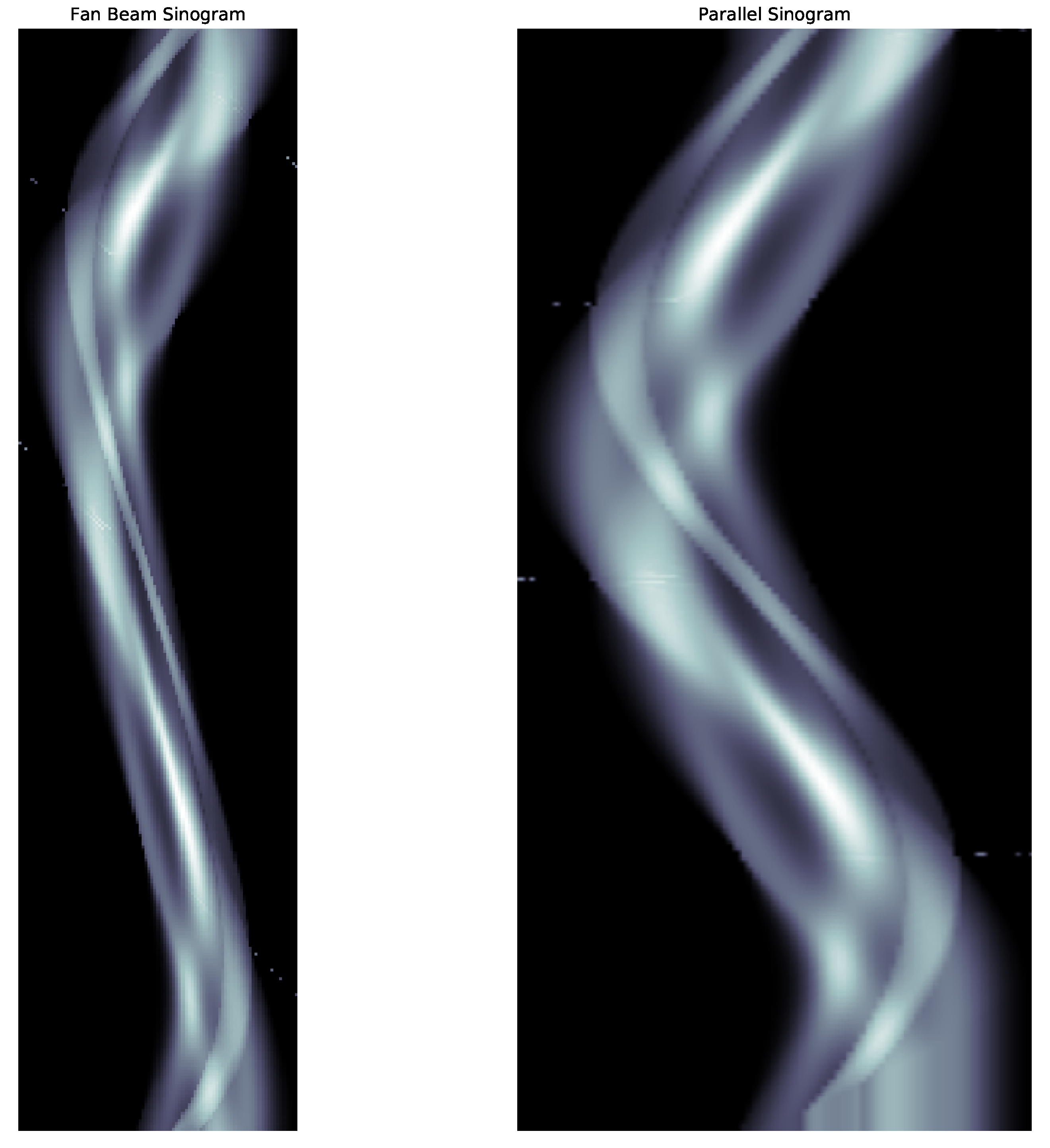
In TomoSim, a projection is the sum of the pixel lengths (the lengths of the rays that traverse each pixel) for each ray and for the grid mentioned in Section 2. Unlike a real life situation, the contents of the ROI are completely known and correspond to the phantoms also described in Section 2 multiplied by a given maximum number of molecules. Siddon’s algorithm is used in this process, and the final results of its application are the sinogram and the system matrix. Figure 5 contains some examples of these matrices, before and after the resorting operation described in Section 2.4.
3.2. Reconstruction Results
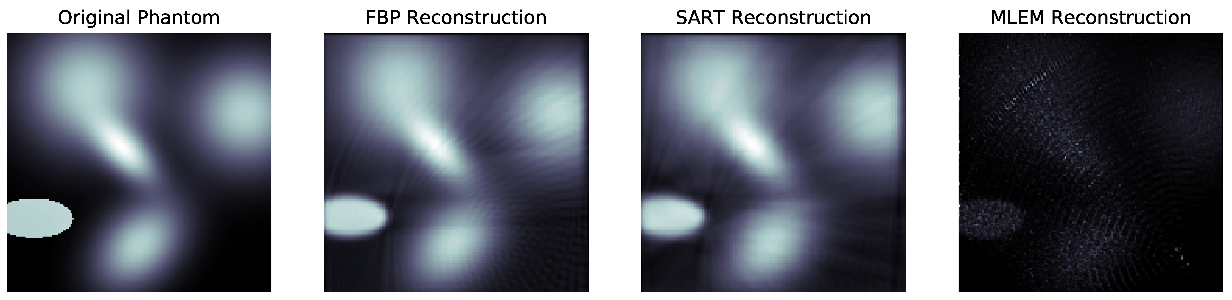
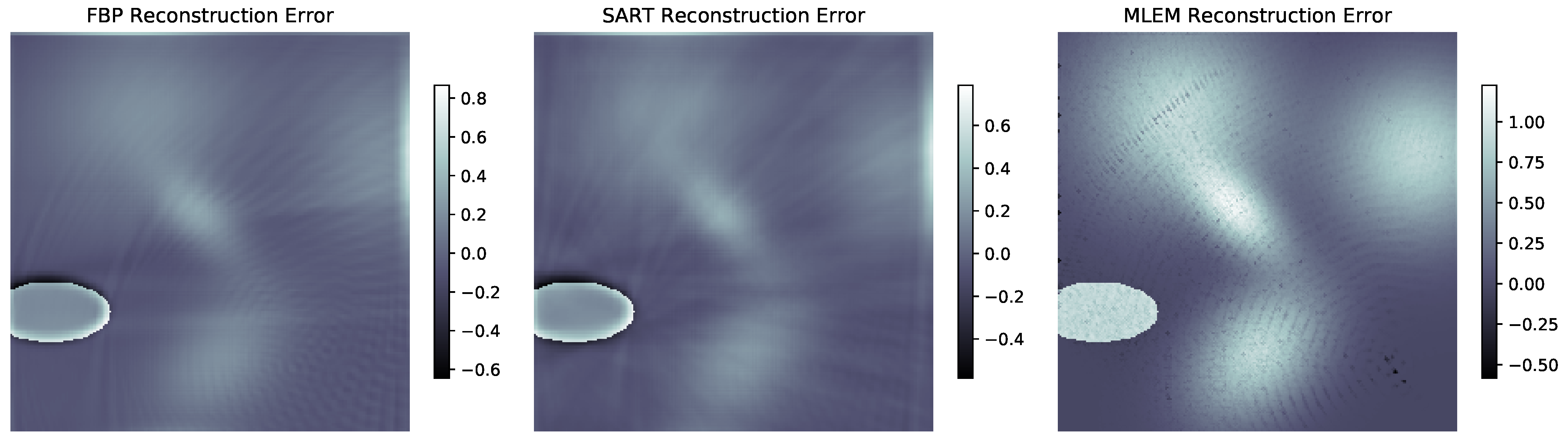
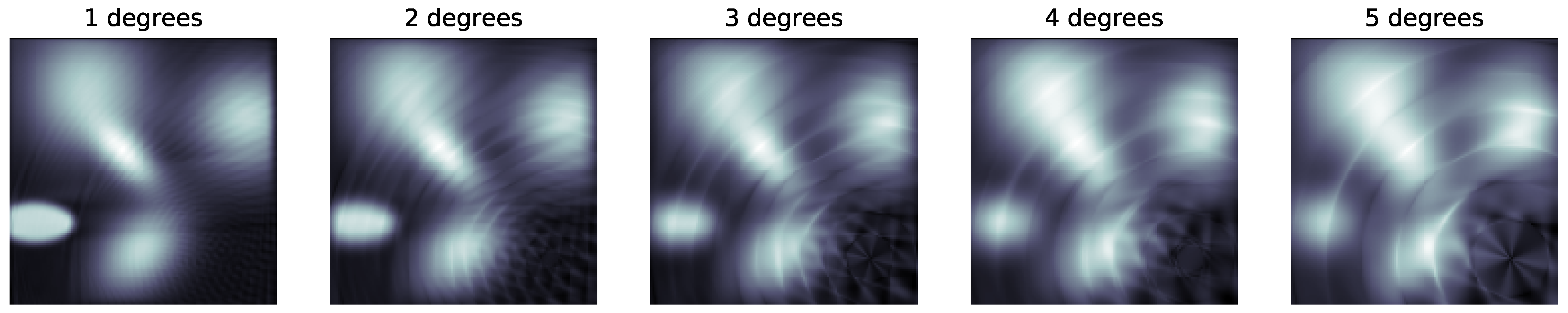
Images corresponding to the trace gas distribution within the ROI were reconstructed using iterative and analytical methods. In Figure 6, one can see the reconstruction results for the three tested methods when applied to the new spectral phantom; Figure 7 shows the graphical representation of the reconstruction errors for the spectral phantom and is accompanied by Table 2; and in Figure 8, a comparison between reconstructions with different values is presented, also for the new spectral phantom.
4. Discussion
The results presented in the previous subsection raise a series of pertinent observations that should be addressed in discussion. The first remark goes to the fact that the number of projections used was adequate to perform the tomographic reconstruction in adequate fashion, as expected. There are already several examples of studies in which a considerably lower number of projections was used, still producing satisfactory results [20]. Moreover, and since the simulation software automatically includes errors in the calculations, this figure also proves that geometric error plays a very limited role in changing the result of the reconstruction. Given the difference in size between the drone’s trajectory and the geometric error, this was also a predicted result.
Even with the relatively low number of projections produced by the drone’s trajectory and measurement strategy, all reconstruction algorithms were able to produce a reconstructed image that resembled the phantom that generated it. , the angular interval between projections, revealed itself to be crucial. This was expected as the number of captured projections is obtained by dividing 360 by . This is, also as expected, confirmed by the upward trend of the error when increasing the value of the angular projection interval, as can be seen numerically in Table 2 and qualitatively in Figure 8. With respect to the algorithms used, the custom-made MLEM routine produces clearly outlier results, which are not on par with the other two reconstruction methods used. This is plain to see both in Figure 6 and in Table 2, in which this algorithm’s NRMSE is almost four times the second best result (FBP) for the smallest projection interval. This difference could to some extent be expected. SART and FBP algorithms were implemented using some of the most relevant and consistently used Python libraries (SciPy, for instance [2]). Given the amount of attention these libraries get from the scientific programming community, levels of optimisation are extremely high. Although it is nowhere near the other two approaches, the MLEM routine is still useful, as it is the only truly geometry-independent algorithm in this study (SART is also geometry independent, but this particular implementation expects a parallel projection sinogram as an input).
As stated in Section 2.5, three different kinds of error influence the reconstruction results: geometric, spectroscopic and reconstruction errors. The first kind of error is directly included in projection calculations, through the application of a Monte Carlo-like method to the geometry described in Appendix A. The second kind of uncertainty comes from the spectrum acquisition process itself, which is not perfect. If one considers there are no systematic errors present in the results, which is an acceptable premise in a simulation, then these errors can be simulated by the inclusion of Gaussian noise in the spectral measurements. This approach is based on the one used in Reference [33], in which a Gaussian noise spectrum is added to the spectrum of interest in order to simulate how the error behaves with a degraded signal. Finally, reconstruction errors come from the finite precision of the calculations that render the images. These errors were presented in Section 3.
The three methods were also evaluated as to how they perform computationally, by measuring the time it took to produce the images in Figure 6 using a Paperspace P4000 cloud computing instance. In this regard, the fastest method was FBP, which took around 3 s to reconstruct. The second was MLEM, with around 50 s for 1000 iterations, and finally came SART, with 1 min and 50 s for 1 iteration. One relevant observation comes from the fact that MLEM was significantly faster than SART, even taking into account the difference in optimisation, which was not an expected result and may indicate some reconstruction enhancing technique on SART’s side, as the literature seems to indicate that this technique is faster than MLEM [15].
All things considered, the FBP algorithm produces a very good reconstruction, equivalent to SART’s, while being more than 10 times faster, indicating that for this kind of application and with this kind of projection information, it is the best reconstruction algorithm.
5. Conclusions
The initial goal of the TomoSim software project was to develop a simulation platform to create the tomographic reconstruction of the column density distribution for a number of target atmospheric trace gases.
The software program was written using the Python language and some numeric calculation libraries, such as NumPy and SciPy. Using these two libraries had two main effects: on the one hand, it enabled the programmers to easily create and manipulate matrices and vectors (images, for instance), and on the other, they greatly improved the running speed of the code, since their core is written in lower level languages (namely C).
The simulations that the software performs prove that, if the final device is programmed to comply to trajectory and acquisition requirements, reconstruction is perfectly achievable, even with relatively low projection numbers (comparing with medical imaging procedures). This brings another significant conclusion which is that the devised acquisition definitions, which produce a set of fan beam arrays, provide sufficient projection information to run the reconstruction and achieve plausible results.
TomoSim runs three algorithms on the projection data in order to produce the spectral mapping of the target pollutants—FBP (analytical), SART and MLEM (both algebraic). SART offered the best results, at the expense of time. The analytical algorithm produced very nearly the same results, but took a fraction of the time when comparing with either SART of MLEM. The MLEM algorithm cannot be directly compared to the SART algorithm, due to differences in the optimisation levels of both routines, but had nonetheless a reasonable time performance altogether, although producing the poorest reconstruction results.
Regarding future developments, there are three main avenues that should be explored:
- Other phantoms: Presently, TomoSim only includes tomographic reconstruction for two different phantoms. While this is sufficient for simulation, it would be desirable to have some more phantoms, which could mimic other concentration distributions of interest.
- Paradigm shift: This simulation software was developed under the passive DOAS analysis model. Active measurements are much more versatile and accurate, and it would be interesting to develop this same technique using an artificial light source. Of course this would require many adaptations, namely regarding equipment and trajectory (probably even algorithms and interpolations).
- Threedimensional reconstruction: TomoSim was developed to produce the reconstruction of a two dimensional image corresponding to the spatial distribution of an array of target trace gases. It would be much more interesting to have a three dimensional equivalent. As far as simulation goes, this is one of the most immediate developments for this project. On a more tangible level, the additional dimensional would make the problem much more complex, mainly because of trajectory and battery logistics.
Author Contributions
Conceptualization, R.V.d.A., N.M. and P.V.; Investigation, R.V.d.A.; Methodology, R.V.d.A. and P.V.; Project administration, P.V.; Software, R.V.d.A.; Supervision, P.V.; Validation, N.M.; Writing—original draft, R.V.d.A.; Writing—review & editing, N.M. and P.V. All authors have read and agreed to the published version of the manuscript.
Funding
This work was funded by Fundação para a Ciência e Tecnologia, grant number PDE/BDE/114549/2016 and UIDB/00645/2020.
Conflicts of Interest
The authors declare no conflict of interest.
Appendix A. Geometric Calculations
Appendix A.1. Light ROI Exit Point (P2) Determination
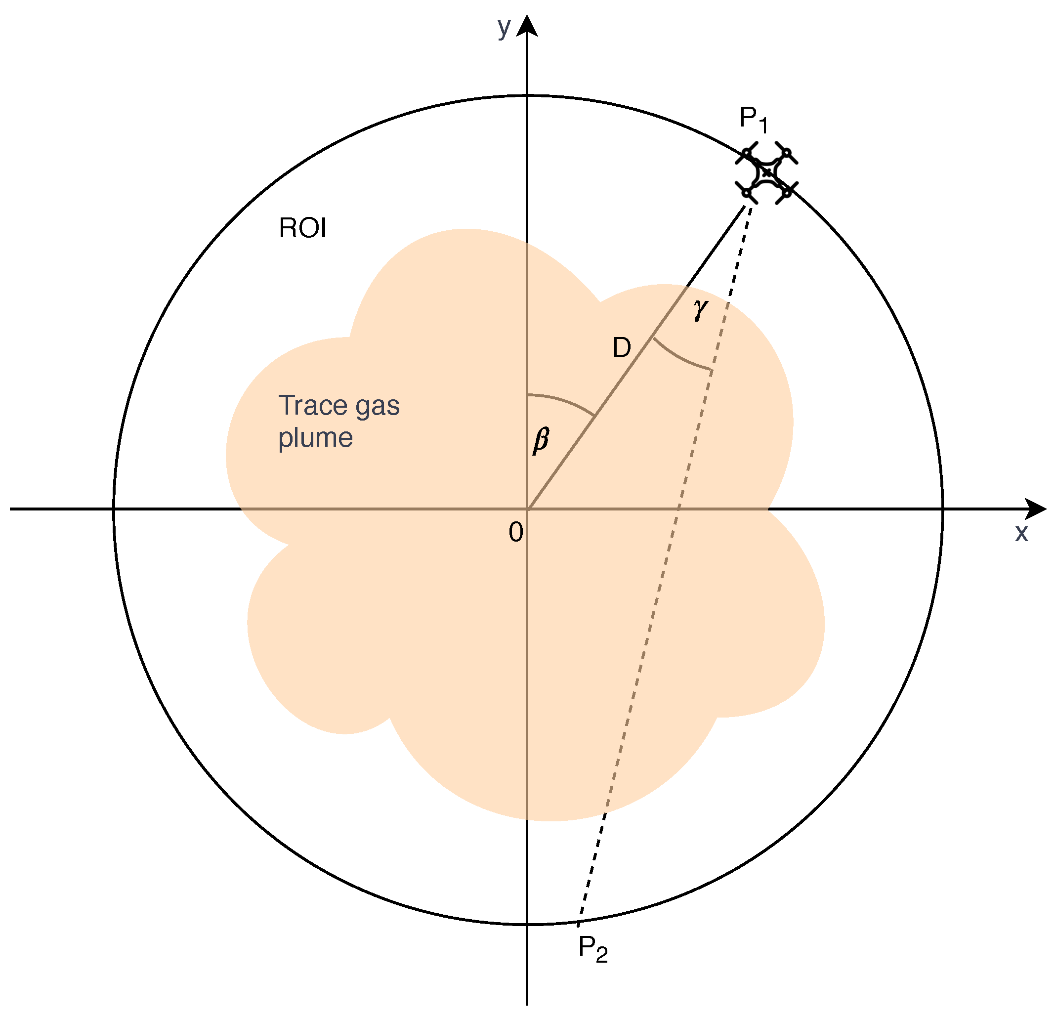
Figure A1 is a schematic snapshot of a point in which the drone is taking a spectrum in one of its stops. Here, the drone’s position, P1, is given by the distance D and the angle , while the gimbal is pointing at a direction at an angular distance of from line 0P1. Point P2, which is not known, is at the intersection between the trajectory’s circumference and line P1P2. Parametrically, any point in this line can be expressed as , with t being a scalar. Moreover, to say a point X is on this circumference is the same as writing . Here, Q is the centre of the trajectory and can therefore be eliminated from the equation. If one is to expand these equations, the situation can be accurately described by Equation (A1).
Unravelling the expressions in Equation (A1), and making use of the algebraic property that says , the expression becomes a two degree equation, as stated in Equation (A2), if one writes as V.
If line P1P2 non-tangentially intersects the circumference, solving Equation (A2) renders two values for t (which correspond to P1 and P2). Selection is made by determining the returned value of t that maximises the euclidean distance between the produced point and P1.
Figure A1.
P2 Calculation.

Appendix A.2. Geometric Error Determination
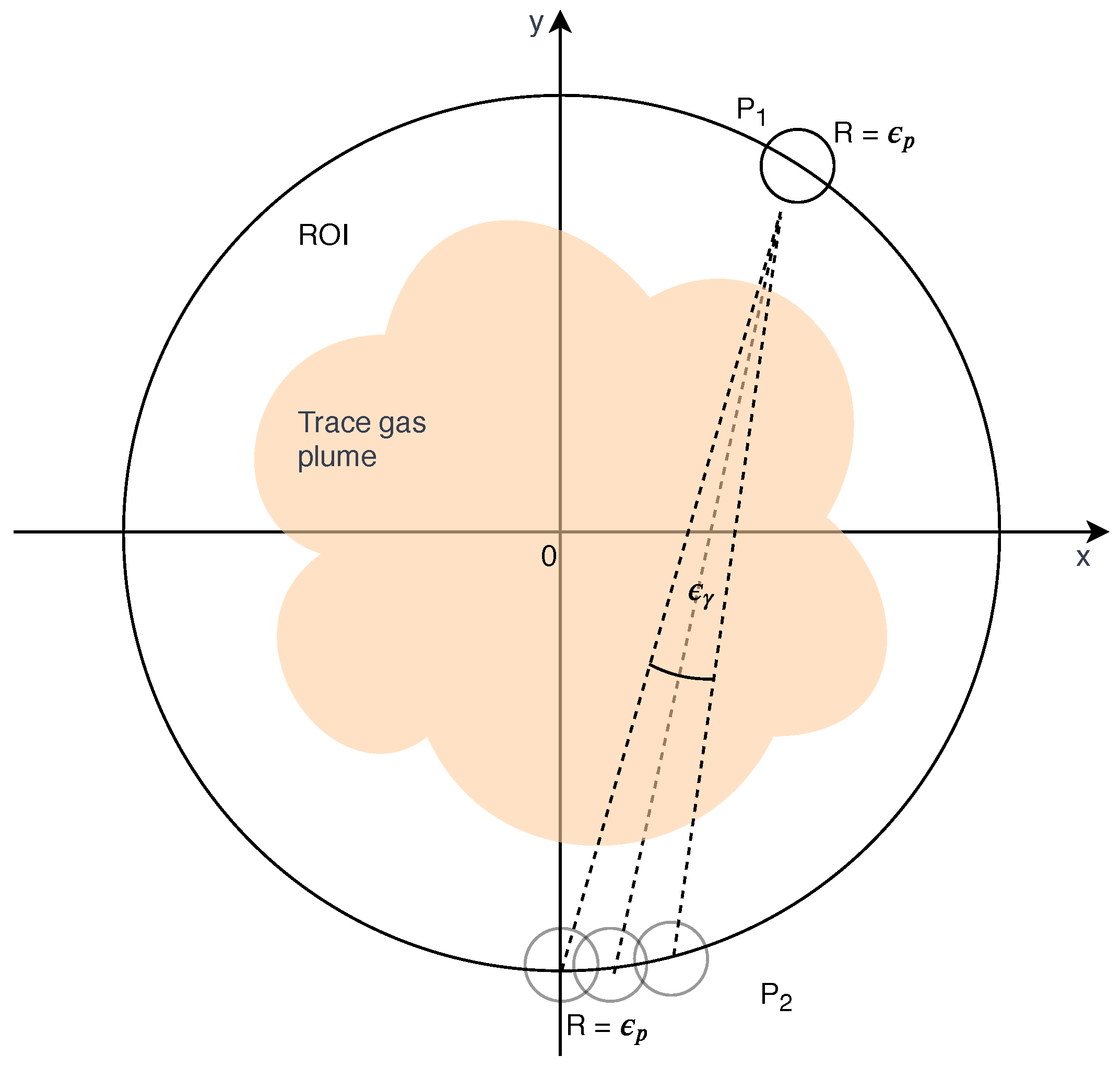
Figure A2 is a graphical representation for the reasoning behind the geometric error estimation. There are two types of error in this image: the ones that come from the RTK-GPS system (positioning error, denoted ) and the ones that come from the gimbal (pointing error, denoted ). TomoSim considers these errors to be normally distributed, and the two values correspond to their standard deviation. To introduce the error into the simulation, the software calculates the theoretical P1 from the and D values (see Figure A1) and then adds a normally distributed random number that respects , retrieving the true P1. This new point is used to draw the theoretical line P1P2 and the pointing error is added using the same process as in P1. Given the very low gimbal error, the small angles approximation () is used to determine the theoretical value of P2, on the drone’s circular trajectory. Finally, the software adds again the positioning error, in the same manner as it had on P1. As a finishing remark, it is important to note that in Figure A2, all errors are extremely exaggerated as they would not be visible otherwise, due to the huge size difference between them and the trajectory.
Figure A2.
Error estimation graphical representation. Note errors are extremely exaggerated for visualisation purposes.
Figure A2.
Error estimation graphical representation. Note errors are extremely exaggerated for visualisation purposes.

Appendix B. Simulation Data Characterization
As stated in Section 2, the simulation uses a phantom matrix to perform its reconstructions. However, this is not purely the input to the simulator routine. Some transforms, introducing random variation, are run beforehand.
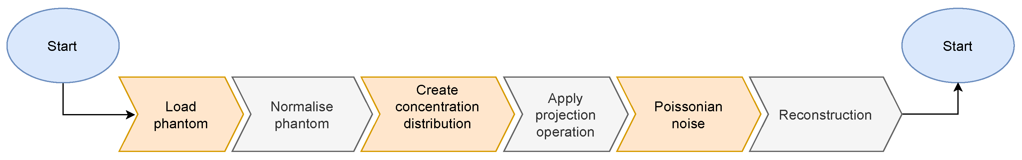
As described in Figure A3, the simulator starts by loading the phantom data. This is a 300 by 300 pixels image, which is created by running the TomoPhantom [32] software. This matrix, which is parametrically stored, is always the same. The data it contains are 64 bit floating point numbers, ranging from 0 to 1 (0 is black; 1 is white). This image is then normalised to range between 0 and 255, and its data type is changed to unsigned 8 bit integers.
The extremes of concentration values are randomly taken from a uniform distribution between and , rendering min_val and max_val. These two values will be used as concentration limits for the phantom matrix, with min_val representing the baseline (0 in the phantom matrix) and max_val representing the maximum value in the ROI (255 in the phantom matrix).
The projection operator which geometrically describes the projection system is applied to the phantom matrix, rendering the sinogram. Before reconstruction, the program adds poissonian noise to this matrix.
Figure A3.
The data flowchart of the simulation routine. The phantom is entered to the routine as a fixed matrix, but is transformed so that each time the program runs, the reconstruction is randomly different and more in line with what happens in nature.
Figure A3.
The data flowchart of the simulation routine. The phantom is entered to the routine as a fixed matrix, but is transformed so that each time the program runs, the reconstruction is randomly different and more in line with what happens in nature.

References
- Perez, F.; Granger, B.E. IPython: A System for Interactive Scientific Computing. Comput. Sci. Eng. 2007, 9, 21–29. [Google Scholar] [CrossRef]
- Oliphant, T.E. Python for Scientific Computing. Comput. Sci. Eng. 2007, 9, 10–20. [Google Scholar] [CrossRef] [Green Version]
- APS. August 15, 1758: Death of Pierre Bouguer. Am. Phys. Soc. News 2011, 20, 2. [Google Scholar]
- Struve, W.S. Fundamentals of Molecular Spectroscopy; Wiler-Interscience: Hoboken, NJ, USA, 1989. [Google Scholar]
- Platt, U.; Stutz, J. Differential Optical Absorption Spectroscopy—Principles and Applications; Springer: Berlin/Heidelberg, Germany, 2007. [Google Scholar]
- Merlaud, A. Development and Use of Compact Instruments for Tropospheric Investigations Based on Optical Spectroscopy from Mobile Platforms. Ph.D. Thesis, Faculté des Sciences—Université Catholique de Louvain, Louvain, Belgium, 2013. [Google Scholar]
- Press, W.H.; Teukolsky, S.A.; Vetterling, W.T.; Flannery, B.P. Numerical Recipes: The Art of Scientific Computing, 3rd ed.; Cambridge University Press: Cambridge, UK, 2007. [Google Scholar]
- Gunderman, R. Essential Radiology: Clinical Presentation, Pathophysiology, Imaging, 2nd ed.; Thieme: New York, NY, USA, 2006. [Google Scholar]
- Kak, A.; Slaney, M. Principles of Computerized Tomographic Imaging; Society of Industrial and Applied Mathematics: Philadelphia, PA, USA, 2001. [Google Scholar]
- Bruyant, P.P. Analytic and iterative reconstruction algorithms in SPECT. J. Nucl. Med. Off. Publ. Soc. Nucl. Med. 2002, 43, 1343–1358. [Google Scholar]
- Herman, G.T. Image Reconstruction From Projections. Real-Time Imaging 1995, 1, 3–18. [Google Scholar] [CrossRef]
- Siddon, R.L. Fast calculation of the exact radiological path for a three-dimensional CT array. Med. Phys. 1985, 12, 252–255. [Google Scholar] [CrossRef] [PubMed]
- Gao, H. Fast parallel algorithms for the x-ray transform and its adjoint. Med. Phys. 2012, 39, 7110–7120. [Google Scholar] [CrossRef] [Green Version]
- Herman, G.T. Fundamentals of Computerized Tomography; Advances in Pattern Recognition; Springer: London, UK, 2009. [Google Scholar] [CrossRef]
- Defrise, M.; Kinahan, P.E.; Michel, C.J. Positron Emission Tomography; Springer: London, UK, 2005; pp. 63–91. [Google Scholar]
- Andersen, A. Simultaneous Algebraic Reconstruction Technique (SART): A superior implementation of the ART algorithm. Ultrason. Imaging 1984, 6, 81–94. [Google Scholar] [CrossRef]
- Shepp, L.A.; Vardi, Y. Maximum Likelihood Reconstruction for Emission Tomography. IEEE Trans. Med Imaging 1982, 1, 113–122. [Google Scholar] [CrossRef] [PubMed]
- Byer, R.L.; Shepp, L.A. Two-dimensional remote air-pollution monitoring via tomography. Opt. Lett. 1979, 4, 75. [Google Scholar] [CrossRef] [PubMed] [Green Version]
- Laepple, T.; Knab, V.; Mettendorf, K.U.; Pundt, I. Longpath DOAS tomography on a motorway exhaust gas plume: Numerical studies and application to data from the BAB II campaign. Atmos. Chem. Phys. Discuss. 2004, 4, 2435–2484. [Google Scholar] [CrossRef]
- Pundt, I.; Mettendorf, K.U.; Laepple, T.; Knab, V.; Xie, P.; Lösch, J.; Friedeburg, C.V.; Platt, U.; Wagner, T. Measurements of trace gas distributions using Long-path DOAS-Tomography during the motorway campaign BAB II: Experimental setup and results for NO 2. Atmos. Environ. 2005, 39, 967–975. [Google Scholar] [CrossRef]
- Stutz, J.; Hurlock, S.C.; Colosimo, S.F.; Tsai, C.; Cheung, R.; Festa, J.; Pikelnaya, O.; Alvarez, S.; Flynn, J.H.; Erickson, M.H.; et al. A novel dual-LED based long-path DOAS instrument for the measurement of aromatic hydrocarbons. Atmos. Environ. 2016, 147, 121–132. [Google Scholar] [CrossRef]
- Frins, E.; Bobrowski, N.; Platt, U.; Wagner, T. Tomographic multiaxis-differential optical absorption spectroscopy observations of Sun-illuminated targets: A technique providing well-defined absorption paths in the boundary layer. Appl. Opt. 2006, 45, 6227–6240. [Google Scholar] [CrossRef] [PubMed]
- DJI. DJI E1200 Pro Tuned Propulsion System. 2015. Available online: https://www.dji.com/pt/e1200 (accessed on 28 December 2020).
- Celera. UAV Gimbal. Available online: https://www.celeramotion.com/applications/satcom-uav/uav-gimbal/ (accessed on 28 December 2020).
- Omegon. MightyMak 60 Specifications. Available online: https://www.omegon.eu/telescopes/omegon-maksutov-telescope-mightymak-60/p,46442#tab_bar_1_select (accessed on 28 December 2020).
- Avantes. AvaSpec-Mini: Small and Powerful OEM Spectrometer. Available online: https://www.avantes.com/products/spectrometers/compactline/avantes-spectrometer-mini-2048cl/ (accessed on 28 December 2020).
- Triantafyllou, D.; Aspragathos, N.A. Intelligent Robotics and Applications—Lecture Notes in Computer Science; Springer: Berlin/Heidelberg, Germany, 2011; Volume 7101, pp. 509–519. [Google Scholar] [CrossRef]
- Zimmermann, F.; Eling, C.; Klingbeil, L.; Kuhlmann, H. Precise Positioning of Uavs—Dealing with Challenging Rtk-Gps Measurement Conditions during Automated Uav Flights. ISPRS Ann. Photogramm. Remote Sens. Spat. Inf. Sci. 2017, 4, 95–102. [Google Scholar] [CrossRef] [Green Version]
- Casaballe, N.; Osorio, M.; Di Martino, M.; Frins, E. Comparison Between Regularized Optimization Algorithms for Tomographic Reconstruction of Plume Cross Sections in the Atmosphere. Earth Space Sci. 2017, 4, 723–736. [Google Scholar] [CrossRef] [Green Version]
- Kern, C.; Deutschmann, T.; Vogel, L.; Wöhrbach, M.; Wagner, T.; Platt, U. Radiative transfer corrections for accurate spectroscopic measurements of volcanic gas emissions. Bull. Volcanol. 2010, 72, 233–247. [Google Scholar] [CrossRef]
- Stachniss, C.; Plagemann, C.; Lilienthal, A.J. Learning gas distribution models using sparse Gaussian process mixtures. Auton. Robot. 2009, 26, 187–202. [Google Scholar] [CrossRef] [Green Version]
- Kazantsev, D.; Pickalov, V.; Nagella, S.; Pasca, E.; Withers, P.J. TomoPhantom, a software package to generate 2D–4D analytical phantoms for CT image reconstruction algorithm benchmarks. SoftwareX 2018, 7, 150–155. [Google Scholar] [CrossRef]
- Stutz, J.; Platt, U. Numerical analysis and estimation of the statistical error of differential optical absorption spectroscopy measurements with least-squares methods. Appl. Opt. 1996, 35, 6041. [Google Scholar] [CrossRef] [PubMed] [Green Version]
Figure 1.
Fanbeam and Parallel geometric assemblies for a tomographic experiment (respectively, left to right). Note that the figures are only meant to exemplify how these assemblies are widely different, and therefore do not have scales or any angular data.
Figure 1.
Fanbeam and Parallel geometric assemblies for a tomographic experiment (respectively, left to right). Note that the figures are only meant to exemplify how these assemblies are widely different, and therefore do not have scales or any angular data.


Figure 2.
Drone system schematic representation, with component relations.

Figure 3.
Simplified schematic representation of the first five fans acquired by the drone over the circular trajectory. The drone stops at the vertex of each fan, represented on the right. These points correspond to point A in the explanation of the two measurement moments in Section 2.2. Each line in the drawing represents a ray within a fan, i.e., a direction, in which a projection is taken. The “exit points” of each ray from the ROI correspond to point B, and are represented on the left. In the second measurement moment, the drone moves to each of these points and takes another spectrum in the same direction as the ray itself. Here, both fans and rays are separated by an angular interval of 5 degrees, and there are only 3 rays within each fan, for graphical simplicity. Both values are customisable at runtime. The map, included for example purposes, was retrieved from Google Maps in 2019 ©Google.

Figure 4.
A graphical representation of the new spectral phantom, custom built for the TomoSim application.
Figure 4.
A graphical representation of the new spectral phantom, custom built for the TomoSim application.

Figure 5.
Sinogram examples: the new spectral phantom projection data at a projection interval of 1 degree. On the left, the projection data before resorting; on the right, the parallel projection data obtained after resorting the fan-beam line integrals.
Figure 5.
Sinogram examples: the new spectral phantom projection data at a projection interval of 1 degree. On the left, the projection data before resorting; on the right, the parallel projection data obtained after resorting the fan-beam line integrals.

Figure 6.
Tomographic reconstruction results, projection interval of 1 degree. From left to right: original phantom, Filtered BackProjection algorithm (FBP) reconstruction, Simultaneous Algebraic Reconstruction Technique (SART) reconstruction, Maximum Likelihood Expectation Maximisation (MLEM) reconstruction

Figure 7.
Tomographic reconstruction errors. Each one of these images was constructed by subtracting the respective reconstruction matrix, displayed in Figure 6, from the original phantom matrix. Error value is normalised to the pixel values, i.e., 32 bit floating point numbers with values between 0 and 1.

Figure 8.
Reconstruction degradation: the projection interval was crucial for reconstruction. Note the image degradation going from a projection interval of 1 degree to 5 degrees (left to right). Images reconstructed using the FBP algorithm.
Figure 8.
Reconstruction degradation: the projection interval was crucial for reconstruction. Note the image degradation going from a projection interval of 1 degree to 5 degrees (left to right). Images reconstructed using the FBP algorithm.


Table 1.
Table summarising the new phantom’s construction details, as a sum of 5 Gaussian profiles and an ellipse designed using TomoPhantom. In this table, C0 is the object’s amplitude, X0 and Y0 are its center coordinates, and a and b are the objects half-widths. The table is constructed using TomoPhantom’s particular syntax and more information can be obtained in Reference [32].
| Type | C0 | X0 | Y0 | a | b | Angle |
|---|---|---|---|---|---|---|
| Gaussian | 1 | −0.1 | −0.1 | 0.25 | 0.5 | −45 |
| Gaussian | 1 | 0.6 | 0 | 0.65 | 0.45 | −45 |
| Gaussian | 1 | −0.6 | −0.4 | 0.8 | 0.8 | 0 |
| Gaussian | 1 | −0.4 | 0.8 | 0.7 | 0.7 | 0 |
| Ellipse | 1 | 0.4 | −0.8 | 0.3 | 0.15 | 0 |
Table 2.
Reconstruction error table for the new spectral phantom at several projection intervals. The MLEM routine used pure fan-beam data while the other two used resorted parallel information. Errors presented were calculated using the Root Mean Square Errors, normalised to the range of the reconstructed image.
| Algorithm | Projection Intervals | ||||
|---|---|---|---|---|---|
| 1 | 2 | 3 | 4 | 5 | |
| FBP | 0.2365 | 0.2408 | 0.2609 | 0.2948 | 0.3465 |
| SART | 0.2225 | 0.2278 | 0.2771 | 0.3537 | 0.3302 |
| MLEM | 0.8705 | 0.9723 | 0.9986 | 0.9744 | 0.9890 |
Publisher’s Note: MDPI stays neutral with regard to jurisdictional claims in published maps and institutional affiliations. |
© 2020 by the authors. Licensee MDPI, Basel, Switzerland. This article is an open access article distributed under the terms and conditions of the Creative Commons Attribution (CC BY) license (http://creativecommons.org/licenses/by/4.0/).
Share and Cite
MDPI and ACS Style
Valente de Almeida, R.; Matela, N.; Vieira, P. TomoSim: A Tomographic Simulator for Differential Optical Absorption Spectroscopy. Drones 2021, 5, 3. https://0-doi-org.brum.beds.ac.uk/10.3390/drones5010003
AMA Style
Valente de Almeida R, Matela N, Vieira P. TomoSim: A Tomographic Simulator for Differential Optical Absorption Spectroscopy. Drones. 2021; 5(1):3. https://0-doi-org.brum.beds.ac.uk/10.3390/drones5010003
Chicago/Turabian StyleValente de Almeida, Rui, Nuno Matela, and Pedro Vieira. 2021. "TomoSim: A Tomographic Simulator for Differential Optical Absorption Spectroscopy" Drones 5, no. 1: 3. https://0-doi-org.brum.beds.ac.uk/10.3390/drones5010003