Article

Modeling Streamflow and Sediment Loads with a Photogrammetrically Derived UAS Digital Terrain Model: Empirical Evaluation from a Fluvial Aggregate Excavation Operation

1
School of Aviation and Transportation Technology, Purdue University, West Lafayette, IN 47907, USA
2
Department of Geography, University of Wisconsin–Eau Claire, Eau Claire, WI 54701, USA
*
Author to whom correspondence should be addressed.
Submission received: 9 February 2021 / Revised: 8 March 2021 / Accepted: 9 March 2021 / Published: 12 March 2021
(This article belongs to the Special Issue Feature Papers of Drones)

Abstract

:
Soil erosion monitoring is a pivotal exercise at macro through micro landscape levels, which directly informs environmental management at diverse spatial and temporal scales. The monitoring of soil erosion can be an arduous task when completed through ground-based surveys and there are uncertainties associated with the use of large-scale medium resolution image-based digital elevation models for estimating erosion rates. LiDAR derived elevation models have proven effective in modeling erosion, but such data proves costly to obtain, process, and analyze. The proliferation of images and other geospatial datasets generated by unmanned aerial systems (UAS) is increasingly able to reveal additional nuances that traditional geospatial datasets were not able to obtain due to the former’s higher spatial resolution. This study evaluated the efficacy of a UAS derived digital terrain model (DTM) to estimate surface flow and sediment loading in a fluvial aggregate excavation operation in Waukesha County, Wisconsin. A nested scale distributed hydrologic flow and sediment loading model was constructed for the UAS point cloud derived DTM. To evaluate the effectiveness of flow and sediment loading generated by the UAS point cloud derived DTM, a LiDAR derived DTM was used for comparison in consonance with several statistical measures of model efficiency. Results demonstrate that the UAS derived DTM can be used in modeling flow and sediment erosion estimation across space in the absence of a LiDAR-based derived DTM.

1. Introduction

Unmanned aerial systems, hereafter referred to as UAS, are now widely recognized in the remote sensing community as a valid geospatial data collection tool. Their utility extends into a wide variety of applications, including but not limited to general mapping, precision agriculture, forestry, wetlands, mining, excavation, and hydrology [1,2,3,4]. While UAS platforms can be equipped with a wide array of sensor types, i.e., meteorological, gas, and particle sensors, the majority of current UAS platforms are equipped with imaging sensors [5,6]. UAS are a useful platform to gather imagery over small to moderately sized areas due to their relatively low cost and for their overall versatility when compared to traditional satellite and manned aircraft remote sensing platforms. Manfreda [7], detailed how traditional manned aircraft and satellites were limited in their ability to gather remotely sensed data based on their altitude constraints and their inability to gather information over certain areas within a given set of time constraints and temporal frequency needs. Furthermore, both satellite and fixed-wing aircraft cannot achieve the centimeter to sub-centimeter spatial resolution that UAS delivers.
The versatility of a UAS platform is best described as being able to fly ‘low and slow’, which means that a UAS platform equipped with a small format camera sensor can fly at a low altitude over a pre-defined area to gather remotely sensed images at resolutions unattainable with traditional platforms, and at a temporal frequency deemed necessary. When UAS imagery is gathered by the platform sensor at a constant altitude, and with enough overlap, the imagery can be processed using structure-from-motion with multi-view stereo (hereafter referred to as SfM) methods to generate a three-dimensional point cloud model [8,9,10]. This point cloud can then be used to generate a digital surface or terrain model (DSM/DTM). A DSM contains all above ground surface features, such as vegetation and buildings, while a DTM only contains the bare ground.
Software companies, such as Pix4D, Agisoft, and Socet Set, have revolutionized the field of photogrammetry by transforming the laborious and time-consuming conventional photogrammetric method into more efficient and optimized workflows such as the scale invariant feature transform [11] and its associated SfM algorithm [12,13,14] including the BAE Systems Socet Set [15]. This new development is timely and welcome in the processing of UAS imagery and extraction of derivatives and is slowly being adopted into the mainstream of many different fields that rely on geospatial data. While the increased use of UAS data is indeed a boon to the geospatial community, the ease of creating SfM derived data products such as a point cloud, DSM, DTM, and orthomosaic means that both the limitations and potential of such data need to be realized.
Despite airborne and terrestrial LiDAR’s accuracy in generating surface and terrain models for use in diverse applications, it is expensive to collect and process, and therefore has limits to its widespread use [7,16,17]. Furthermore, because of the altitude of the platform used, airborne Lidar data is often not available at the 1−2 cm spatial resolution that one can obtain using UAS derived SfM methods [9,18]. While progress has been made toward equipping UAS platforms with LiDAR sensors, the technology remains both cost prohibitive and unreachable for most researchers and UAS users [7,17]. Scientific investigations in the emerging frontier of UAS SfM approaches are needed to better understand the potentially concealed functionalities of photogrammetrically derived UAS data, which might be beneficial in certain research and market niches.
Extraction and excavation-based activities associated with vegetation removal, such as open pit mines, construction sites, barren farm-fields, and post-hazard events (e.g., slope failure) are well-suited for UAS derived DSM and/or DTM analysis [19,20,21]. The lack of vegetation cover associated with surface disturbance on excavated surfaces makes them ideal for modeling both drainage and erosion potential. In an applied sense, the erosion associated with surface drainage at sites devoid of vegetation cover can impact day to day operations at the site. Excessive erosion at construction and mining sites also can mean being subjected to fines and citations from regulatory bodies. Most mining and construction operations are aware of erosion modeling techniques available with LiDAR data, but understand the financial and temporal limitations in place to be able to use such datasets and are seeking means to model surface drainage with technology that is more attainable, such as UAS derived DTM from SfM models.
While LiDAR derived terrain models in hydrologic applications have their place as an essential data source [18], traditional photogrammetrically derived products like digital elevation models (DEMs) are still an important source of topographic information that informs hydrologic applications [22,23]. Historically, such DEM products have been retrieved from medium resolution optical and microwave images [7,24,25]. Quite recently, photogrammetrically derived DSM and DTM from high resolution UAS imagery has been emerging in the hydrologic literature [18,26,27,28]. Photogrammetrically derived UAS data has been used to model surface flow within and outside urban areas [17,29,30], spatial and temporal variability of riverbed hydraulic conductivity [31], channel morphology [32], streambank topography [33], streambank erosion [27], and gully erosion in agricultural and urban watersheds [34,35]. Stocker [34] demonstrated that the photogrammetrically derived data from UAS can measure gully erosion in farmland in a way that LiDAR technology could not due to the increased spatial and temporal resolution that UAS models provide. Gudino-Elizondo et al. [35] reported that UAS derived DSM was effective in estimating gully erosion rates in an urban catchment. While the use of UAS derived dataset to estimate specific types of erosion rates in different catchment characteristics is welcome, we currently know very little on the use and effectiveness of this relatively new dataset to estimate runoff and erosion rates on diverse land cover types [35]. Moreover, an investigation of this phenomenon within the lens of a nested scale distributed hydrologic modeling framework has great potential to unlock the efficacy of UAS derived DTM for the monitoring of runoff and erosion rates across space.
Nested-scale hydrologic modeling framework has proven effective in predicting stream flow and water pollutants when model input data are not available at the same scale [36,37,38]. Didszun and Uhlenbrook [38] applied a nested-scale approach to investigate hydrologic responses at scales < 1 km2 and ≥ 40 km2; they reported slight variation in hydrologic responses at the smallest scale attributed to varying topography. Van der Velde [36] concluded that hydrologic models configured within a nested-scale framework improves prediction of stream discharge and nitrate loads. In a related vein, Zeiger and Hubbart [37] echoed the efficacy of a nested-scale experimental hydrologic modeling design to predict suspended sediment loads. The overarching objective of this study is to assess the potential of a UAS photogrammetrically derived DTM for modeling surface runoff and sediment loading in an open pit fluvial aggregate mining operation experiencing high amounts of erosion. Specifically, this study addresses the following objectives: (1) to develop a downscaling calibration and validation framework for a large-scale hydrologic water quality model and extend to a smaller UAS dataset areal extent; (2) to evaluate the suitability of UAS derived DTM for surface runoff and erosion modeling within an open pit fluvial aggregate mining operation.

2. Materials and Methods
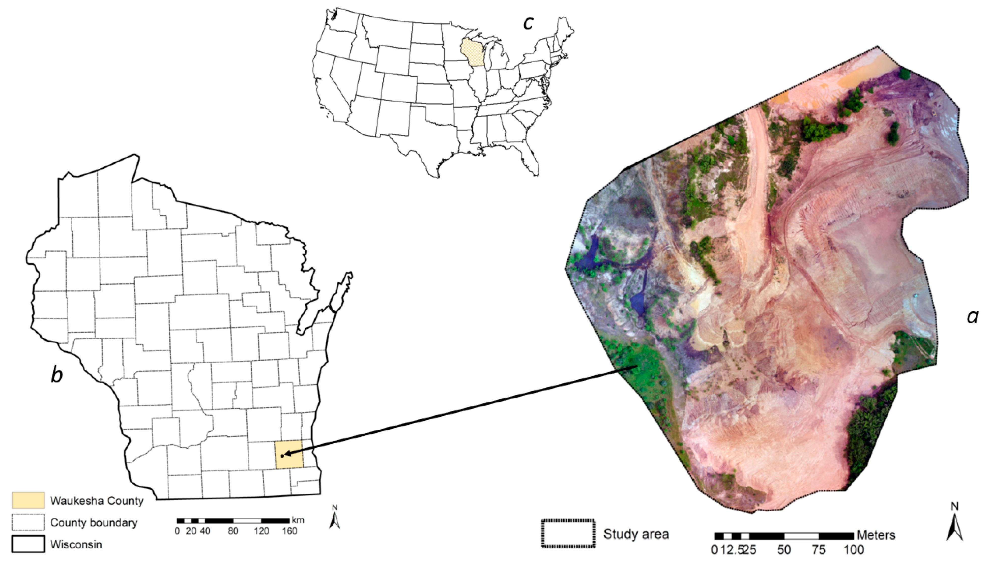
2.1. Study Area

This study was conducted in an open pit fluvial aggregate excavation operation in Waukesha county, near the village of Delafield, Wisconsin, USA. (Figure 1). The operation uses extracted aggregate materials from the open pit for its activities in paving and construction. The data acquisition area covers 10 ha with elevation values ranging between 314 m and 287 m above mean sea level. Due to the erosion issues that the site was experiencing, a request was made to have the area flown with a UAS to potentially identify areas where significant erosion was occurring. The steep slopes and loosely consolidated material made a ground-based survey both impractical and dangerous (Figure 2). The study area is sparsely vegetated (<15%) due to excavation and extraction activities at the site. Average annual precipitation at the site is 87.9 mm. The nearest climatic records from Waukesha, WI show average temperatures in January range from –11.8 to –2.3 °C. Average July temperatures fall within the 27.7 to 15.4 °C range. Soils in the study area are designated as an open gravel pit soil unit and classified as Psammic Fluvent [39].

2.2. UAS Data Collection and Processing

All data was gathered in June 2015 by MenetAero LLC, a UAS service provider who specializes in UAS data acquisition. The Platform used to collect imagery was a DJI Matrice 600 Pro with D-RTK, allowing for reliable flight paths and altitude consistency during flight. Image collection was facilitated by a gimbal based Zenmuse X5 RGB camera equipped with a 15 mm lens (Table 1).
Flight altitude at image capture was 80 m with 80% frontal and lateral overlap. The images were saved onto a 32 GB Generation V SanDisk SD card in Jpeg format. Image geolocation was stored to the image exif file using the WGS 84 geographic coordinate system. This coordinate system is what most UAS platforms utilize to record data related to their GPS log and is the default setting for the DJI platform. It should be noted here that the Matrice 600 Platform, although equipped with D-RTK GPS, did not communicate with the Pix4D Capture application to geolocate the imagery with RTK precision. Spatial accuracy was achieved by the placement and survey of ground control markers prior to the flight. A Trimble R2 GNSS integrated system was used to acquire coordinate locations at six ground control points (GCPs) distributed accordingly across the flight area. To ensure survey quality, redundant check shots were also recorded at each GCP with a variance tolerance of 0.01 m horizontally and 0.02 m vertically. GCPs were recorded using the projected Universal Transverse Mercator coordinate system with a WGS 84 datum. This was chosen to match the desired processed data output projection and coordinate system for further use in a Geographic Information System with other forms of geospatial data.
Pix4D Structure from Motion Multi-View Stereo (SfM MVS) software (version 3.1.23) was used to generate a point cloud, digital surface model, orthomosaic image, and subsequent derivative data products that allowed for further analysis within LP360, ESRI ArcMap Desktop (version 10.7) software, and image processing utilities. Calibration, validation, subsequent processing, and error reporting details associated with SfM model creation utilized in this study are summarized in Table 2 and adhere as best as possible to guidelines put for by James [40]. Following the initial processing phase, where the geolocated images are used to generate a low-density point cloud, the dataset was adjusted for both horizontal and vertical accuracy using the GCP markers. The dataset was then reoptimized and used to generate a high-density point cloud (las format) with 0.058 m RMS error.
Utilizing a hybrid approach, the UAS photogrammetrically derived point cloud was classified into ground and above ground points with the aid of LP360 software (GeoCue Group, Madison, AL, USA). The small fraction of above ground points was a result of shrubs and trees in dispersed throughout study area (Figure 1a and Figure 2a). In the first stage of point cloud classification, we employed the adaptive triangulated irregular network (TIN) ground filter to separate ground points from non-ground points [41,42]. The adaptive TIN-based ground filter generates tiles over the point cloud dataset and identifies the lowest point in each tile as a potential candidate ground point [41]. Next a triangulated irregular network (TIN) is generated from the earmarked lowest points. The algorithm then utilizes thresholds that encapsulates elevation difference and angle closest to a TIN face to iteratively remove non-ground points. Detailed description of the adaptive TIN-based ground filter can be found in Axelsson [41]. In stage two, a two-dimensional profile window that is equipped with vertical manual classification tools was utilized to improve on stage one automated classification. Following the successful classification of ground points, a 3.6 cm DTM was derived by interpolating ground points using a triangulation algorithm. The output spatial resolution of the DTM was set at 3.6 cm to be consistent with the nominal point spacing (NPS) of the classified ground points. A 14.3 cm LiDAR DTM was derived from an already classified LiDAR ground points for Waukesha County collected late spring 2015 [43]. The LiDAR derived DTM spatial resolution was determined by the NPS of LiDAR ground points (~7 points per m2). We used triangulation interpolation method to generate a LiDAR derived DTM to be consistent with that of the UAS derived DTM mentioned above. The final processing of the UAS and LiDAR derived DTMs was the generation of a hillshade for visualization purposes.
In hydrologic modeling, land use/land cover (LULC) are needed to establish parameters related to erosion potential. LULC data was derived from the orthomosaic image of the study area collected during the UAS flight mission. We employed a two-stage hybrid classification framework to generate land cover information for the study area. Object-based image analysis (OBIA) followed by the implementation of a random forest classifier was utilized in stage one image processing [44,45]. The determination of spectral and spatial segmentation parameters was informed by local variance of heterogeneity; following this, image objects were generated by a multiresolution segmentation algorithm [46,47]. Equation (1) illustrates a simplified example of the major segmentation parameters employed in OBIA.
F s =   C w r c + ( 1 C w ) r s
and   0 C w 1
where Fs is segmentation function; Cw is weight given to color; rc illustrates color criterion; and rs denotes spatial criterion. The random forest classifier was trained to classify image objects in conjunction with textural and contextual information [47]. In stage two, output of random forest classification was integrated in an expert system ruleset classifier [48] with the use of ancillary data to improve on the result of stage 1 classification. Ancillary data was obtained by creating patches to fix misclassification encountered during stage 1. Image classification accuracy was conducted by collecting 300 ground reference points via stratified random sampling from a high-resolution National Agriculture Imagery Program (NAIP) imagery collected at the same temporal scale as the orthomosaic imagery [39,49]. Overall image classification accuracy is 89%. At the end of image processing, five classes were produced: Trees, shrub, marshland, loose sediment, and compacted sediment (Figure 2a).

2.3. Flow and Sediment Model Construction

The Soil and Water Assessment Tool (SWAT) was employed to model flow and sediment loading in the study area. SWAT is a fully distributed model that aids in the evaluation of land management practices on flow and water quality in river basins over time [50,51]. For a SWAT model to be successfully implemented, it requires LULC, soil, elevation, and climate variables. Soil data was obtained from the soil survey geographic (SSURGO) data [52] while climate data was acquired from SWAT database. For a SWAT model to produce results that are close to reality, it must be calibrated and validated. We constructed two SWAT models for the UAS derived DTM and the LiDAR derived DTM, respectively. Due to the unavailability of observed streamflow data within the UAS image acquisition area, a nested downscaling approach was developed and applied in operationalizing model calibration and validation. We reconstructed the hydrologically active area covered by the closest USGS streamflow gauging station (4 km upstream) to the UAS study extent. The larger watershed (199 km2) encapsulated the UAS study area and accounted for the hydrologically active area of the observed streamflow data (Figure 3). An ungauged SWAT model with a warmup period of 15 years (2000−2014) was initially operationalized for this larger calibration study area. Following this, the model was calibrated and validated to obtain the appropriate coefficients for 17 key SWAT parameters (Table 3) that were found to be highly sensitive at this large spatial scale and extendible to the smaller UAS spatial scale.
We employed Sequential Uncertainty Fitting version 2(SUFI-2) program embedded in SWAT-CUP 2012 to calibrate and validate the models [53,54]. SUFI2 fits SWAT output simulated data to observed data and in the process adjust the coefficients of SWAT model parameters during model calibration [55]. In evaluating how well a model is calibrated, SUFI-2 utilizes two major criteria. The P-factor which provides a measure of SUFI-2’s ability to capture uncertainty while the R-factor gauges the quality of model calibration [56]. Equation (2) depicts the R-factor.
R =       1 p i = 1 p ( B s , 97.5 % B s , 2.5 % ) i σ o b s  
where p is the number of parameters fitted, Bs,97.5% and Bs,2.5% represents the upper and lower bounds of the 95PPU (95% prediction uncertainty) for a simulated variable Bs, σobs is the standard deviation of the observed data. Values for R-factor range between 0 and infinity. An R-factor of zero demonstrates a perfect fit between simulated and measured data. Figure 3 illustrates a simplified SWAT model used in calibration at the larger spatial extent.
Due to the paucity of monitoring stations in the watershed, a temporal split sampling was used in the calibration and validation for flow [57]. The model was calibrated for flow between August−2015 and August−2016 while validation was implemented between August−2017 and August−2018. To obtain the appropriate calibrated coefficients for the parameters outlined in Table 3, we executed 10,000 iterations. The best simulation that produced the appropriate coefficients for the parameters was achieved at iteration 9457. Following the successful model calibration and validation for flow at the larger spatial extent, the simulated flow value at the subbasin that mostly coincides with the UAS study area location was used as an observed data to calibrate and validate the UAS DTM and LiDAR derived DTM models for flow, respectively. To evaluate the efficacies of model calibration and validation for (i) the large extent SWAT model, and (ii) the UAS DTM and LiDAR derived DTM models for flow, three additional statistical measures besides that outlined in Equation (2) were employed.
The first additional statistical measure used to evaluate model effectiveness for calibration and validation is the Nash–Sutcliffe (NS) coefficient [58]. Equation (3) illustrates the Nash–Sutcliffe coefficient:
E   =   1   i = 1 n ( O i S i ) 2 i = 1 n ( O i O ¯ ) 2
where E is the Nash–Sutcliffe coefficient of model efficiency, Oi is observed data; Ō is the mean of observed data; Si is simulated value, while n is the total number of observations. Possible values of NS range between –ꝏ and 1.0. A Nash–Sutcliffe statistic of 1.0 suggest a perfect fit between simulated and observed data, NS values between zero and 1 are generally regarded as tolerable levels of model performance, while NS values less than zero illustrates that the mean of observed data is a preferred predictor compared to the simulated values. Another model efficiency criterion that we employed is the index of agreement (d) which is calculated according to the following equation [59]:
d   =   1     i = 1 n ( O i S i ) 2 i = 1 n ( | S i O ¯ | + | O i O ¯ | ) 2   0     d     1
where d is the index of agreement, Oi is observed signal, Ō is the mean of observed signal, Si is simulated value, while n is the number of observations. An index of agreement value of 1 suggest perfect fit between simulated and observed while zero depicts no association. We further employed the root mean square error (RMSE) in evaluating model predictive power [60]. The RMSE statistics quantifies the predicted error (residuals) vis à vis the units of the simulated value into a single measure of model efficiency. The RMSE is calculated according to the following equation:
RMSE   =   i = 1 n   ( O i S i ) 2 n
where Oi and Si represent observed and simulated values of a sample size n. Values for RSME range between 0 and ꝏ, where RMSE of zero suggest perfect fit between observed and simulated information.
Calibration of suspended sediments was not performed due to the unavailability of suspended sediment observed data covering the accepted period of model calibration and validation, outside SWAT warm up period (2000–2014). Notwithstanding, one pivotal sediment related SWAT parameter (PRF) that is tied to flow parameters was calibrated thus providing an indirect calibration for suspended sediment (Table 3).
Figure 4 shows a simplified SWAT model constructed for the UAS spatial extent using a LiDAR derived DTM (Figure 4a) and a photogrammetrically derived point cloud DTM (Figure 4b). In each of the models, the watershed was automatically delineated into 60 sub-basins with very similar characteristics of monitoring points, stream network, and sub-basin sizes and morphology.
Both models were calibrated and validated for flow at the monitoring points marked with red circle in Figure 4a,b. The warmup period including calibration and validation period for the SWAT models was consistent with that assigned to the large spatial extent illustrated in Figure 3.

3. Results and Discussion

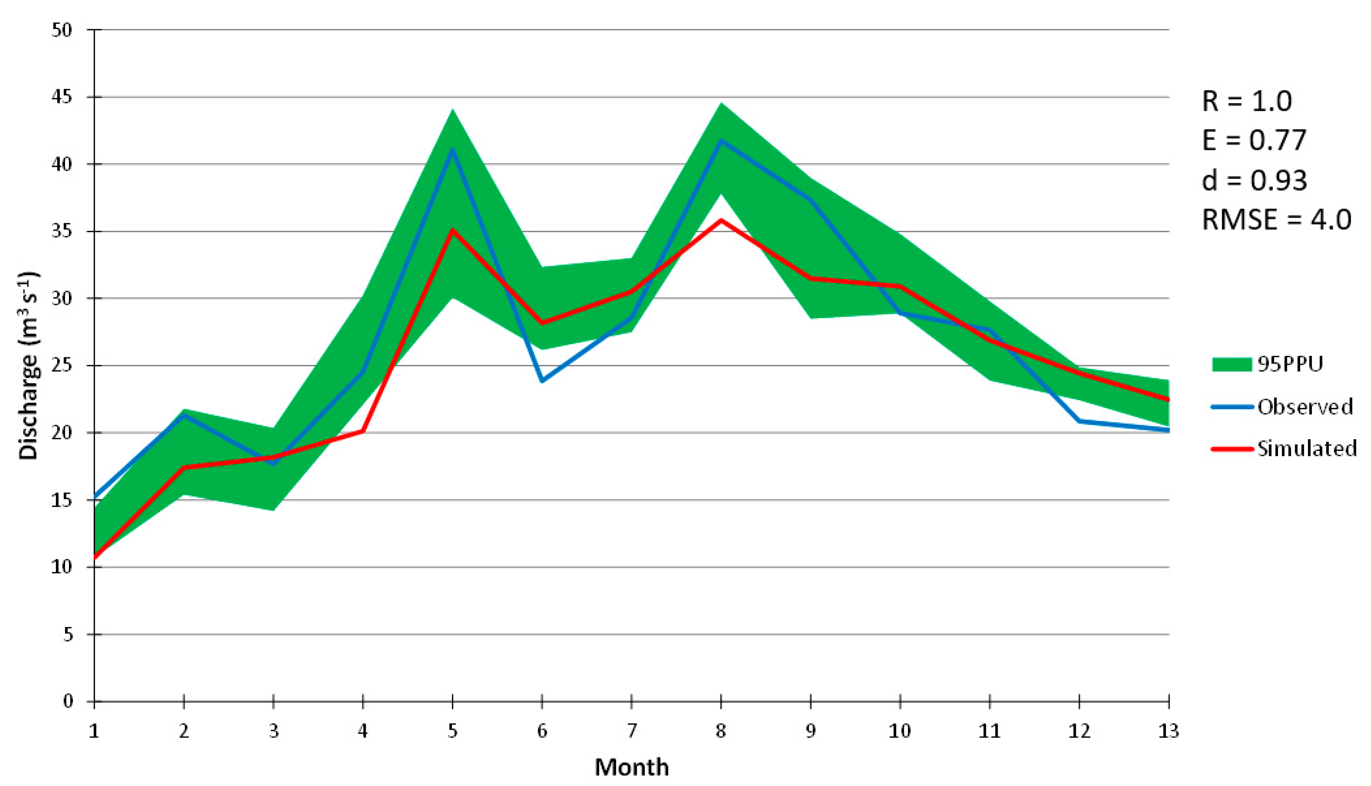
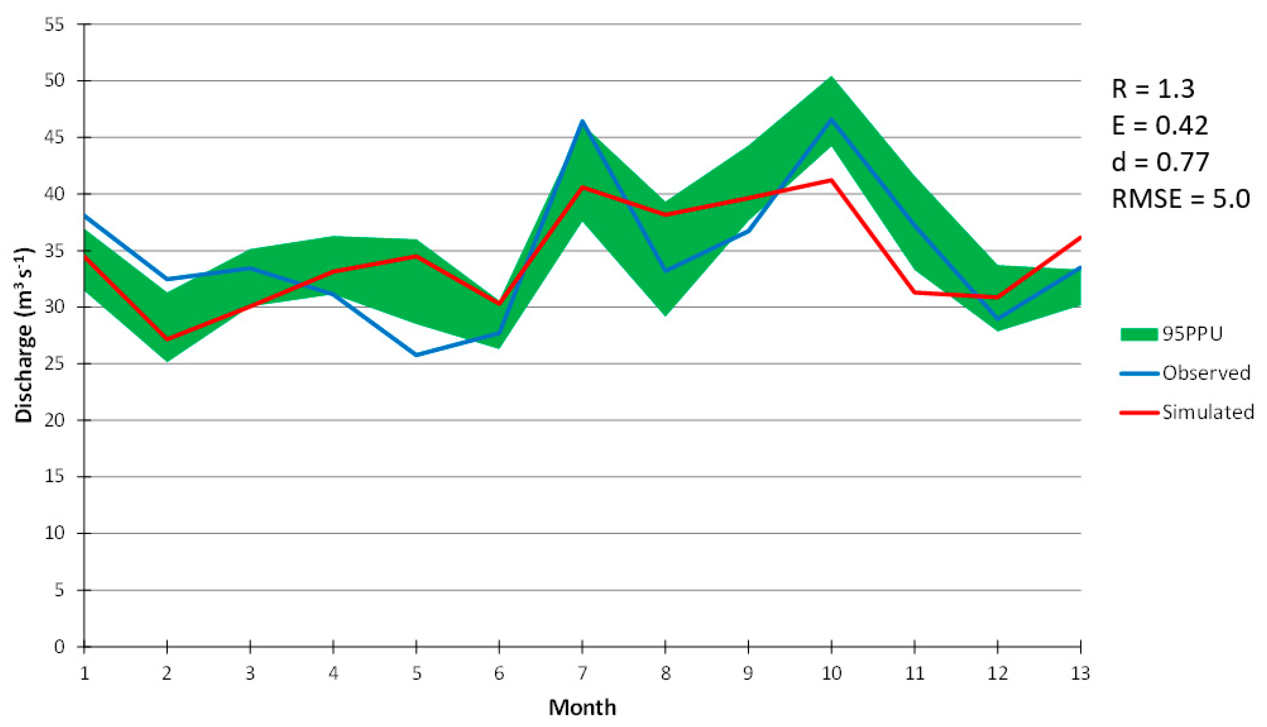
3.1. Model Calibration and Validation at the Larger Spatial Extent

The SWAT model was calibrated for flow between August 2015 through August 2016 at a monthly timestep. In Figure 5, the statistical measures of model efficiency clearly demonstrate that the simulated flow is within acceptable threshold of the USGS measured data. Moreover, all the measures of model efficiency demonstrated that the 17 SWAT parameters outlined in Table 3 did a decent job in fitting the simulated data to the USGS observed streamflow data. The extent of model uncertainty captured by the 95PPU (>76%) further attest to the effectiveness of the model calibration. The R-factor (R), Nash–Sutcliffe (E), and index of agreement (d) shows strong association between simulated and observed data. Despite the relatively low RMSE, the overwhelmingly excellent efficiency of the other criteria suggests that the model calibration is robust.
Note: R is R-factor, E is Nash–Sutcliffe coefficient of simulation efficiency, d is index of agreement, and RMSE is root mean square error.
The SWAT model was validated for flow between August 2017 and August 2018 at a monthly time interval. The model evaluation criteria of R, E, and d (Figure 6) are not that different from those demonstrated for model calibration and suggest a strong validation of the model, though one can conclude the model was slightly better calibrated compared to its validation. Notwithstanding, all the statistical criteria strongly suggest that the model was constructed in a manner that closely matches surface fluvial hydrologic characteristics. Figure 6 also shows that a large fraction (>80%) of model uncertainty was captured by the 95PPU. The widely used model efficiency values generated by Nash–Sutcliffe, index of agreement, and the RMSE are within acceptable levels reported in other studies [61,62,63].
Note: R is R-factor, E is Nash–Sutcliffe coefficient of simulation efficiency, d is index of agreement, and RMSE is root mean square error.

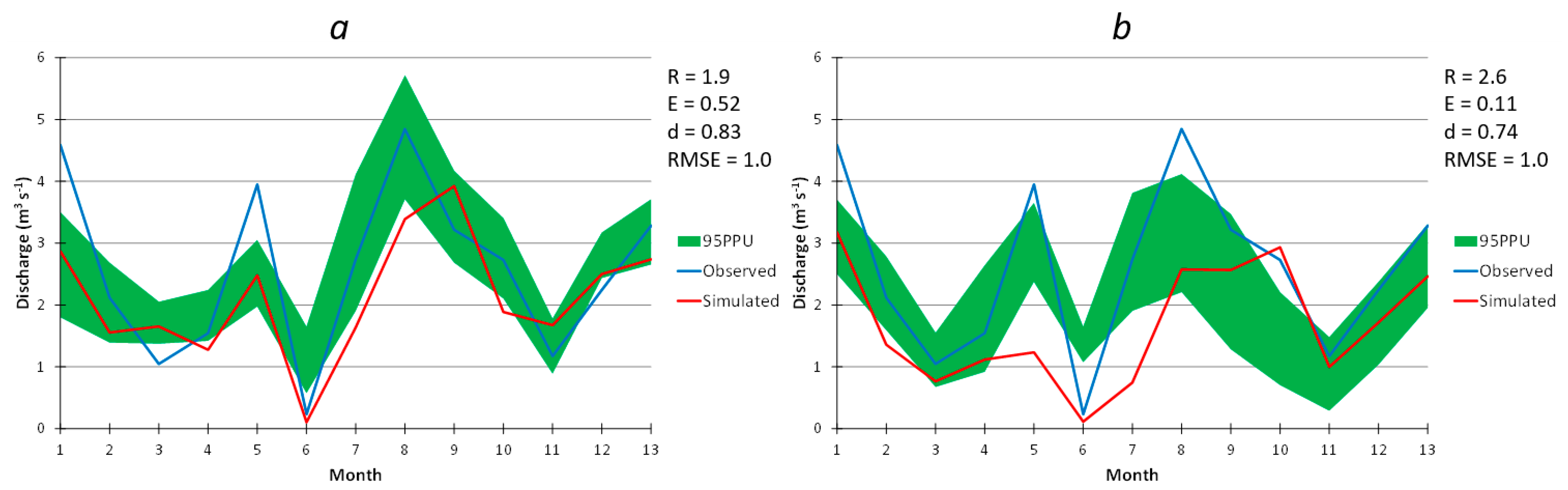
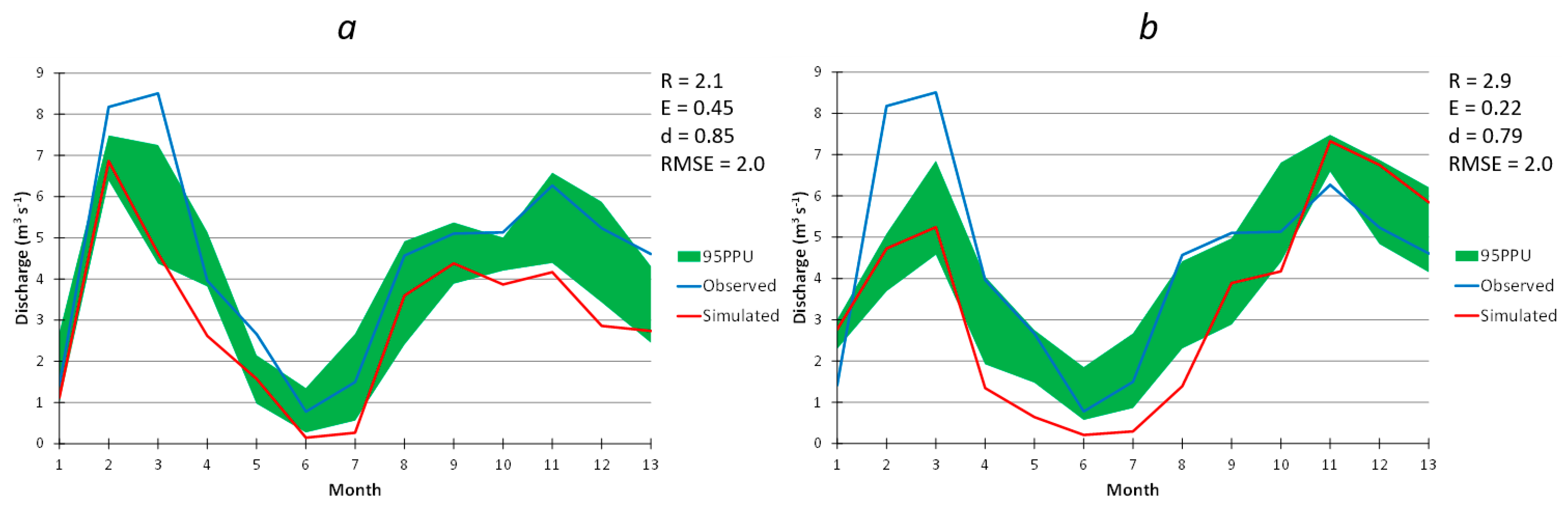
3.2. Model Calibration and Validation at the UAS Spatial Scale

Following the successful calibration of the large spatial extent SWAT model, the fitted parameter coefficients were transferred to the nested UAS spatial scale models. Moreover, the predicted streamflow at the sub-basin closest to the UAS spatial extent watershed was used for calibrating and validating the models. It has been shown that model parameters and their coefficients are regionally transferrable within a watershed if the efficiency value statistics are reproducible at a different sub-basin [64]. Calibration results for the UAS derived DTM and Lidar derived DTM demonstrated that both models fall within an acceptable threshold of model calibration efficiency despite the LiDAR derived DTM having a relatively higher R-factor, Nash–Sutcliffe, and index of agreement (Figure 7). Notwithstanding, both models had identical RMSE which turned out to be higher than that obtained at the larger spatial extent scale of calibration. The models generated by the LiDAR DTM and the UAS DTM, respectively also illustrated that a high fraction (>70%) of model uncertainty was captured during calibration as can be seen by the 95PPU. As a result of the model calibration, it can be subsequently concluded that a photogrammetrically derived DTM from a UAS point cloud is effective in modeling flow. Jeziorska et al., [30] reported that a UAS derived terrain model is more effective in accounting for flow morphology and patterns over a lidar derived DTM in areas not covered by vegetation because of its increased spatial resolution. We attribute the slightly lower values of R, E, and d in the UAS derived terrain model to the uncertainty in interpolated terrain beneath the few areas within the watershed that are covered by trees and shrub and also to the single flow (D-8) algorithm used by SWAT. Studies have shown that a multiple flow algorithm better estimates flow compared to single flow algorithm [65,66]. Figure 8 shows the validation results for the LiDAR derived DTM and UAS derived DTM. Both models are within the acceptable threshold of validation based on their simulation efficiency despite the Lidar based DTM scoring slightly higher values compared to the UAS derived DTM in three of the four model efficiency criteria used (Figure 8).
Validation results for the two models display close similarities when compared to the results generated by calibration. This suggest that a UAS-derived DTM can serve as an alternative dataset to model streamflow in the absence of lidar DTM provided that the study area has minimal to no vegetation cover. When vegetation cover dominates a study area, ground/terrain models generated by UAS-derived point cloud contains higher errors [67,68] and may not be suitable for modeling streamflow. Since surface runoff is mostly controlled by terrain, we recommend that a UAS derived DTM used for estimating flow and eventual sediment erosion be collected over areas with minimum high vegetation cover, such as trees (<10%). Moreover, as demonstrated by Jensen and Mathews [69], the point cloud should be classified into ground points using a robust algorithm such as the adaptive TIN ground filter employed in this study followed by a manual classification of the automated classified ground points to further eliminate above ground features. The resulting DTM generated from the hybrid classified ground points can be used in modeling flow across space in the absence of a LiDAR derived DTM. This refined UAS derived DTM has great potential to extend the applications of UAS data.

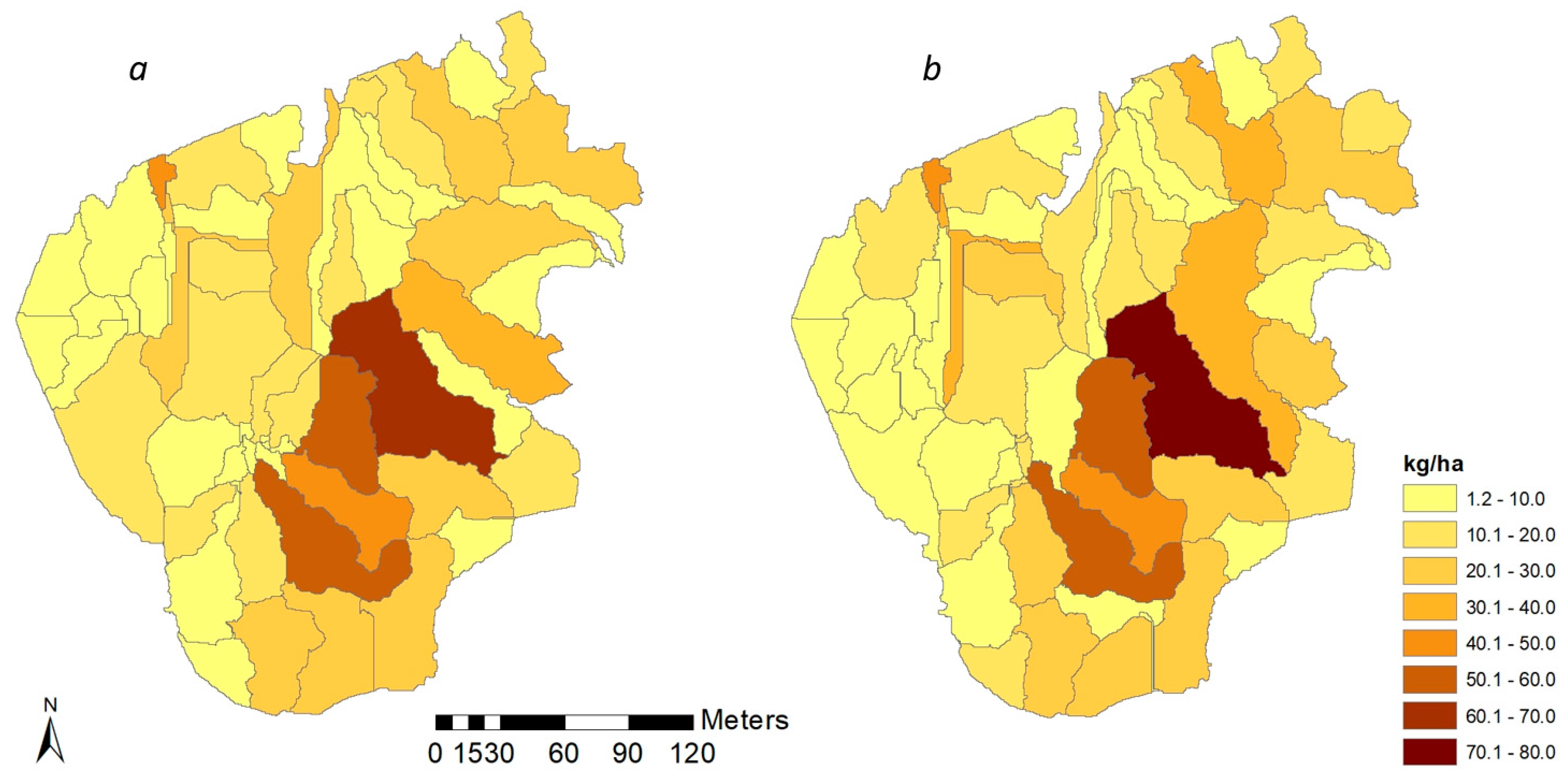
3.3. Assessment of Sediment Erosion at the UAS Spatial Scale

The calibrated and validated SWAT models for the LiDAR point cloud DTM and photogrammetrically derived point cloud DTM were used to model the amount of sediment being eroded and washed from the watershed at the sub-basin level. Figure 9 compares the sediment loads generated by the two models. The photogrammetrically derived point cloud DTM accounted for a slightly higher sediment loading from the watershed compared to that obtained from the LiDAR derived DTM (Figure 9). In sub-basins covered with loose sediment and gentle slopes, the amount of sediment eroded is identical between the LiDAR derived DTM and the UAS-derived point cloud DTM. However, this is not the case in sub-basins that have rugged terrain where the UAS derived DTM generated greater sediment loads compared to the LiDAR derived DTM. We speculate that this difference might be ascribed to the higher spatial resolution of the UAS derived DTM (3.6 cm) compared to the relatively lower spatial resolution of the LiDAR derived DTM (14.3 cm). Digital terrain models derived from UAS point cloud have been shown to be more effective in accounting for streambank erosion [27,33] and measuring gully erosion rates [34] compared to LiDAR -derived DTMs. This effectiveness demonstrates how photogrammetrically derived SfM terrain when used in scenarios with little to no vegetative ground cover, can serve as a low-cost viable alternative to more costly methods that rely on LiDAR data.
Additional research is needed to better compare UAS and LiDAR derived DTMs collected at identical spatial and temporal resolution over non-vegetated terrain to comprehensively evaluate the efficacy of the UAS derived DTM in estimating flow and erosion of sediment. Moreover, the key difference unearthed in this study where both DTMs performed identically in gentle slopes and loose sediments but differently in rugged terrain needs further testing in similar site setting. As the cost of lighter payload LiDAR sensors developed for drone platforms becomes cheaper [70], hydrologic modeling of flow and nonpoint source pollutants which have been historically conducted at moderate to large scales will become more practical at the smaller UAS spatial scale thus providing a more effective tool for monitoring of erosion at mining sites.

4. Conclusions

Unmanned Aerial Systems have been long recognized for their ability to acquire imagery over areas of interest with spatial resolutions that can provide incredible amounts of detail, both temporally and spatially. Coupled with their ability to be quickly deployed over small areas on a frequent basis, UAS have rapidly demonstrated themselves as a valid data collection tool in many geomorphic and geologic applications. While UAS derived data products, such as DSM and DTM have been used in many forms of fluvial research, the integration of UAS derived DTM in a nested scale distributed hydrologic modeling that this study investigated is a unique domain in UAS application. In this research we assessed the feasibility and efficacy of a photogrammetrically derived DTM in modeling sediment erosion across space. The nested scale hydrologic modeling framework successfully downscaled streamflow data from a larger spatial extent and applied to a smaller UAS spatial scale. In this study, we have demonstrated that it is possible to extend the use of UAS derived DTM from river and other narrow transects to the entire image area in modeling erosion potentials. We built on the literature which mostly agrees that the higher spatial resolution obtained from UAS derived products facilitates the modeling of erosion at the transect level. The study also demonstrates that with the tools of model calibration and validation, it is possible to utilize UAS derived DTM to model flow and sediment load estimation in the absence of measured data at the UAS spatial scale. Notwithstanding, we caution that if LiDAR data is available at a higher temporal and spatial frequency, such as the recent lighter payload lidar sensors that can be mounted on UAS platforms, it should be used to monitor flow and sediment loading rather than a photogrammetrically derived DTM especially if the study area is covered with significant vegetation. The nested scale methodology developed and utilized in this study can be extended to similar fluvial aggregate excavation operations. The hydrologic modeling framework serves as an excellent example of how UAS data can serve as a low-cost alternative to LiDAR in terms of decision making and lowering overhead costs in a variety of extraction-based industries. Future research should evaluate the quality and accuracy of models over areas with diverse amounts of vegetation cover and provide a direct comparison of DTM models gathered via LiDAR and UAS imagery, respectively.

Author Contributions

This article was written jointly by J.P.H. and C.O.W. The project was conceptualized and it methodology designed as a joint endeavor between the two authors, where C.O.W. took on a main role of engaging in the GIS modeling while data collection and preliminary analysis was done by J.P.H. Formal analysis of the data was done predominantly by C.O.W. Writing, reviewing, and editing was joint effort between the two co-authors. Both authors have read and agreed to the published version of the manuscript.

Funding

This research was funded by The University of Wisconsin Regent Scholar Award, awarded to J. H. for his work title ‘Lowering Overhead Costs within the Industrial Aggregate and Sand Mining Industry using Unmanned Aerial Systems’.

Institutional Review Board Statement

Not applicable.

Informed Consent Statement

Not applicable.

Data Availability Statement

Not applicable.

Acknowledgments

The authors would like to thank P. M. from Menet Aero for conducting the flights and performing the ground control point survey.

Conflicts of Interest

The authors declare no conflict of interest related to this study. The funders had no role in the design of the study; in the collection, analyses, or interpretation of data; in the writing of the manuscript, or in the decision to publish the results.

References

  1. Huang, S.; Tang, L.; Hupy, J.P.; Wang, Y.; Shao, G. A Commentary Review on the Use of Normalized Difference Vegetation Index (NDVI) in the Era of Popular Remote Sensing. J. For. Res. 2021, 32, 1–6. [Google Scholar] [CrossRef]
  2. Demario, A.; Lopez, P.; Plewka, E.; Wix, R.; Xia, H.; Zamora, E.; Gessler, D.; Yalin, A.P. Water Plume Temperature Measurements by an Unmanned Aerial System (UAS). Sensors 2017, 17, 306. [Google Scholar] [CrossRef] [PubMed] [Green Version]
  3. Bellvert, J.; Zarco-Tejada, P.J.; Girona, J.; Fereres, E. Mapping Crop Water Stress Index in a ‘Pinot-Noir’ Vineyard: Comparing Ground Measurements with Thermal Remote Sensing Imagery from an Unmanned Aerial Vehicle. Precis. Agric. 2014, 15, 361–376. [Google Scholar] [CrossRef]
  4. Lelong, C.C.D.; Burger, P.; Jubelin, G.; Roux, B.; Labbe, S.; Baret, F. Assessment of Unmanned Aerial Vehicles Imagery for Quantitative Monitoring of Wheat Crop in Small Pots. Sensors 2008, 8, 3557–3585. [Google Scholar] [CrossRef] [PubMed]
  5. Singh, K.K.; Frazier, A.E. A Meta-Analysis and Review of Unmanned Aircraft System (UAS) Imagery for Terrestrial Applications. Int. J. Remote. Sens. 2018, 39, 5078–5098. [Google Scholar] [CrossRef]
  6. Tang, L.; Shao, G. Drone Remote Sensing for Forestry Research and Practices. J. For. Res. 2015, 26, 791–797. [Google Scholar] [CrossRef]
  7. Manfreda, S.; McCabe, M.F.; Miller, P.E.; Lucas, R.; Pajuelo Madrigal, V.; Mallinis, G.; Ben-Dor, E.; Helman, D.; Estes, L.; Ciraolo, G.; et al. On the Use of Unmanned Aerial Systems for Environmental Monitoring. Remote. Sens. 2018, 10, 641. [Google Scholar] [CrossRef] [Green Version]
  8. Zhang, H.; Aldana-Jague, E.; Clapuyt, F.; Wilken, F.; Vanacker, V.; Van Oost, K. Evaluating the Potential of Post-processing Kinematic (PPK) Georeferencing for UAV-Based Structure-from-Motion (SfM) Photogrammetry and Surface Change Detection. Earth Surf. Dyn. 2019, 7, 807–827. [Google Scholar] [CrossRef] [Green Version]
  9. Westoby, M.J.; Lim, M.; Hogg, M.; Pound, M.J.; Dunlop, L.; Woodward, J. Cost-Effective Erosion Monitoring of Coastal Cliffs. Coast. Eng. 2018, 138, 152–164. [Google Scholar] [CrossRef]
  10. Clapuyt, F.; Vanacker, V.; Van Oost, K. Reproducibility of UAV-Based Earth Topography Based on Structure-from-Motion Algorithms. Geomorphology 2016, 260, 4–15. [Google Scholar] [CrossRef]
  11. Lowe, D. Object Recognition from Local Scale-Invariant Features. In Proceedings of the IEEE Transactions on Pattern Analysis and Machine Intelligence, Kerkyra, Greece, 20–27 September 1999. [Google Scholar]
  12. Snavely, N. Scene Reconstruction and Visualization from Internet Photo Collections: A Survey. IPSJ Trans. Comput. Vis. Appl. 2011, 3, 44–66. [Google Scholar] [CrossRef] [Green Version]
  13. Snavely, N.; Seitz, S.M.; Szeliski, R. Modeling the World from Internet Photo Collections. Int. J. Comput. Vis. 2008, 80, 189–210. [Google Scholar] [CrossRef] [Green Version]
  14. Fonstad, M.A.; Dietrich, J.T.; Courville, B.C.; Jensen, J.L.; Carbonneau, P.E. Topographic Structure from Motion: A New Development in Photogrammetric Measurement. Earth Surf. Process. Landforms 2013, 38, 421–430. [Google Scholar] [CrossRef] [Green Version]
  15. Miller, P.; Kunz, M.; Mills, J.; King, M.; Murray, T.; James, T.; Marsh, S. Assessment of Glacier Volume Change Using ASTER-Based Surface Matching of Historical Photography. IEEE Trans. Geosci. Remote. Sens. 2009, 47, 1971–1979. [Google Scholar] [CrossRef]
  16. Resop, J.P.; Lehmann, L.; Hession, W.C. Drone Laser Scanning for Modeling Riverscape Topography and Vegetation: Comparison with Traditional Aerial Lidar. Drones 2019, 3, 35. [Google Scholar] [CrossRef] [Green Version]
  17. Leitão, J.P.; De Vitry, M.M.; Scheidegger, A.; Rieckermann, J. Assessing the Quality of Digital Elevation Models Obtained from Mini Unmanned Aerial Vehicles for Overland Flow Modelling in Urban Areas. Hydrol. Earth Syst. Sci. 2016, 20, 1637–1653. [Google Scholar] [CrossRef] [Green Version]
  18. Tauro, F.; Porfiri, M.; Grimaldi, S. Surface Flow Measurements from Drones. J. Hydrol. 2016, 540, 240–245. [Google Scholar] [CrossRef] [Green Version]
  19. Padró, J.-C.; Carabassa, V.; Balagué, J.; Brotons, L.; Alcañiz, J.M.; Pons, X. Monitoring Opencast Mine Restorations Using Unmanned Aerial System (UAS) Imagery. Sci. Total. Environ. 2019, 657, 1602–1614. [Google Scholar] [CrossRef] [PubMed]
  20. Park, S.; Choi, Y. Applications of Unmanned Aerial Vehicles in Mining from Exploration to Reclamation: A Review. Minerals 2020, 10, 663. [Google Scholar] [CrossRef]
  21. Ren, H.; Zhao, Y.; Xiao, W.; Hu, Z. A Review of UAV Monitoring in Mining Areas: Current Status and Future Perspectives. Int. J. Coal Sci. Technol. 2019, 6, 1–14. [Google Scholar] [CrossRef] [Green Version]
  22. Baltsavias, E.P. A Comparison between Photogrammetry and Laser Scanning. ISPRS J. Photogramm. Remote Sens. 1999, 54, 83–94. [Google Scholar] [CrossRef]
  23. Rocha, J.; Duarte, A.; Silva, M.; Fabres, S.; Vasques, J.; Revilla-Romero, B.; Quintela, A. The Importance of High Resolution Digital Elevation Models for Improved Hydrological Simulations of a Mediterranean Forested Catchment. Remote. Sens. 2020, 12, 3287. [Google Scholar] [CrossRef]
  24. Ballatore, P. Extracting Digital Elevation Models from SAR Data through Independent Component Analysis. Int. J. Remote. Sens. 2011, 32, 3807–3817. [Google Scholar] [CrossRef]
  25. Ghuffar, S. DEM Generation from Multi Satellite PlanetScope Imagery. Remote. Sens. 2018, 10, 1462. [Google Scholar] [CrossRef] [Green Version]
  26. Husson, E.; Ecke, F.; Reese, H. Comparison of Manual Mapping and Automated Object-Based Image Analysis of Non-Submerged Aquatic Vegetation from Very-High-Resolution UAS Images. Remote. Sens. 2016, 8, 724. [Google Scholar] [CrossRef] [Green Version]
  27. Hamshaw, S.D.; Engel, T.; Rizzo, D.M.; O’Neil-Dunne, J.; Dewoolkar, M.M. Application of Unmanned Aircraft System (UAS) for Monitoring Bank Erosion along River Corridors. Geomatics, Nat. Hazards Risk 2019, 10, 1285–1305. [Google Scholar] [CrossRef] [Green Version]
  28. Kang, B.; Kim, J.G.; Kim, D.; Kang, D.H. Flow Estimation using Drone Optical Imagery with Non-uniform Flow Modeling in a Controlled Experimental Channel. KSCE J. Civ. Eng. 2019, 23, 1891–1898. [Google Scholar] [CrossRef]
  29. Petrasova, A.; Mitasova, H.; Petras, V.; Jeziorska, J. Fusion of High-Resolution DEMs for Water Flow Modeling. Open Geospat. Data Softw. Stand. 2017, 2, 205. [Google Scholar] [CrossRef] [Green Version]
  30. Jeziorska, J.; Mitasova, H.; Petrasova, A.; Petras, V.; Divakaran, D.; Zajkowski, T. Overland Flow Analysis Using Time Series of sUAS Derived Data. ISPRS Ann. Photogramm. Remote Sens. Spat. Inf. Sci. 2016, III, 159–166. [Google Scholar] [CrossRef] [Green Version]
  31. Tang, Q.; Schilling, O.S.; Kurtz, W.; Brunner, P.; Vereecken, H.; Franssen, H.-J.H. Simulating Flood-Induced Riverbed Transience Using Unmanned Aerial Vehicles, Physically Based Hydrological Modeling, and the Ensemble Kalman Filter. Water Resour. Res. 2018, 54, 9342–9363. [Google Scholar] [CrossRef]
  32. Tamminga, A.D.; Hugenholtz, C.H.; Eaton, B.C.; Lapointe, M. Hyperspatial Remote Sensing of Channel Reach Morphology and Hydraulic Fish Habitat Using an Unmanned Aerial Vehicle (UAV): A First Assessment in the Context of River Research and Management. River Res. Appl. 2015, 31, 379–391. [Google Scholar] [CrossRef]
  33. Meinen, B.U.; Robinson, D.T. Streambank Topography: An Accuracy Assessment of UAV-Based and Traditional 3D Reconstructions. Int. J. Remote. Sens. 2019, 41, 1–18. [Google Scholar] [CrossRef] [Green Version]
  34. Stocker, C.; Eltner, A.; Karrasch, P. Measuring Gullies by Synergetic Application of UAV and Close Range Photogram-Metry–A Case Study from Andalusia, Spain. Catena 2015, 132, 1–11. [Google Scholar] [CrossRef]
  35. Gudino-Elizondo, N.; Biggs, T.W.; Castillo, C.; Bingner, R.L.; Langendoen, E.J.; Taniguchi, K.T.; Kretzschmar, T.; Yuan, Y.; Liden, D. Measuring Ephemeral Gully Erosion Rates and Topographical Thresholds in an Urban Watershed Using Unmanned Aerial Systems and Structure from Motion Photogrammetric Techniques. Land Degrad. Dev. 2018, 29, 1896–1905. [Google Scholar] [CrossRef]
  36. Van der Velde, Y.; Rozemeijer, J.C.; De Rooij, G.H.; Van Geer, F.C.; Torfs, P.J.J.F. Improving Catchment Discharge Predic-Tions by Inferring Flow Route Contributions from a Nested-Scale Monitoring and Model Setup. Hydrol. Earth Syst. Sci. 2011, 15, 913–930. [Google Scholar] [CrossRef]
  37. Zeiger, S.; Hubbart, J.A. Quantifying Suspended Sediment Flux in a Mixed-Land-Use Urbanizing Watershed Using a Nest-Ed-Scale Study Design. Sci. Total Environ. 2016, 542, 315–323. [Google Scholar] [CrossRef] [PubMed]
  38. Didszun, J.; Uhlenbrook, S. Scaling of Dominant Runoff Generation Processes: Nested Catchments Approach Using Multiple Tracers. Water Resour. Res. 2008, 44. [Google Scholar] [CrossRef]
  39. USDA (United States Department of Agriculture). 2019 National Agriculture Imagery Program. Available online: http://nrcs.usda.gov (accessed on 14 June 2019).
  40. James, M.R.; Chandler, J.H.; Eltner, A.; Fraser, C.; Miller, P.E.; Mills, J.P.; Noble, T.; Robson, S.; Lane, S.N. Guidelines on the Use of Structure-from-Motion Photogrammetry in Geomorphic Research. Earth Surf. Process. Landforms 2019, 44, 2081–2084. [Google Scholar] [CrossRef]
  41. Axelsson, P. DEM Generation from Laser Scanner Data Using Adaptive Tin Models. In The International Archives of the Photogrammetry and Remote Sensing; 2000; Volume 33, pp. 110–117. Available online: https://www.isprs.org/proceedings/XXXIII/congress/part4/111_XXXIII-part4.pdf (accessed on 1 February 2021).
  42. Serifoglu, C.; Gungor, O.; Yilmaz, V. Performance Evaluation of Different Filtering Algorithms for UAV-Based Point Clouds. The International Archives of the Photogrammetry. Remote Sens. Spat. Inf. Sci. 2016, 41. [Google Scholar] [CrossRef]
  43. Waukesha County. Elevation/Imagery Data Download Application, Waukesha County. 2020. Available online: http://data-waukeshacounty.opendata.arcgis.com/datasets/12b0cdf25d5a458ca74b97cd23ad8135 (accessed on 6 July 2019).
  44. Blaschke, T. Object Based Image Analysis for Remote Sensing. ISPRS J. Photogramm. Remote. Sens. 2010, 65, 2–16. [Google Scholar] [CrossRef] [Green Version]
  45. Rodriguez-Galiano, V.; Ghimire, B.; Rogan, J.; Chica-Olmo, M.; Rigol-Sanchez, J. An Assessment of the Effectiveness of a Random Forest Classifier for Land-Cover Classification. ISPRS J. Photogramm. Remote. Sens. 2012, 67, 93–104. [Google Scholar] [CrossRef]
  46. Drǎguţ, L.; Tiede, D.; Levick, S.R. ESP: A Tool to Estimate Scale Parameter for Multiresolution Image Segmentation of Remotely Sensed Data. Int. J. Geogr. Inf. Sci. 2010, 24, 859–871. [Google Scholar] [CrossRef]
  47. Wilson, C.O.; Liang, B.; Rose, S.J. Projecting Future Land Use/Land Cover by Integrating Drivers and Plan Prescriptions: The Case for Watershed Applications. GIScience Remote. Sens. 2018, 56, 511–535. [Google Scholar] [CrossRef]
  48. Kahya, O.; Bayram, B.; Reis, S. Land Cover Classification with an Expert System Approach Using Landsat ETM Imagery: A Case Study of Trabzon. Environ. Monit. Assess. 2008, 160, 431–438. [Google Scholar] [CrossRef] [PubMed]
  49. Congalton, R.G. A Review of Assessing the Accuracy of Classifications of Remotely Sensed Data. Remote. Sens. Environ. 1991, 37, 35–46. [Google Scholar] [CrossRef]
  50. Arnold, J.G.; Allen, P.M.; Bernhardt, G. A Comprehensive Surface-Ground Flow Model. J. Hydrol. 1993, 142, 47–69. [Google Scholar] [CrossRef]
  51. Arnold, J.G.; Srinivasan, R.; Muttiah, R.S.; Williams, J.R. Large Area Hydrologic Modeling and Assessment Part I: Model Development. JAWRA J. Am. Water Resour. Assoc. 1998, 34, 73–89. [Google Scholar] [CrossRef]
  52. Soil Survey Staff, Natural Resources Conservation Service, United States Department of Agriculture. Soil Survey Geographic (SSURGO) Database for Waukesha and Washington Counties, Wisconsin. Available online: https://data.nal.usda.gov/dataset/soil-survey-geographic-database-ssurgo (accessed on 6 June 2020).
  53. Abbaspour, K.C. User Manual for SWAT-CUP 2012. SWAT Calibration and Uncertainty Programs. (105 pp.) Dubendorf, Switzerland: Ewag: Swiss Fed. Inst. Of Aquat. Sci. and Technol. 2018. Available online: http://www.eawag.ch/forschung/siam/software/swat/index (accessed on 5 June 2018).
  54. Wilson, C.O. Land Use/Land Cover Water Quality Nexus: Quantifying Anthropogenic Influences on Surface Water Quality. Environ. Monit. Assess. 2015, 187, 1–23. [Google Scholar] [CrossRef]
  55. Abbaspour, K.C.; Vaghefi, S.A.; Srinivasan, R. A Guideline for Successful Calibration and Uncertainty Analysis for Soil and Water Assessment: A Review of Papers from the 2016 International SWAT Conference. Water 2017, 10, 6. [Google Scholar] [CrossRef] [Green Version]
  56. Rouholahnejad, E.; Abbaspour, K.; Vejdani, M.; Srinivasan, R.; Schulin, R.; Lehmann, A. A Parallelization Framework for Calibration of Hydrological Models. Environ. Model. Softw. 2012, 31, 28–36. [Google Scholar] [CrossRef]
  57. Wilson, C.; Weng, Q. Assessing Surface Water Quality and Its Relation with Urban Land Cover Changes in the Lake Calumet Area, Greater Chicago. Environ. Manag. 2010, 45, 1096–1111. [Google Scholar] [CrossRef] [PubMed]
  58. Nash, J.E.; Sutcliffe, J.V. River Flow Forecasting through Conceptual Models: Part 1—A Discussion of Principles. J. Hydrol. 1970, 10, 282–290. [Google Scholar] [CrossRef]
  59. Willmott, C.J. On the Validation of Models. Phys. Geogr. 1981, 2, 184–194. [Google Scholar] [CrossRef]
  60. Ritter, A.; Munoz, C. Performance Evaluation of Hydrological Models: Statistical Significance for Reducing Subjectivity in Goodness-of-Fit Assessments. J. Hydrol. 2013, 480, 33–45. [Google Scholar] [CrossRef]
  61. Krysanova, V.; Müller-Wohlfeil, D.-I.; Becker, A. Development and Test of a Spatially Distributed Hydrological/Water Quality Model for Mesoscale Watersheds. Ecol. Model. 1998, 106, 261–289. [Google Scholar] [CrossRef]
  62. Eckhardt, K.; Arnold, J. Automatic Calibration of a Distributed Catchment Model. J. Hydrol. 2001, 251, 103–109. [Google Scholar] [CrossRef]
  63. Krause, P.; Boyle, D.P.; Bäse, F. Comparison of Different Efficiency Criteria for Hydrological Model Assessment. Adv. Geosci. 2005, 5, 89–97. [Google Scholar] [CrossRef] [Green Version]
  64. Bárdossy, A. Calibration of Hydrological Model Parameters for Ungauged Catchments. Hydrol. Earth Syst. Sci. 2007, 11, 703–710. [Google Scholar] [CrossRef] [Green Version]
  65. Pei, T.; Qin, C.-Z.; Zhu, A.-X.; Yang, L.; Luo, M.; Li, B.; Zhou, C. Mapping Soil Organic Matter Using the Topographic Wetness Index: A Comparative Study Based on Different Flow-Direction Algorithms and Kriging Methods. Ecol. Indic. 2010, 10, 610–619. [Google Scholar] [CrossRef]
  66. Wilson, J.P.; Lam, C.S.; Deng, Y. Comparison of the Performance of Flow-Routing Algorithms Used in GIS-Based Hydrologic Analysis. Hydrol. Process. 2007, 21, 1026–1044. [Google Scholar] [CrossRef]
  67. Graham, A.; Coops, N.C.; Wilcox, M.; Plowright, A. Evaluation of Ground Surface Models Derived from Unmanned Aerial Systems with Digital Aerial Photogrammetry in a Disturbed Conifer Forest. Remote. Sens. 2019, 11, 84. [Google Scholar] [CrossRef] [Green Version]
  68. Lizuka, K.; Itoh, M.; Shiodera, S.; Matsubara, T.; Dohar, M.; Watanabe, K. Advantages of Unmanned Aerial Vehicle (UAV) Photogrammetry for Landscape Analysis Compared with Satellite Data: A Case Study of Postmining Sites in Indonesia. Cogent Geosci. 2018, 4, 1–15. [Google Scholar]
  69. Jensen, J.L.R.; Mathews, A.J. Assessment of Image-Based Point Cloud Products to Generate a Bare Earth Surface and Estimate Canopy Heights in a Woodland Ecosystem. Remote. Sens. 2016, 8, 50. [Google Scholar] [CrossRef] [Green Version]
  70. Almeida, D.; Broadbent, E.; Zambrano, A.; Wilkinson, B.; Ferreira, M.; Chazdon, R.; Meli, P.; Gorgens, E.; Silva, C.; Stark, S.; et al. Monitoring the Structure of Forest Restoration Plantations with a Drone-Lidar System. Int. J. Appl. Earth Obs. Geoinf. 2019, 79, 192–198. [Google Scholar] [CrossRef]
Figure 1. Map of the study area: Excavation operation site (a), Wisconsin (b), USA (c).
Drones 05 00020 g001
Figure 2. Optical UAS imagery derived land cover (a) and hillshade DTM based on UAS point cloud (b).
Drones 05 00020 g002
Figure 3. Simplified SWAT large extent calibration and validation model for study area.
Drones 05 00020 g003
Figure 4. Simplified SWAT UAS extent calibration and validation model for study area: LiDAR derived DTM (a) Photogrammetrically derived DTM (b).
Drones 05 00020 g004
Figure 5. SWAT large extent model calibration subbasin 18 (8/2015–8/2016).
Drones 05 00020 g005
Figure 6. SWAT large extent model validation subbasin 18 (8/2017–8/2018).
Drones 05 00020 g006
Figure 7. SWAT UAS extent model calibration 8/2015–8/2016: (a) Lidar point cloud DTM and (b) Photogrammetrically derived point cloud DTM. Note: R is R-factor, E is Nash–Sutcliffe coefficient of simulation efficiency, d is index of agreement, and RMSE is root mean square error.
Drones 05 00020 g007
Figure 8. SWAT UAS extent model validation 8/2017–8/2018: (a) Lidar point cloud DTM and (b) Photogrammetrically derived point cloud DTM. Note: R is R-factor, E is Nash–Sutcliffe coefficient of simulation efficiency, d is index of agreement, and RMSE is root mean square error.
Drones 05 00020 g008
Figure 9. Comparison of sediment erosion generated by (a) LiDAR point cloud DTM and (b) Photogrammetrically derived point cloud DTM.
Drones 05 00020 g009
Table 1. Survey data collection parameters and equipment specifications.
Data Collection Date6 June 2015
UAS platformDJI Matrice 600 Pro w/RTK
UAS mission planning applicationPix4D Capture
Flight path overlap80% lateral and frontal
Area covered12.23 hectares
Number of images acquired125
Sensor/platform altitude80 m
Ground sampling distance2.07 cm
Camera modelZenmuse X5
Camera focal length15 mm
Camera resolution16 megapixels
Image coordinate systemWGS84 (egm96)
GNSS integrated survey systemTrimble R2
Ground control point (GCP) coordinate systemWGS84/UTMzone 16N (egm96)
Number of GCPs6
Number of check shots per GCP6
Check points/shot tolerance0.01 m horizontal/0.02 m vertical
Table 2. Calibration, processing, and error reporting detail summary table.
SfM Processing SoftwarePix4D (Version 3.1.23)
Number of calibrated images125/125 (100%)
Median keypoints per image35,170
Matches per calibrated image13,384
GCP mean RMS errorX(m) 0.002254 Y(m) − 0.013442 Z(m) 0.064130
Overall GCP mean RMS error0.058
Absolute camera position uncertaintiesMean X(m) 0.028 Mean Y(m) 0.024
Number of 2D keypoint observations for bundle block adjustment1,600,420
Number of 3D keypoint observations for bundle block adjustment575,499
Mean reprojection error (pixels)0.162
Point cloud densityOptimal
Table 3. Fitted SWAT model calibration parameters and their coefficients.
ParameterDescriptionMinimum
Value
Maximum
Value
Fitted
Value
CN2Curve number for soil moisture 2 34.098.069.30
ALPHA_BFBaseflow alpha factor (1/days)00.10.62
GW_DELAYGround water delay time (days)20.0450153.70
GWQMNThreshold dept of water in shallow aquifer (mm H2O)0.0300.0153.90
ESCOSoil evaporation compensation factor0.01.00.91
SURLAGSurface runoff lag coefficient 1.024.011.60
CH_K2Effective hydraulic conductivity in main channel6.025.018.56
CH_N2Manning’s “n” value for the main channel−0.010.30.02
SHALLSTInitial depth of water in the shallow aquifer (mm H2O) 0.01000239
GWHTInitial groundwater height (m)0.025.021.7
RCHRG_DPDeep aquifer percolation fraction 0.01.00.29
TIMPSnowpack temperature lag factor 0.01.00.09
SMFMXMaximum melt rate for snow during year (mm H2O/°C-day)0.010.00.53
SMFMNMinimum melt rate for snow during year (mm H2O/°C-day) 0.010.07.7
SMTMPSnowmelt base temperature (°C) −5.55.0−3.75
SOL_AWCAvailable water capacity for the soil layer (mm H2O/mm soil)0.01.00.27
PRFSediment routing factor in main channel0.02.01.80
Publisher’s Note: MDPI stays neutral with regard to jurisdictional claims in published maps and institutional affiliations.

