A Network Slicing Framework for UAV-Aided Vehicular Networks

Abstract

In a fifth generation (5G) vehicular network architecture, several point of access (PoA) types, including both road side units (RSUs) and aerial relay nodes (ARNs), can be leveraged to undertake the service of an increasing number of vehicular users. In such an architecture, the application of efficient resource allocation schemes is indispensable. In this direction, this paper describes a network slicing scheme for 5G vehicular networks that aims to optimize the performance of modern network services. The proposed architecture consists of ground RSUs and unmanned aerial vehicles (UAVs) acting as ARNs enabling the communication between ground vehicular nodes and providing additional communication resources. Both RSUs and ARNs implement the LTE vehicle-to-everything (LTE-V2X) technology, while the position of each ARN is optimized by applying a fuzzy multi-attribute decision-making (fuzzy MADM) technique. With regard to the proposed network architecture, each RSU maintains a local virtual resource pool (LVRP) which contains local RBs (LRBs) and shared RBs (SRBs), while an SDN controller maintains a virtual resource pool (VRP), where the SRBs of the RSUs are stored. In addition, each ARN maintains its own resource blocks (RBs). For users connected to the RSUs, if the remaining RBs of the current RSU can satisfy the predefined threshold value, the LRBs of the RSU are allocated to user services. On the contrary, if the remaining RBs of the current RSU cannot satisfy the threshold, extra RBs from the VRP are allocated to user services. Similarly, for users connected to ARNs, the satisfaction grade of each user service is monitored considering both the QoS and the signal-to-noise plus interference (SINR) factors. If the satisfaction grade is higher than the predefined threshold value, the service requirements can be satisfied by the remaining RBs of the ARN. On the contrary, if the estimated satisfaction grade is lower than the predefined threshold value, the ARN borrows extra RBs from the LVRP of the corresponding RSU to achieve the required satisfaction grade. Performance evaluation shows that the suggested method optimizes the resource allocation and improves the performance of the offered services in terms of throughput, packet transfer delay, jitter and packet loss ratio, since the use of ARNs that obtain optimal positions improves the channel conditions observed from each vehicular user.

1. Introduction

In recent years, network slicing has rapidly evolved, providing novel techniques for performing resource allocation in fifth generation (5G) network infrastructures. One of the most important developments that network slicing has enabled is that of the virtualization of radio access network (RAN) resources [1]. As a result, virtual communication resources can be shared between many points of access (PoAs) by taking into consideration the current demands of user services. Thus, PoAs with saturated communication resources can borrow additional resources from their neighboring PoAs in order to satisfy the increased requirements of user services.

Several RAN technologies can be used to construct RAN infrastructures with both ground and aerial PoAs. Indicatively, in a 5G vehicular network, road side units (RSUs) can implement the long-term evolution of vehicle-to-everything (LTE-V2X) [2] technology, while unmanned aerial vehicles (UAVs) [3] can simultaneously act as aerial relay nodes (ARNs) [4] that provide additional communication resources for user services, as well as improve the channel conditions for users that receive decreased SINR from their RSU. Additionally, in a vehicular network environment, vehicles usually serve many passengers with multiple services each. Thus, the optimal allocation of the available communication resource, called resource blocks (RBs) [5] in the case of the LTE technology, is a critical challenge which must be addressed.

To satisfy the aforementioned requirement of the improved allocation of communication resources, this paper proposes a novel network scheme for performing network slicing on a 5G vehicular network. This scheme aims to improve the performance of vehicular services such as autonomous navigation (ANav), conversational voice (CVo), conversational video (CVi) and Web browsing (WB). Moreover, this scheme was deployed to a novel network architecture that consists of UAVs acting as ARNs and RSUs, providing RBs to vehicular users. Moreover, the position of each ARN is optimized by applying a fuzzy multi-attribute decision-making (fuzzy MADM) method which is implemented using interval valued icosagonal fuzzy numbers (IVIFNs) [6]. Regarding the design of the proposed scheme, each ARN maintains its own RBs, while each RSU maintains a local virtual resource pool, called LVRP, where both LRBs and SRBs exist. Furthermore, a software-defined networking (SDN) controller maintains a global virtual resource pool, called VRP, where the SRBs of the RSUs are stored. For users connected to either the ARNs or the RSUs, the satisfaction grade of their services is monitored considering both the quality of service (QoS) and the signal-to-noise plus interference (SINR) parameters. If the satisfaction grade is higher than the predefined threshold value, the service requirements can be satisfied from the remaining local RBs of the ARN or the RSU, respectively. On the contrary, if the satisfaction grade is lower than the predefined threshold, the ARN or the RSU borrows extra RBs from the LVRP or the VRP, respectively.

The proposed approach includes the following characteristics:

• A three-layer architecture is implemented for the optimal allocation of communication resources to user services.
• Both RSUs and ARNs are deployed to undertake the service of vehicular users.
• The satisfaction grade of user services, considered during the network slicing process, is estimated using the Mamdani fuzzy inference system (MFIS).
• Both the QoS and the SINR are considered for the estimation of the satisfaction grade of user services.
• A fuzzy MADM algorithm is used for the optimization of the position of each ARN.
• ARNs can commit additional communication resources from the LVRP of the corresponding RSUs to meet the requirements of the services of their users.
• An SDN controller maintains a VRP allowing the RSUs to commit additional communication resources to satisfy the strict requirements of users’ services.
• Both the MFIS that estimates the satisfaction grade of user services and the fuzzy MADM algorithm that performs the optimization of the ARNs’ positions are implemented using IVIFNs.

The remainder of the paper is as follows: in Section 2, the current state of the art is revised, while Section 3 presents the proposed scheme for performing network slicing on 5G vehicular networks. Section 4 presents the simulation setup and Section 5 describes the evaluation results. Finally, Section 6 concludes the discussed work.

2. State of the Art

In recent years, various contributions in relevant technological areas have been reported upon which the proposed network slicing framework is based.

2.1. Network Slicing in Vehicular Networks

Several schemes for performing resource allocation on 5G network architectures, including 5G vehicular networks, have been proposed in the research literature. Indicatively, in order to optimize the performance of the 5G RAN environment, a scheme for the manipulation of network resources has been proposed based on the next-generation mobile network alliance (NGMN) [7,8]. In this scheme, each network slice employs multiple instances of logical subnetworks, while each subnetwork fulfills the requirements of specific user services. In addition to the NGMN’s scheme, several network slicing schemes perform the resource allocation by applying either non-QoS-aware or QoS-aware strategies. Indicatively, in [9], three methods for performing network slicing by applying the proportional fairness (PF) [10] non-QoS-aware scheduler are proposed. The first method is called the static allocation (SA) method. It estimates the required number of RBs for each slice by taking into consideration the constraints of the slice’s services. Subsequently, the PF algorithm is used for the allocation of the RBs that each slice has committed to vehicular users. Accordingly, the second method is called the allocation of ordered slices (AOS). Its functionality is similar to the one implemented by the SA method, while in this case, the priorities of the services that each slice serves are considered during the resource allocation. Finally, the third method is called impartial allocation (IA). This method is similar to AOS. The only difference is that, in this case, each slice commits RBs by not considering only the number of RBs that should be committed but also the channel quality that is observed in each RB. Thus, in this case, a service with higher priority allocates RBs with better channel quality.

Furthermore, the ultra-reliable low latency communication for autonomous vehicular networks (URLLC-AVN) QoS-aware algorithm described in [11] performs RAN virtualization to enhance the allocation of the communication resources in vehicular networks. In particular, in this case, each RSU maintains a set of RBs. The RBs of each RSU are divided into two subsets, which are referred to as local-RBs and as shared-RBs. The local-RBs of each specific RSU are only allocated to vehicular users that are connected to this RSU. On the other hand, the shared-RBs of each RSU are stored to a virtual resource pool. The queue delay that is observed for the services of each vehicular user is considered for the allocation of the shared RBs. Specifically, if the observed queue delay is lower than a delay threshold, then the local RBs are considered sufficient for satisfying the constraints of the services of the user. However, in cases where the observed queue delay is higher than the delay threshold, additional shared-RBs from the virtual resource pool are allocated to improve the performance of the services of the vehicular user.

The frame level scheduler (FLS) described in [12,13] is another QoS-aware algorithm used for resource allocation in 5G network infrastructures. This algorithm implements two levels, namely the upper and the lower level. The upper level estimates the quota of data that each real-time flow must transmit in order to satisfy its QoS constraints. Subsequently, the lower level initially allocates RBs to real-time flows using the PF algorithm, while the remaining RBs are allocated to non-real-time flows. Moreover, an improved version of the FLS algorithm, called FLS advanced (FLSA) is proposed in [14], where the performance of real-time services is further enhanced. Finally, another improved version of the algorithm, called FLS advanced with cross carrier (FLSA-CC) is described in [15] where the operating principles of cross carrier (CC) scheduling [16] are applied.

In [17], the throughput enhanced scheduler (TES) is described. The TES algorithm defines two scheduling techniques. The first technique allocates resources to real-time flows by taking into consideration parameters such as the maximum acceptable delay of each service, the head of line (HOL) delay observed in each service queue, the SINR, the available throughput and the past average throughput observed for each service flow. Accordingly, the second technique is applied for the allocation of communication resources to non-real-time service. It must be noted that this technique does not take into consideration the target delay, but in this case, the maximum acceptable packet loss ratio is considered.

2.2. The Emergence of Aerial Networks

As the demand for comprehensive wireless communication services and ubiquitous access over large coverage areas has grown, the UAVs, widely known as drones, can strongly support the ground networks in propagation scenarios with obstacles and highly mobile and remote nodes [18,19,20]. In this direction, drone-to-everything (D2X) networks can complement the ground vehicle-to-everything (V2X) networks and significantly improve connectivity [21]. More specifically, the UAVs can fly at modest altitudes over connected vehicles and enable the establishment of an adaptable and reliable multi-hop communication backbone. A two-layer architecture for cooperative vehicular networking in challenging environments was presented in [22]. This architecture consists of multiple UAVs and ground components and enables relay-based, inter-UAV air-to-air (A2A), and air-to-ground (A2G) communications.

In order to facilitate the seamless integration of different heterogeneous networks consisting of ground and aerial entities, Cloud and Fog computing and networking have been previously suggested and network architectures with UAVs acting as providers of Fog computing services were proposed [23]. In addition, machine learning (ML) techniques have been exploited to improve various design and functional aspects of UAV-based communications [24]. In addition, the software-defined radio (SDR) and software-defined networking (SDN) can bring flexibility and cost-efficient deployment and runtime of customized networks [25]. A network architecture that integrates both ground and flying network nodes was proposed in [26] and intended to meet the requirements for extended radio coverage and increases sum-rate. This architecture takes advantage of moving radio access (RA) nodes, SDN, network functions virtualization (NFV), and energy-awareness for sustainable operation.

Previously, UAVs were also employed to construct air–ground integrated mobile edge networks [27,28], since next-generation computation-intensive and delay-sensitive applications necessitate flexible network deployments and improved quality of the communication links. In order to obtain ultra-low latency in scenarios with large distances and during the processing of large data volumes, the use of computing resources at the edge of the network was also suggested in [29]. In particular, a flying ad hoc network (FANET) with multiple UAVs equipped with a mobile edge computing (MEC) server was envisioned as a key enabler for efficient computing. As the UAVs typically have certain constraints in terms of computing resources and battery capacity, a novel computation and offloading strategy relying on reinforcement learning (RL) was considered, where the onboard computing elements (CE) of the UAVs can be enabled or disabled according to the battery status using a system controller (SC). Based on this strategy, the computation task can be transferred to other UAVs in a cooperative manner, in order to satisfy a trade-off between power consumption, successful task processing, and delay.

As 5G network slicing aims to provide particular network resources to specific applications on demand, “AirSlice”, a UAV-based network slicing framework, was presented in [30] as capable of supporting variable quality-of-service (QoS) requirements of UAV-based applications based on traffic classes. In addition, the feasibility of integrating UAVs as aerial nodes into 5G network slicing configurations for the enhanced reliability and robustness of control links was underlined in [31]. In addition, the efficacy of UAV-based network slicing along with mobile broadband services was experimentally validated in [32] for rail and vehicle scenarios using a 5G testbed. A service-oriented network slicing framework was proposed in [33] for an air-ground integrated vehicular network (AGIVEN) consisting of high-altitude platforms (HAPs), ground road side units (RSUs), and vehicles, in order to control multi-dimensional heterogeneous resources. In this regard, the AGIVEN was split into distinct virtual slices, each associated with particular applications and service requirements. In addition, a space–air–ground integrated vehicular network (SAGVN) was presented in [34] and the spectrum resources were dynamically sliced based on the demands of vehicular services. In [35], a 5G network slice framework was proposed that includes a FANET with UAVs capable of providing MEC services. This framework intended to provide improved reliability and decreased end-to-end latency between sources and actuators.

2.3. Contribution

This paper proposes a novel network framework that satisfies the requirements of 5G vehicular networking applications. More importantly, this framework extends the conventional network slicing concept and provides a flexible UAV-based network slicing that maintains wireless connections in challenging propagation areas, where vehicles struggle for connectivity.

The strong aspects of the URLLC-AVN [11], FLSA-CC [15] and TES [17] schemes, as well as of aerial networks, are combined to accomplish enhanced performance regarding the allocation of the RBs to vehicular users. In particular, the design of the URLLC-AVN was extended, resulting in a three-layer architecture according to the operating principles of the FLSA-CC algorithm, in a way similar to [36]. At the same time, the proposed architecture was further enhanced with the use of ARNs that provide additional communication resources and improved channel conditions. In this point, it should be noted that the geographical position of each ARN is optimized using a fuzzy MADM algorithm. Furthermore, for the allocation of RBs which is performed from the corresponding layers of the proposed architecture, the proposed network slicing scheme estimates the satisfaction grade of each user service using a Mamdani fuzzy inference system (FIS), and subsequently, an improved version of the TES, where the maximum acceptable packet loss ratio is considered both in real-time and non-real-time services, along with the other parameters that the TES algorithm considers in each case.

The evaluation of the satisfaction grade of user services using fuzzy logic can be considered a critical advantage of the proposed scheme against alternative solutions such as [30,31,32,33,34,35], since fuzzy logic enables the extraction of useful conclusions even if intermediate or approximate information is considered [37,38]. Furthermore, another advantage of the described methodology is the selection of the positions of the ARNs considering multiple criteria as input to a fuzzy MADM algorithm. As a result, each ARN obtains an optimal position enhancing the quality of the communication channel and thus, the performance of the entire 5G vehicular network architecture.

3. The Proposed Network Slicing Scheme

This paper leverages a three-layer design to optimize the allocation of the communication resources to user services. The network slicing scheme is deployed in a 5G network architecture, where each network component implements specific layers of the implemented layered stack. In the following subsections, both the design of the proposed scheme and the underlying network architecture are described.

3.1. The Layered Design of the Proposed Scheme

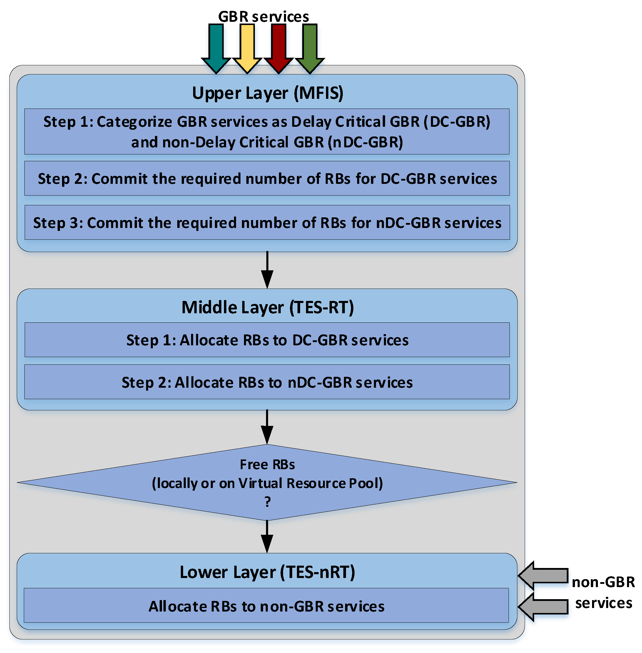
The proposed slicing scheme improves the three-layer design of the FLSA-CC [15] scheduler. In particular, as presented in Figure 1, two service groups are defined, namely the guaranteed bit rate (GBR) and the non-guaranteed bit rate (non-GBR) containing best effort services. Initially, the upper layer categorizes the GBR service flow into two subcategories. The first subcategory called delay critical GBR (DC-GBR) includes services where the observed delay is a very critical factor that should be satisfied. Indicatively, an autonomous navigation service flow with maximum acceptable delay up to 5 ms [39] is considered as a DC-GBR service. Accordingly, the second subcategory called non-delay critical GBR (DC-GBR) includes real-time services with increased tolerance to the delay factor (e.g., conversational video services). Indicatively, a conversational video service flow with maximum acceptable delay up to 150 ms [39] is considered as a nDC-GBR service. Subsequently, the upper layer evaluates the amount of RBs that should be committed for each DC-GBR and nDC-GBR service to satisfy its QoS requirements. Then, the middle layer allocates RBs obtained from the upper layer to both DC-GBR and nDC-GBR services. Finally, the lower layer allocates the remaining RBs to non-GBR services. The functionalities of each layer are described in the following subsections.

3.1.1. The Upper Layer of the Network Slicing Scheme

A set $M_u\left(t_n\right)$ of GBR services per user u requires communication resources to satisfy particular constraints during the $t_n$ TTI. Initially, the upper layer creates two subsets of services, namely the $M_{u,DC-GBR}\left(t_n\right)$ and the $M_{u,nDC-GBR}\left(t_n\right)$ consisting of the DC-GBR and the nDC-GBR services of the user, respectively. Subsequently, for each $m_{u,DC-GBR}\left(t_n\right)\in M_{u,DC-GBR}\left(t_n\right)$ service, the $S_{m,u}^{estimated}\left(t_n\right)$ indicator is defined. It determines the estimated satisfaction grade of user service $m_{u,DC-GBR}$ during the upcoming $t_n$ TTI.

The Mamdani fuzzy inference system (MFIS) system [40] is applied for the estimation of the $S_{m,u}^{estimated}\left(t_n\right)$. In this cases, both the $SIN{R}_{m,u}^{estimated}$ and the $Q_{m,u}^{estimated}$ parameters are considered inputs, while they are expressed as interval valued icosagonal fuzzy numbers (IVIFNs) [6]. The linguistic terms and the corresponding IVIFNs used for the representation of the $S_{m,u}^{estimated}$, the $SIN{R}_{m,u}^{estimated}$ and the $Q_{m,u}^{estimated}$ values are presented in

Table 1. The linguistic terms used for the representation of $M{F}_{SINR}$, $M{F}_Q$ and $M{F}_S$ membership functions and the corresponding interval-valued icosagonal fuzzy numbers.

Linguistic Terms for the ${\mathit{M}\mathit{F}}_{\mathit{S}\mathit{I}\mathit{N}\mathit{R}}$ Membership Functions	Linguistic Terms for the ${\mathit{M}\mathit{F}}_{\mathit{Q}}$ Membership Functions	Linguistic Terms for the ${\mathit{M}\mathit{F}}_{\mathit{S}}$ Membership Functions	Interval-Valued Icosagonal Fuzzy Number
Absolutely Bad (AB)	Absolutely Poor (AP)	Absolutely Unsatisfactory (AU)	[(0, 0, 0, 0, 0, 0, 0, 0, 0, 0, 0.008, 0.023, 0.038, 0.053, 0.068, 0.083, 0.098, 0.113, 0.128, 0.143, 1, 0.20, 0.40, 0.60, 0.80, 0.80, 0.60, 0.40, 0.20), (0, 0, 0, 0, 0, 0, 0, 0, 0, 0, 0.006, 0.018, 0.030, 0.042, 0.054, 0.066, 0.078, 0.090, 0.102, 0.114, 0.8, 0.08, 0.26, 0.44, 0.62, 0.62, 0.44, 0.26, 0.08)]
Too Bad (TB)	Very Poor (VP)	Very Unsatisfactory (VU)	[(0, 0, 0, 0, 0.028, 0.043, 0.058, 0.074, 0.089, 0.104, 0.119, 0.134, 0.149, 0.164, 0.179, 0.194, 0.209, 0.224, 0.239, 0.254, 1, 0.20, 0.40, 0.60, 0.80, 0.80, 0.60, 0.40, 0.20), (0, 0.009, 0.021, 0.033, 0.045, 0.057, 0.069, 0.081, 0.093, 0.105, 0.117, 0.129, 0.141, 0.153, 0.165, 0.177, 0.189, 0.201, 0.213, 0.225, 0.8, 0.08, 0.26, 0.44, 0.62, 0.62, 0.44, 0.26, 0.08)]
Bad (B)	Poor (P)	Unsatisfactory (U)	[(0.079, 0.094, 0.109, 0.124, 0.140, 0.155, 0.170, 0.185, 0.200, 0.215, 0.230, 0.245, 0.260, 0.275, 0.290, 0.305, 0.320, 0.335, 0.350, 0.365, 1, 0.20, 0.40, 0.60, 0.80, 0.80, 0.60, 0.40, 0.20), (0.108, 0.120, 0.132, 0.144, 0.156, 0.168, 0.180, 0.192, 0.204, 0.216, 0.228, 0.240, 0.252, 0.264, 0.276, 0.288, 0.300, 0.312, 0.324, 0.337, 0.8, 0.08, 0.26, 0.44, 0.62, 0.62, 0.44, 0.26, 0.08)]
Less than Enough (LE)	Less than Medium (LM)	Less than Acceptable (LA)	[(0.190, 0.206, 0.221, 0.236, 0.251, 0.266, 0.281, 0.296, 0.311, 0.326, 0.341, 0.356, 0.371, 0.386, 0.401, 0.416, 0.431, 0.446, 0.461, 0.476, 1, 0.20, 0.40, 0.60, 0.80, 0.80, 0.60, 0.40, 0.20), (0.219, 0.231, 0.243, 0.255, 0.267, 0.279, 0.291, 0.303, 0.315, 0.327, 0.339, 0.351, 0.363, 0.375, 0.387, 0.399, 0.412, 0.424, 0.436, 0.448, 0.8, 0.08, 0.26, 0.44, 0.62, 0.62, 0.44, 0.26, 0.08)]
Enough (EN)	Medium (M)	Acceptable (A)	[(0.302, 0.317, 0.332, 0.347, 0.362, 0.377, 0.392, 0.407, 0.422, 0.437, 0.452, 0.467, 0.482, 0.497, 0.512, 0.527, 0.542, 0.557, 0.572, 0.587, 1, 0.20, 0.40, 0.60, 0.80, 0.80, 0.60, 0.40, 0.20), (0.330, 0.342, 0.354, 0.366, 0.378, 0.390, 0.402, 0.414, 0.426, 0.438, 0.450, 0.462, 0.475, 0.487, 0.499, 0.511, 0.523, 0.535, 0.547, 0.559, 0.8, 0.08, 0.26, 0.44, 0.62, 0.62, 0.44, 0.26, 0.08)]
More than Enough (ME)	More than Medium (MM)	More than Acceptable (MA)	[(0.413, 0.428, 0.443, 0.458, 0.473, 0.488, 0.503, 0.518, 0.533, 0.548, 0.563, 0.578, 0.593, 0.608, 0.623, 0.638, 0.653, 0.668, 0.683, 0.698, 1, 0.20, 0.40, 0.60, 0.80, 0.80, 0.60, 0.40, 0.20), (0.441, 0.453, 0.465, 0.477, 0.489, 0.501, 0.513, 0.525, 0.538, 0.550, 0.562, 0.574, 0.586, 0.598, 0.610, 0.622, 0.634, 0.646, 0.658 0.670, 0.8, 0.08, 0.26, 0.44, 0.62, 0.62, 0.44, 0.26, 0.08)]
Less than Excellent (LE)	Less than Good (LG)	Slightly Satisfactory (SS)	[(0.524, 0.539, 0.554, 0.569, 0.584, 0.599, 0.614, 0.629, 0.644, 0.659, 0.674, 0.689, 0.704, 0.719, 0.734, 0.749, 0.764, 0.779, 0.794, 0.810, 1, 0.20, 0.40, 0.60, 0.80, 0.80, 0.60, 0.40, 0.20), (0.552, 0.564, 0.576, 0.588, 0.601, 0.613, 0.625, 0.637, 0.649, 0.661, 0.673, 0.685, 0.697, 0.709, 0.721, 0.733, 0.745, 0.757, 0.769, 0.781, 0.8, 0.08, 0.26, 0.44, 0.62, 0.62, 0.44, 0.26, 0.08)]
Almost Excellent (AE)	Good (G)	Satisfactory (S)	[(0.635, 0.650, 0.665, 0.680, 0.695, 0.710, 0.725, 0.740, 0.755, 0.770, 0.785, 0.800, 0.815, 0.830, 0.845, 0.860, 0.876, 0.891, 0.906, 0.921, 1, 0.20, 0.40, 0.60, 0.80, 0.80, 0.60, 0.40, 0.20), (0.663, 0.676, 0.688, 0.700, 0.712, 0.724, 0.736, 0.748, 0.760, 0.772, 0.784, 0.796, 0.808, 0.820, 0.832, 0.844, 0.856, 0.868, 0.880, 0.892, 0.8, 0.08, 0.26, 0.44, 0.62, 0.62, 0.44, 0.26, 0.08)]
Excellent (EX)	More than Good (MG)	Very Satisfactory (VS)	[(0.746, 0.761, 0.776, 0.791, 0.806, 0.821, 0.836, 0.851, 0.866, 0.881, 0.896, 0.911, 0.926, 0.942, 0.957, 0.972, 0.987, 1, 1, 1, 1, 0.20, 0.40, 0.60, 0.80, 0.80, 0.60, 0.40, 0.20), (0.775, 0.787, 0.799, 0.811, 0.823, 0.835, 0.847, 0.859, 0.871, 0.883, 0.895, 0.907, 0.919, 0.931, 0.943, 0.955, 0.967, 0.979, 0.991, 1, 0.8, 0.08, 0.26, 0.44, 0.62, 0.62, 0.44, 0.26, 0.08)]
Absolutely Excellent (AX)	Absolutely Good (AG)	Absolutely Satisfactory (AS)	[(0.857, 0.872, 0.887, 0.902, 0.917, 0.932, 0.947, 0.962, 0.977, 0.992, 1, 1, 1, 1, 1, 1, 1, 1, 1, 1, 1, 0.20, 0.40, 0.60, 0.80, 0.80, 0.60, 0.40, 0.20), (0.886, 0.898, 0.910, 0.922, 0.934, 0.946, 0.958, 0.970, 0.982, 0.994, 1, 1, 1, 1, 1, 1, 1, 1, 1, 1, 0.8, 0.08, 0.26, 0.44, 0.62, 0.62, 0.44, 0.26, 0.08)]

. In addition,

Table 2. The fuzzy rule (or knowledge) base.

Rule	${\mathit{M}\mathit{F}}_{\mathit{S}\mathit{I}\mathit{N}\mathit{R}}$	Operator	${\mathit{M}\mathit{F}}_{\mathit{Q}}$	${\mathit{M}\mathit{F}}_{\mathit{S}}$
1	AB	and	AP	AU
2	AB	and	VP	AU
3	AB	and	P	AU
4	AB	and	LM	AU
5	AB	and	M	AU
6	AB	and	MM	AU
7	AB	and	LG	AU
8	AB	and	G	AU
9	AB	and	MG	AU
10	AB	and	AG	AU
11	TB	and	AP	AU
12	TB	and	VP	AU
13	TB	and	P	AU
14	TB	and	LM	AU
15	TB	and	M	AU
16	TB	and	MM	VU
17	TB	and	LG	VU
18	TB	and	G	VU
19	TB	and	MG	VU
20	TB	and	AG	VU
21	B	and	AP	AU
22	B	and	VP	AU
23	B	and	P	AU
24	B	and	LM	VU
25	B	and	M	VU
26	B	and	MM	VU
27	B	and	LG	U
28	B	and	G	U
29	B	and	MG	U
30	B	and	AG	U
31	LE	and	AP	AU
32	LE	and	VP	AU
33	LE	and	P	VU
34	LE	and	LM	VU
35	LE	and	M	VU
36	LE	and	MM	U
37	LE	and	LG	U
38	LE	and	G	LA
39	LE	and	MG	LA
40	LE	and	AG	LA
41	EN	and	AP	AU
42	EN	and	VP	AU
43	EN	and	P	VU
44	EN	and	LM	VU
45	EN	and	M	U
46	EN	and	MM	U
47	EN	and	LG	LA
48	EN	and	G	LA
49	EN	and	MG	A
50	EN	and	AG	A
51	ME	and	AP	AU
52	ME	and	VP	VU
53	ME	and	P	VU
54	ME	and	LM	U
55	ME	and	M	U
56	ME	and	MM	LA
57	ME	and	LG	A
58	ME	and	G	A
59	ME	and	MG	MA
60	ME	and	AG	MA
61	LE	and	AP	AU
62	LE	and	VP	VU
63	LE	and	P	U
64	LE	and	LM	U
65	LE	and	M	LA
66	LE	and	MM	A
67	LE	and	LG	A
68	LE	and	G	MA
69	LE	and	MG	SS
70	LE	and	AG	SS
71	AE	and	AP	AU
72	AE	and	VP	VU
73	AE	and	P	U
74	AE	and	LM	LA
75	AE	and	M	LA
76	AE	and	MM	A
77	AE	and	LG	MA
78	AE	and	G	SS
79	AE	and	MG	S
80	AE	and	AG	S
81	EX	and	AP	AU
82	EX	and	VP	VU
83	EX	and	P	U
84	EX	and	LM	LA
85	EX	and	M	A
86	EX	and	MM	MA
87	EX	and	LG	SS
88	EX	and	G	S
89	EX	and	MG	VS
90	EX	and	AG	VS
91	AX	and	AP	AU
92	AX	and	VP	VU
93	AX	and	P	U
94	AX	and	LM	LA
95	AX	and	M	A
96	AX	and	MM	MA
97	AX	and	LG	SS
98	AX	and	G	S
99	AX	and	MG	VS
100	AX	and	AG	AS

presents the fuzzy rules used for the estimation of the $S_{m,u}^{estimated}$ parameter.

In particular, the $SIN{R}_{m,u}^{estimated}$ parameter represents the SINR observed from the user u. Furthermore, the $Q_{m,u}^{estimated}\left(t_n\right)$ parameter represents the estimated quality of the $m_{u,DC-GBR}$ user’s service regarding the available RBs in the $t_n$ TTI. $Q_{m,u}^{estimated}\left(t_n\right)$ is calculated using Formula (1) which applies the multiplicative exponent weighting (MEW) method described in [41]. In this formula, the $t{h}_{m,u}^{estimated}\left(t_n\right)$, the $d_{m,u}^{estimated}\left(t_n\right)$, the $j_{m,u}^{estimated}\left(t_n\right)$ and the $p{l}_{m,u}^{estimated}\left(t_n\right)$ parameters represent the normalized values of the throughput, the packet transfer delay, the jitter and the packet loss ratio parameters, respectively. In addition, the $w_{th}$, $w_d$, $w_j$ and $w_{pl}$ represent the weights of the considered parameters. In this work, the aforementioned weights are calculated using the fuzzy analytic network process (FANP) method [40] which is implemented using IVPFNs:

$$\begin{array}{c}\hfill Q_{m,u}^{estimated}\left(t_n\right)={\left[t{h}_{m,u}^{estimated}\left(t_n\right)\right]}^{w_{th}}·{\left[d_{m,u}^{estimated}\left(t_n\right)\right]}^{w_d}·{\left[j_{m,u}^{estimated}\left(t_n\right)\right]}^{w_j}·{\left[p{l}_{m,u}^{estimated}\left(t_n\right)\right]}^{w_{pl}}\end{array}$$

(1)

Furthermore, it should be noted that the value $t{h}_{m,u}^{estimated}\left(t_n\right)$ is calculated using Formula (2), where $\mu \left(t\right)$ is the estimated throughput per RB and $r^{available}$ represents the number of RBs that are available for allocation:

$$\begin{array}{c}\hfill t{h}_{m,u}^{estimated}\left(t_n\right)=\frac{(\mu \left(t_n\right)·r^{available})-t{h}^{min}}{t{h}^{max}-t{h}^{min}}\end{array}$$

(2)

Moreover, the values of the $d_{m,u}^{estimated}\left(t_n\right)$, $j_{m,u}^{estimated}\left(t_n\right)$ and $p{l}_{m,u}^{estimated}\left(t_n\right)$ parameters are calculated using Formulas (3)–(5), respectively. The $p_{m,u}^{average}$ parameter represents the average packet size, the $d_{m,u}^{past\_average}$ is the past average packet transfer delay and the $t{h}_{m,u}^{required}$ is the required throughput of the $m^{th}$ service of user u:

$$\begin{array}{c}\hfill d_{m,u}^{estimated}\left(t_n\right)=1-\left[\frac{\left(\frac{p_{m,u}^{average}}{t{h}_{m,u}^{estimated}\left(t_n\right)}\right)-d^{min}}{d^{max}-d^{min}}\right]\end{array}$$

(3)

$$\begin{array}{c}\hfill j_{m,u}^{estimated}\left(t_n\right)=1-\left[\frac{|d_{m,u}^{estimated}\left(t_n\right)-d_{m,u}^{past\_average}|-j^{min}}{j^{max}-j^{min}}\right]\end{array}$$

(4)

$$\begin{array}{c}\hfill p{l}_{m,u}^{estimated}\left(t_n\right)=1-\left[\frac{\left(\frac{t{h}_{m,u}^{required}\left(t_n\right)-t{h}_{m,u}^{estimated}\left(t_n\right)}{t{h}_{m,u}^{required}\left(t_n\right)}\right)-p{l}^{min}}{p{l}^{max}-p{l}^{min}}\right]\end{array}$$

(5)

The minimum acceptable satisfaction grades $S_{m,u}^{threshold}$ per user and service are obtained using the $SIN{R}_{m,u}^{threshold}$ and the $Q_{m,u}^{threshold}$ threshold values defined in [39]. Subsequently, the aforementioned procedure is also performed for each $m_{u,nDC-GBR}\left(t_n\right)\in M_{u,nDC-GBR}\left(t_n\right)$ service.

The Mamdani Satisfaction Chart

During the instantiation of the system architecture, a Mamdani satisfaction chart, which contains the $S_{m,u}^{estimated}$ values obtained for each possible $SIN{R}_{m,u}^{estimated}$ and $Q_{m,u}^{estimated}$ combination, is created. Specifically, each satisfaction indicator $S_{m,u}^{estimated}$ of Figure 2 is obtained using the MFIS method, considering the $SIN{R}_{m,u}^{estimated}$ and the $Q_{m,u}^{estimated}$ as input parameters. Both $SIN{R}_{m,u}^{estimated}$ and $Q_{m,u}^{estimated}$ are normalized in order to have values within the range of [0, 1]. In addition, the $M{F}_{SINR}$, $M{F}_Q$, $M{F}_S$ membership functions (MFs) are defined using the equalized universe method (EUM) method [40], indicating the linguistic terms and the corresponding IVPFNs for the fuzzy representation of the $SIN{R}_{m,u}^{estimated}$, $Q_{m,u}^{estimated}$ and $S_{m,u}^{estimated}$ factor, respectively. Thus, for each crisp value, two membership degrees are determined in the corresponding MF, one for the upper octagon and one for the lower octagon. Table 1 represents the linguistic terms and the corresponding IVPFNs of $M{F}_{SINR}$, $M{F}_Q$ and $M{F}_S$ membership functions, which are equally distributed inside the domain [$U_{min},U_{max}$] = [0, 1], as described in [40]. Furthermore, Table 2 presents the considered fuzzy rule base which is used from the MFIS for producing the satisfaction chart.

Indicatively, when the $SIN{R}_{m,u}^{estimated}$ and $Q_{m,u}^{estimated}$ values are too low, the produced $S_{m,u}^{estimated}$ value is too low as well. On the contrary, when the $SIN{R}_{m,u}^{estimated}$ and $Q_{m,u}^{estimated}$ values are close to 1, the produced $S_{m,u}^{estimated}$ value is also high, indicating that the user is fully satisfied. Furthermore, when only one of the $SIN{R}_{m,u}^{estimated}$ or the $Q_{m,u}^{estimated}$ values is close to 0, the user satisfaction is in low levels.

At this point, it has to be noted that since the user’s satisfaction is obtained at the Fog by looking up the performance on the satisfaction indicators’ chart, the overhead introduced is minimal. In addition, the method does not impose any significant overhead at the user equipment due to the monitoring of the $SIN{R}_{m,u}$ and $Q_{m,u}$ parameters.

3.1.2. The Middle Layer of the Network Slicing Scheme

In each TTI, the middle layer allocates to each GBR service the number of RBs estimated from the upper layer. The allocation is performed by applying an improved version of the scheduling metric that the throughput enhanced scheduler (TES) [17] algorithm defines for real-time services, where the maximum acceptable packet loss ratio is considered along with the other parameters that consider the aforementioned metric. Specifically, this metric is calculated using Formula (6), where ${\tau }_i$ stands for the maximum acceptable delay, $DHO{L}_i$ represents the head of line delay, b is a constant, $SIN{R}_i$ represents the signal-to-interference plus noise ratio, $r_i$ is the available throughput and $R_i\left(t\right)$ is the past average throughput for the ith flow. The ${\alpha }_i$ value is calculated using Formula $\left(7\right)$ where ${\delta }_i$ represents the maximum acceptable packet loss ratio:

$$m_{i,k}^{TES-R{T}_{improved}}={\alpha }_i·exp(-\frac{{\tau }_i-DHO{L}_i}{{\tau }_i})·log(b·SIN{R}_i)·\frac{r_i}{R_i\left(t\right)}$$

(6)

$${\alpha }_i=-\frac{log{\delta }_i}{{\tau }_i}$$

(7)

3.1.3. The Lower Layer of the Network Slicing Scheme

The lower layer allocates available RBs to best effort flows using the scheduling metric that the TES [17] algorithm defines for non-real-time services. In particular, the metric is estimated using Formula (8):

$$m_{i,k}^{TES-nRT}={\alpha }_i·DHO{L}_i·log(b·SIN{R}_i)·\frac{r_i}{R_i\left(t\right)}$$

(8)

3.2. The Proposed Network Architecture

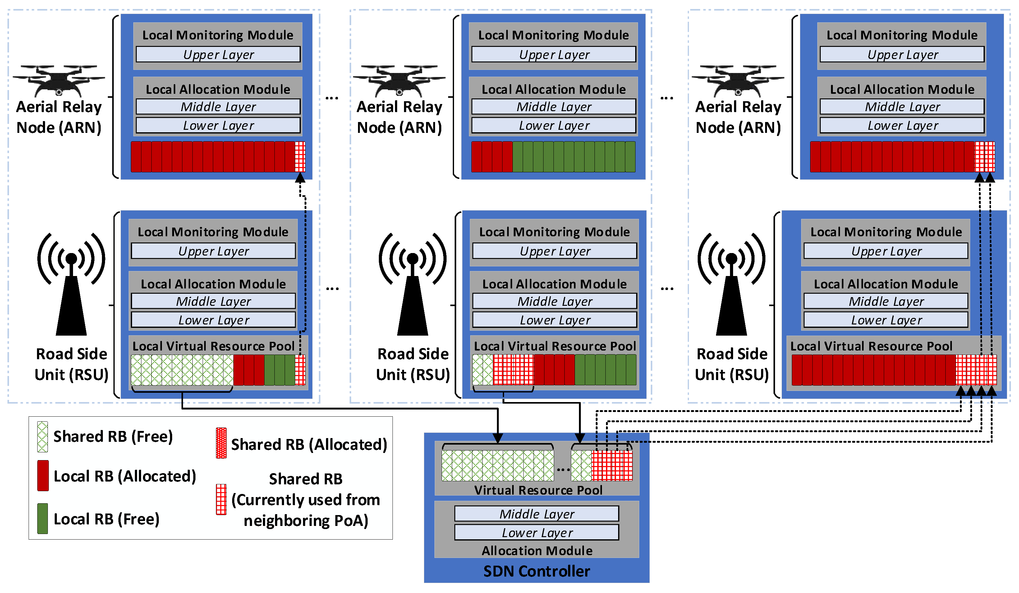
The network architecture (Figure 3) consists ARNs and RSUs that facilitate the provision of network access to vehicular users. In particular, the coverage area of the access network is divided into K cells while each cell is served from an ARN and an RSU.

Each $k\in K$ ARN ($AR{N}_k$) has a local monitoring module (LMM), a local allocation module (LAM) and a set of resource blocks (RBs). A variable $R{B}_{AR{N}_k}^{rem}\left(t_n\right)$ indicates the remaining RBs of the kth ARN during the $t_n$ transmission time interval (TTI). Similarly, each $k\in K$ RSU ($RS{U}_k$) implements its local monitoring module (LMM), its local allocation module (LAM) and a local virtual resource pool (LVRP) with a set of resource blocks (RBs). A variable $R{B}_{RS{U}_k}^{rem}\left(t_n\right)$ indicates the remaining RBs of the kth RSU during the $t_n$ TTI. In addition, the RBs of the LVRP are organized into two subsets, which are called local RBs (LRBs) and shared RBs (SRBs).

An SDN controller maintains a virtual resource pool (VRP) where the SRBs of the RSUs are stored, in a way similar to [36,42]. In addition, the SDN controller includes an allocation module (AM) and a MANO entity which orchestrates the entire network slicing procedure whilst maintaining the necessary frequency reuse factor. At this point, it has to be noted that in order to ensure the scalability of the proposed scheme, multiple SDN controllers can be used. In this case, each SDN controller will maintain a VRP for a specific geographical area in a way similar to that described in [36]. Thus, as the system expands, additional SDN controllers can be used to control the VRPs of each subarea of the entire system coverage.

Based on the layered design of the proposed scheme, the allocation of RBs to user services is as follows. For users of the ARNs, the LMM module of each ARN initially implements the upper layer of the scheme to monitor the satisfaction grade $S_{m,u}^{estimated}\left(t_n\right)$ of each user service. If the estimated $S_{m,u}^{estimated}\left(t_n\right)$ is higher than the predefined $S_{m,u}^{threshold}$ threshold value, the service requirements can be satisfied from the remaining RBs that exist in the current $AR{N}_k$. Thus, the LAM module of the ARN implements the middle and the lower layers of the slicing scheme to allocate RBs of the $AR{N}_k$ to both GBR and non-GBR services for the next TTI. However, if the estimated satisfaction grade $S_{m,u}^{estimated}\left(t_n\right)$ is lower than the predefined $S_{m,u}^{threshold}$ threshold value, the service requirements cannot be satisfied from the $R{B}_{AR{N}_k}^{rem}\left(t_n\right)$. In this case, the ARN borrows extra RBs from the LVRP of the corresponding RSU to achieve the required satisfaction grade. For the users of RSUs, the LMM module of each RSU initially implements the upper layer of the scheme to monitor the satisfaction grade $S_{m,u}^{estimated}\left(t_n\right)$ of each user service. If the remaining RBs of the current $RS{U}_k$ can satisfy the predefined $S_{m,u}^{threshold}$ threshold value, the LAM module of the RSU implements the middle and the lower layers of the slicing scheme to allocate LRBs of the $RS{U}_k$ to both GBR and non-GBR services for the next TTI. The remaining RBs $R{B}_k^{rem}\left(t_n\right)$ are sent back to the VRP of the SDN controller. However, if the remaining RBs of the current $RS{U}_k$ cannot satisfy the $S_{m,u}^{threshold}$ threshold, the AM of the SDN controller implements the middle and the lower layers of the scheme to allocate extra RBs from the VRP to the user services. As far as the VRP is concerned, the algorithm prefers to allocate RBs with similar sub frequencies for each user to minimize the number of antennas required for each vehicle, which is a factor that affects the energy consumption of the system.

4. Optimization of the Positions of ARNs

In this section, an algorithm that optimizes the geographical position of each ARN is described. Using this algorithm, the most appropriate position for each ARN is selected, in order to enhance the overall performance of the system since ARNs with optimized positions provide communication resources with improved channel conditions. More specifically, the main goal of the proposed procedure is the improvement of network technical characteristics such as the throughput, the delay, the jitter and the packet loss ratio, by placing each ARN to the most appropriate position. Indicative criteria that can be considered for this procedure include the vehicle density in each geographical area, the SINR of the corresponding RSU in this area, as well as the average priorities of the services used from the vehicles moving inside this area. Thus, the ARN’s position that maximizes these parameters will be selected.

The Icosagonal Fuzzy TOPSIS (IFT)

As has been proved in several works, the technique for order preference by similarity to ideal solution (TOPSIS) and its variants perform optimal multi-attribute decision making considering multiple criteria. Indicatively, as shown in [43], the trapezoidal fuzzy TOPSIS (TFT) method outperforms the fuzzy analytic hierarchy process (AHP)—elimination et choix traduisant la realité (ELECTRE) [44] method—which is also called FAE method, in scenarios where the most appropriate network should be selected for a user. In addition, as proven in [40], a mobility management scheme that applies the pentagonal fuzzy TOPSIS (PFT) method outperforms the fuzzy AHP simple additive weighting (FAS) [45], the fuzzy AHP multiplicative exponent weighting (FAM) [45] and the FAE methods. Furthermore, similar conclusions about the performance of the TOPSIS method were mentioned to [46,47] against several alternative methodologies. In addition, as it is shown to [48], the trapezoidal fuzzy TOPSIS for heritage route selection (TFT-HRS) method performs the optimal selection of flying routes for drones. By taking into consideration the aforementioned research works, in this paper, the icosagonal fuzzy TOPSIS (IFT) algorithm is proposed for the selection of the optimal positions of the ARNs. It is an improved version of the pentagonal fuzzy TOPSIS (PFT) [40] using interval-valued icosagonal fuzzy numbers for the representations of the values of criteria attributes. As each algorithm that is based on TOPSIS [49], IFT applies the concept that the best alternative solution should have the shortest distance from the positive ideal solution and the longest distance from the negative ideal solution.

Regarding the functionality of the algorithm, a set $C=\{C_1,C_2,\cdots ,C_m\}$ of criteria along with the corresponding criteria weights $w_1,w_2,\cdots ,w_m$ are considered. Furthermore, a list $A=\{A_1,A_2,\cdots ,A_z\}$ is constructed determining the alternative positions from which the best one should be selected for the ARN. The steps of the algorithm are as follows:

• Step 1. Construction of the decision matrix: each $x_{ij}$ element of the $n\times m$ decision matrix D is an interval-valued icosagonal fuzzy number which expresses the evaluation of the alternative position i considering the criterion j. Thus:

  $$D=\begin{array}{cccc}\hfill & \hfill C_1& \hfill \cdots & \hfill C_m\\ \hfill ine{A}_1& \hfill x_{11}& \hfill \cdots & \hfill x_{1m}\\ \hfill ⋮& \hfill ⋮& \hfill \ddots & \hfill ⋮\\ \hfill A_n& \hfill x_{n1}& \hfill \cdots & \hfill x_{nm}\end{array}$$

  (9)

  where: $\begin{array}{c}{x}_{ij}=[(x_{ij1}^U,x_{ij2}^U,x_{ij3}^U,x_{ij4}^U,x_{ij5}^U,x_{ij6}^U,x_{ij7}^U,x_{ij8}^U,x_{ij9}^U,x_{ij10}^U,x_{ij11}^U,x_{ij12}^U,x_{ij13}^U,x_{ij14}^U,x_{ij15}^U,x_{ij16}^U,x_{ij17}^U,x_{ij18}^U,x_{ij19}^U,x_{ij20}^U,v_{ij}^U,v_{ij1}^U,v_{ij2}^U,v_{ij3}^U,v_{ij4}^U,v_{ij5}^U,v_{ij6}^U,v_{ij7}^U,v_{ij8}^U,\\ x_{ij1}^L,x_{ij2}^L,x_{ij3}^L,x_{ij4}^L,x_{ij5}^L,x_{ij6}^L,x_{ij7}^L,x_{ij8}^L,x_{ij9}^L,x_{ij10}^L,x_{ij11}^L,x_{ij12}^L,x_{ij13}^L,x_{ij14}^L,x_{ij15}^L,x_{ij16}^L,x_{ij17}^L,x_{ij18}^L,x_{ij19}^L,x_{ij20}^L,v_{ij}^L,v_{ij1}^L,v_{ij2}^L,v_{ij3}^L,v_{ij4}^L,v_{ij5}^L,v_{ij6}^L,v_{ij7}^L,v_{ij8}^L)]\end{array}$.
• Step 2. Normalization of the decision matrix: consider that ${\Omega }_b$ is the set of benefit evaluation criteria and ${\Omega }_c$ is the set of cost evaluation criteria. Then, the elements of the normalized decision matrix are computed as

  $$\begin{array}{c}{r}_{ij}=\left[\right(\frac{x_{ij1}^U}{b_j},\frac{x_{ij2}^U}{b_j},\frac{x_{ij3}^U}{b_j},\frac{x_{ij4}^U}{b_j},\frac{x_{ij5}^U}{b_j},\frac{x_{ij6}^U}{b_j},\frac{x_{ij7}^U}{b_j},\frac{x_{ij8}^U}{b_j},\frac{x_{ij9}^U}{b_j},\frac{x_{ij10}^U}{b_j},\frac{x_{ij11}^U}{b_j},\frac{x_{ij12}^U}{b_j},\frac{x_{ij13}^U}{b_j},\frac{x_{ij14}^U}{b_j},\frac{x_{ij15}^U}{b_j},\\ \frac{x_{ij16}^U}{b_j},\frac{x_{ij17}^U}{b_j},\frac{x_{ij18}^U}{b_j},\frac{x_{ij19}^U}{b_j},\frac{x_{ij20}^U}{b_j},v_{ij}^U,v_{ij1}^U,v_{ij2}^U,v_{ij3}^U,v_{ij4}^U,v_{ij5}^U,v_{ij6}^U,v_{ij7}^U,v_{ij8}^U),\\ (\frac{x_{ij1}^L}{b_j},\frac{x_{ij2}^L}{b_j},\frac{x_{ij3}^L}{b_j},\frac{x_{ij4}^L}{b_j},\frac{x_{ij5}^L}{b_j},\frac{x_{ij6}^L}{b_j},\frac{x_{ij7}^L}{b_j},\frac{x_{ij8}^L}{b_j},\frac{x_{ij9}^L}{b_j},\frac{x_{ij10}^L}{b_j},\frac{x_{ij11}^L}{b_j},\frac{x_{ij12}^L}{b_j},\frac{x_{ij13}^L}{b_j},\frac{x_{ij14}^L}{b_j},\frac{x_{ij15}^L}{b_j},\\ \frac{x_{ij16}^L}{b_j},\frac{x_{ij17}^L}{b_j},\frac{x_{ij18}^L}{b_j},\frac{x_{ij19}^L}{b_j},\frac{x_{ij20}^L}{b_j},v_{ij}^L,v_{ij1}^L,v_{ij2}^L,v_{ij3}^L,v_{ij4}^L,v_{ij5}^L,v_{ij6}^L,v_{ij7}^L,v_{ij8}^L\left)\right]\end{array}$$

  (10)

  where $b_j={max}_i{x}_{ij}^U$ for each $j\in {\Omega }_b$, or:

  $$\begin{array}{c}{r}_{ij}=\left[\right(\frac{c_j}{x_{ij1}^U},\frac{c_j}{x_{ij2}^U},\frac{c_j}{x_{ij3}^U},\frac{c_j}{x_{ij4}^U},\frac{c_j}{x_{ij5}^U},\frac{c_j}{x_{ij6}^U},\frac{c_j}{x_{ij7}^U},\frac{c_j}{x_{ij8}^U},\frac{c_j}{x_{ij9}^U},\frac{c_j}{x_{ij10}^U},\frac{c_j}{x_{ij11}^U},\frac{c_j}{x_{ij12}^U},\frac{c_j}{x_{ij13}^U},\frac{c_j}{x_{ij14}^U},\frac{c_j}{x_{ij15}^U},\\ \frac{c_j}{x_{ij16}^U},\frac{c_j}{x_{ij17}^U},\frac{c_j}{x_{ij18}^U},\frac{c_j}{x_{ij19}^U},\frac{c_j}{x_{ij20}^U},v_{ij}^U,v_{ij1}^U,v_{ij2}^U{v}_{ij3}^U,v_{ij4}^U,v_{ij5}^U,v_{ij6}^U,v_{ij7}^U,v_{ij8}^U),\\ (\frac{c_j}{x_{ij1}^L},\frac{c_j}{x_{ij2}^L},\frac{c_j}{x_{ij3}^L},\frac{c_j}{x_{ij4}^L},\frac{c_j}{x_{ij5}^L},\frac{c_j}{x_{ij6}^L},\frac{c_j}{x_{ij7}^L},\frac{c_j}{x_{ij8}^L},\frac{c_j}{x_{ij9}^L},\frac{c_j}{x_{ij10}^L},\frac{c_j}{x_{ij11}^L},\frac{c_j}{x_{ij12}^L},\frac{c_j}{x_{ij13}^L},\frac{c_j}{x_{ij14}^L},\frac{c_j}{x_{ij15}^L},\\ \frac{c_j}{x_{ij16}^L},\frac{c_j}{x_{ij17}^L},\frac{c_j}{x_{ij18}^L},\frac{c_j}{x_{ij19}^L},\frac{c_j}{x_{ij20}^L},v_{ij}^L,v_{ij1}^L,v_{ij2}^L,v_{ij3}^L,v_{ij4}^L,v_{ij5}^L,v_{ij6}^L,v_{ij7}^L,v_{ij8}^L\left)\right]\end{array}$$

  (11)

  where $c_j={min}_i{x}_{ij}^L$ for each $j\in {\Omega }_c$.
• Step 3. Construction of the weighted normalized decision matrix: for the construction of the weighted normalized decision matrix, each element $r_{ij}$ of the normalized decision matrix is multiplied with the respective criterion weight $w_j$ according to the formula:

  $$\begin{array}{c}{u}_{ij}=\left[\right(r_{ij1}^U·w_j,r_{ij2}^U·w_j,r_{ij3}^U·w_j,r_{ij4}^U·w_j,r_{ij5}^U·w_j,r_{ij6}^U·w_j,r_{ij7}^U·w_j,r_{ij8}^U·w_j,r_{ij9}^U·w_j,\\ r_{ij10}^U·w_j,r_{ij11}^U·w_j,r_{ij12}^U·w_j,r_{ij13}^U·w_j,r_{ij14}^U·w_j,r_{ij15}^U·w_j,r_{ij16}^U·w_j,r_{ij17}^U·w_j,r_{ij18}^U·w_j,\\ r_{ij19}^U·w_j,r_{ij20}^U·w_j,v_{ij}^U,v_{ij1}^U,v_{ij2}^U,v_{ij3}^U,v_{ij4}^U,v_{ij5}^U,v_{ij6}^U,v_{ij7}^U,v_{ij8}^U),\\ (r_{ij1}^L·w_j,r_{ij2}^L·w_j,r_{ij3}^L·w_j,r_{ij4}^L·w_j,r_{ij5}^L·w_j,r_{ij6}^L·w_j,r_{ij7}^L·w_j,r_{ij8}^L·w_j,r_{ij9}^L·\\ w_j,r_{ij10}^L·w_j,r_{ij11}^L·w_j,r_{ij12}^L·w_j,r_{ij13}^L·w_j,r_{ij14}^L·w_j,r_{ij15}^L·w_j,r_{ij16}^L·w_j,r_{ij17}^L·w_j,r_{ij18}^L·\\ w_j,r_{ij19}^L·w_j,r_{ij20}^L·w_j,v_{ij}^L,v_{ij1}^L,v_{ij2}^L,v_{ij3}^L,v_{ij4}^L,v_{ij5}^L,v_{ij6}^L,v_{ij7}^L,v_{ij8}^L\left)\right]\end{array}$$

  (12)
  At this point, it must be noted that the criteria weights can be estimated using the analytic hierarchy process (AHP) [50], the analytic network process (ANP) [51] or another similar method.
• Step 4. Determination of the positive and negative ideal solution: in this step, the positive ideal solution is defined as

  $$\begin{array}{c}{X}^{+}=\left[\right(x_{ij1}^{+U},x_{ij2}^{+U},x_{ij3}^{+U},x_{ij4}^{+U},x_{ij5}^{+U},x_{ij6}^{+U},x_{ij7}^{+U},x_{ij8}^{+U},x_{ij9}^{+U},x_{ij10}^{+U},x_{ij11}^{+U},x_{ij12}^{+U},x_{ij13}^{+U},x_{ij14}^{+U},x_{ij15}^{+U},\hfill \\ x_{ij16}^{+U},x_{ij17}^{+U},x_{ij18}^{+U},x_{ij19}^{+U},x_{ij20}^{+U},v_{ij}^{+U},v_{ij1}^{+U},v_{ij2}^{+U},v_{ij3}^{+U},v_{ij4}^{+U},v_{ij5}^{+U},v_{ij6}^{+U},v_{ij7}^{+U},v_{ij8}^{+U}),\\ (x_{ij1}^{+L},x_{ij2}^{+L},x_{ij3}^{+L},x_{ij4}^{+L},x_{ij5}^{+L},x_{ij6}^{+L},x_{ij7}^{+L},x_{ij8}^{+L},x_{ij9}^{+L},x_{ij10}^{+L},x_{ij11}^{+L},x_{ij12}^{+L},x_{ij13}^{+L},x_{ij14}^{+L},x_{ij15}^{+L},\\ x_{ij16}^{+L},x_{ij17}^{+L},x_{ij18}^{+L},x_{ij19}^{+L},x_{ij20}^{+L},v_{ij}^{+L},v_{ij1}^{+L},v_{ij2}^{+L},v_{ij3}^{+L},v_{ij4}^{+L},v_{ij5}^{+L},v_{ij6}^{+L},v_{ij7}^{+L},v_{ij8}^{+L}\left)\right]=\\ [(\underset{i}{\bigwedge }{u}_{ij1}^U,\underset{i}{\bigwedge }{u}_{ij2}^U,\underset{i}{\bigwedge }{u}_{ij3}^U,\underset{i}{\bigwedge }{u}_{ij4}^U,\underset{i}{\bigwedge }{u}_{ij5}^U,\underset{i}{\bigwedge }{u}_{ij6}^U,\underset{i}{\bigwedge }{u}_{ij7}^U,\underset{i}{\bigwedge }{u}_{ij8}^U,\underset{i}{\bigwedge }{u}_{ij9}^U,\underset{i}{\bigwedge }{u}_{ij10}^U,\\ \underset{i}{\bigwedge }{u}_{ij11}^U,\underset{i}{\bigwedge }{u}_{ij12}^U,\underset{i}{\bigwedge }{u}_{ij13}^U,\underset{i}{\bigwedge }{u}_{ij14}^U,\underset{i}{\bigwedge }{u}_{ij15}^U,\underset{i}{\bigwedge }{u}_{ij16}^U,\underset{i}{\bigwedge }{u}_{ij17}^U,\underset{i}{\bigwedge }{u}_{ij18}^U,\underset{i}{\bigwedge }{u}_{ij19}^U,\underset{i}{\bigwedge }{u}_{ij20}^U,\\ v_{ij}^U,v_{ij1}^U,v_{ij2}^U,v_{ij3}^U,v_{ij4}^U,v_{ij5}^U,v_{ij6}^U,v_{ij7}^U,v_{ij8}^U),\\ (\underset{i}{\bigwedge }{u}_{ij1}^L,\underset{i}{\bigwedge }{u}_{ij2}^L,\underset{i}{\bigwedge }{u}_{ij3}^L,\underset{i}{\bigwedge }{u}_{ij4}^L,\underset{i}{\bigwedge }{u}_{ij5}^L,\underset{i}{\bigwedge }{u}_{ij6}^L,\underset{i}{\bigwedge }{u}_{ij7}^L,\underset{i}{\bigwedge }{u}_{ij8}^L,\underset{i}{\bigwedge }{u}_{ij9}^L,\underset{i}{\bigwedge }{u}_{ij10}^L,\\ \underset{i}{\bigwedge }{u}_{ij11}^L,\underset{i}{\bigwedge }{u}_{ij12}^L,\underset{i}{\bigwedge }{u}_{ij13}^L,\underset{i}{\bigwedge }{u}_{ij14}^L,\underset{i}{\bigwedge }{u}_{ij15}^L,\underset{i}{\bigwedge }{u}_{ij16}^L,\underset{i}{\bigwedge }{u}_{ij17}^L,\underset{i}{\bigwedge }{u}_{ij18}^L,\underset{i}{\bigwedge }{u}_{ij19}^L,\underset{i}{\bigwedge }{u}_{ij20}^L,\\ v_{ij}^L,v_{ij1}^L,v_{ij2}^L,v_{ij3}^L,v_{ij4}^L,v_{ij5}^L,v_{ij6}^L,v_{ij7}^L,v_{ij8}^L\left)\right]\end{array}$$

  (13)

  where $\underset{i}{\bigwedge }\equiv {max}_i$ in case $j\in {\Omega }_b$ and $\underset{i}{\bigwedge }\equiv {min}_i$ in case $j\in {\Omega }_c$. Accordingly, the negative ideal solutions is defined as

  $$\begin{array}{c}{X}^{-}=\left[\right(x_{ij1}^{-U},x_{ij2}^{-U},x_{ij3}^{-U},x_{ij4}^{-U},x_{ij5}^{-U},x_{ij6}^{-U},x_{ij7}^{-U},x_{ij8}^{-U},x_{ij9}^{-U},x_{ij10}^{-U},x_{ij11}^{-U},x_{ij12}^{-U},x_{ij13}^{-U},x_{ij14}^{-U},x_{ij15}^{-U},\hfill \\ x_{ij16}^{-U},x_{ij17}^{-U},x_{ij18}^{-U},x_{ij19}^{-U},x_{ij20}^{-U},v_{ij}^{-U},v_{ij1}^{-U},v_{ij2}^{-U},v_{ij3}^{-U},v_{ij4}^{-U},v_{ij5}^{-U},v_{ij6}^{-U},v_{ij7}^{-U},v_{ij8}^{-U}),\\ (x_{ij1}^{-L},x_{ij2}^{-L},x_{ij3}^{-L},x_{ij4}^{-L},x_{ij5}^{-L},x_{ij6}^{-L},x_{ij7}^{-L},x_{ij8}^{-L},x_{ij9}^{-L},x_{ij10}^{-L},x_{ij11}^{-L},x_{ij12}^{-L},x_{ij13}^{-L},x_{ij14}^{-L},x_{ij15}^{-L},\\ x_{ij16}^{-L},x_{ij17}^{-L},x_{ij18}^{-L},x_{ij19}^{-L},x_{ij20}^{-L},v_{ij}^{-L},v_{ij1}^{-L},v_{ij2}^{-L},v_{ij3}^{-L},v_{ij4}^{-L},v_{ij5}^{-L},v_{ij6}^{-L},v_{ij7}^{-L},v_{ij8}^{-L}\left)\right]=\\ [(\underset{i}{\bigwedge }{u}_{ij1}^U,\underset{i}{\bigwedge }{u}_{ij2}^U,\underset{i}{\bigwedge }{u}_{ij3}^U,\underset{i}{\bigwedge }{u}_{ij4}^U,\underset{i}{\bigwedge }{u}_{ij5}^U,\underset{i}{\bigwedge }{u}_{ij6}^U,\underset{i}{\bigwedge }{u}_{ij7}^U,\underset{i}{\bigwedge }{u}_{ij8}^U,\underset{i}{\bigwedge }{u}_{ij9}^U,\underset{i}{\bigwedge }{u}_{ij10}^U,\\ \underset{i}{\bigwedge }{u}_{ij11}^U,\underset{i}{\bigwedge }{u}_{ij12}^U,\underset{i}{\bigwedge }{u}_{ij13}^U,\underset{i}{\bigwedge }{u}_{ij14}^U,\underset{i}{\bigwedge }{u}_{ij15}^U,\underset{i}{\bigwedge }{u}_{ij16}^U,\underset{i}{\bigwedge }{u}_{ij17}^U,\underset{i}{\bigwedge }{u}_{ij18}^U,\underset{i}{\bigwedge }{u}_{ij19}^U,\underset{i}{\bigwedge }{u}_{ij20}^U,\\ v_{ij}^U,v_{ij1}^U,v_{ij2}^U,v_{ij3}^U,v_{ij4}^U,v_{ij5}^U,v_{ij6}^U,v_{ij7}^U,v_{ij8}^U),\\ (\underset{i}{\bigwedge }{u}_{ij1}^L,\underset{i}{\bigwedge }{u}_{ij2}^L,\underset{i}{\bigwedge }{u}_{ij3}^L,\underset{i}{\bigwedge }{u}_{ij4}^L,\underset{i}{\bigwedge }{u}_{ij5}^L,\underset{i}{\bigwedge }{u}_{ij6}^L,\underset{i}{\bigwedge }{u}_{ij7}^L,\underset{i}{\bigwedge }{u}_{ij8}^L,\underset{i}{\bigwedge }{u}_{ij9}^L,\underset{i}{\bigwedge }{u}_{ij10}^L,\\ \underset{i}{\bigwedge }{u}_{ij11}^L,\underset{i}{\bigwedge }{u}_{ij12}^L,\underset{i}{\bigwedge }{u}_{ij13}^L,\underset{i}{\bigwedge }{u}_{ij14}^L,\underset{i}{\bigwedge }{u}_{ij15}^L,\underset{i}{\bigwedge }{u}_{ij16}^L,\underset{i}{\bigwedge }{u}_{ij17}^L,\underset{i}{\bigwedge }{u}_{ij18}^L,\underset{i}{\bigwedge }{u}_{ij19}^L,\underset{i}{\bigwedge }{u}_{ij20}^L,\\ v_{ij}^L,v_{ij1}^L,v_{ij2}^L,v_{ij3}^L,v_{ij4}^L,v_{ij5}^L,v_{ij6}^L,v_{ij7}^L,v_{ij8}^L\left)\right]\end{array}$$

  (14)

  where ${\bigvee }_i\equiv {min}_i$ in case $j\in {\Omega }_b$ and ${\bigvee }_i\equiv {max}_i$ in case $j\in {\Omega }_c$.
• Step 5. Estimation of the distance of each alternative solution from the positive and the negative ideal solutions: the distances $d_{i1}^{+}$ and $d_{i2}^{+}$ of each alternative solution from the positive ideal solution are estimated as follows:

  $$\begin{array}{c}{d}_{i1}^{+}=\sum _{j=1}^m\{\frac{1}{20}[{(u_{ij1}^U-x_{ij1}^{+U})}^2+{(u_{ij2}^U-x_{ij2}^{+U})}^2+{(u_{ij3}^U-x_{ij3}^{+U})}^2+{(u_{ij4}^U-x_{ij4}^{+U})}^2\hfill \\ \hspace{1em} +{(u_{ij5}^U-x_{ij5}^{+U})}^2+{(u_{ij6}^U-x_{ij6}^{+U})}^2+{(u_{ij7}^U-x_{ij7}^{+U})}^2+{(u_{ij8}^U-x_{ij8}^{+U})}^2\\ \hspace{1em} +{(u_{ij9}^U-x_{ij9}^{+U})}^2+{(u_{ij10}^U-x_{ij10}^{+U})}^2+{(u_{ij11}^U-x_{ij11}^{+U})}^2+{(u_{ij12}^U-x_{ij12}^{+U})}^2\\ \hspace{1em} +{(u_{ij13}^U-x_{ij13}^{+U})}^2+{(u_{ij14}^U-x_{ij14}^{+U})}^2+{(u_{ij15}^U-x_{ij15}^{+U})}^2+{(u_{ij16}^U-x_{ij16}^{+U})}^2\\ \hfill \hspace{1em} +{(u_{ij17}^U-x_{ij17}^{+U})}^2+{(u_{ij18}^U-x_{ij18}^{+U})}^2+{(u_{ij19}^U-x_{ij19}^{+U})}^2+{(u_{ij20}^U-x_{ij20}^{+U})}^2{\left]\right\}}^{\frac{1}{2}}\end{array}$$

  (15)

  $$\begin{array}{c}{d}_{i2}^{+}=\sum _{j=1}^m\{\frac{1}{20}[{(u_{ij1}^L-x_{ij1}^{+L})}^2+{(u_{ij2}^L-x_{ij2}^{+L})}^2+{(u_{ij3}^L-x_{ij3}^{+L})}^2+{(u_{ij4}^L-x_{ij4}^{+L})}^2\hfill \\ \hspace{1em} +{(u_{ij5}^L-x_{ij5}^{+L})}^2+{(u_{ij6}^L-x_{ij6}^{+L})}^2+{(u_{ij7}^L-x_{ij7}^{+L})}^2+{(u_{ij8}^L-x_{ij8}^{+L})}^2\\ \hspace{1em} +{(u_{ij9}^L-x_{ij9}^{+L})}^2+{(u_{ij10}^L-x_{ij10}^{+L})}^2+{(u_{ij11}^L-x_{ij11}^{+L})}^2+{(u_{ij12}^L-x_{ij12}^{+L})}^2\\ \hspace{1em} +{(u_{ij13}^L-x_{ij13}^{+L})}^2+{(u_{ij14}^L-x_{ij14}^{+L})}^2+{(u_{ij15}^L-x_{ij15}^{+L})}^2+{(u_{ij16}^L-x_{ij16}^{+L})}^2\\ \hfill \hspace{1em} +{(u_{ij17}^L-x_{ij17}^{+L})}^2+{(u_{ij18}^L-x_{ij18}^{+L})}^2+{(u_{ij19}^L-x_{ij19}^{+L})}^2+{(u_{ij20}^L-x_{ij20}^{+L})}^2{\left]\right\}}^{\frac{1}{2}}\end{array}$$

  (16)

  Similarly, the distances $d_{i1}^{-}$ and $d_{i2}^{-}$ of each alternative solution from the negative ideal solution are estimated as follows:

  $$\begin{array}{c}{d}_{i1}^{-}=\sum _{j=1}^m\{\frac{1}{20}[{(u_{ij1}^U-x_{ij1}^{-U})}^2+{(u_{ij2}^U-x_{ij2}^{-U})}^2+{(u_{ij3}^U-x_{ij3}^{-U})}^2+{(u_{ij4}^U-x_{ij4}^{-U})}^2\hfill \\ \hspace{1em} +{(u_{ij5}^U-x_{ij5}^{-U})}^2+{(u_{ij6}^U-x_{ij6}^{-U})}^2+{(u_{ij7}^U-x_{ij7}^{-U})}^2+{(u_{ij8}^U-x_{ij8}^{-U})}^2\\ \hspace{1em} +{(u_{ij9}^U-x_{ij9}^{-U})}^2+{(u_{ij10}^U-x_{ij10}^{-U})}^2+{(u_{ij11}^U-x_{ij11}^{-U})}^2+{(u_{ij12}^U-x_{ij12}^{-U})}^2\\ \hspace{1em} +{(u_{ij13}^U-x_{ij13}^{-U})}^2+{(u_{ij14}^U-x_{ij14}^{-U})}^2+{(u_{ij15}^U-x_{ij15}^{-U})}^2+{(u_{ij16}^U-x_{ij16}^{-U})}^2\\ \hfill \hspace{1em} +{(u_{ij17}^U-x_{ij17}^{-U})}^2+{(u_{ij18}^U-x_{ij18}^{-U})}^2+{(u_{ij19}^U-x_{ij19}^{-U})}^2+{(u_{ij20}^U-x_{ij20}^{-U})}^2{\left]\right\}}^{\frac{1}{2}}\end{array}$$

  (17)

  $$\begin{array}{c}{d}_{i2}^{-}=\sum _{j=1}^m\{\frac{1}{20}[{(u_{ij1}^L-x_{ij1}^{-L})}^2+{(u_{ij2}^L-x_{ij2}^{-L})}^2+{(u_{ij3}^L-x_{ij3}^{-L})}^2+{(u_{ij4}^L-x_{ij4}^{-L})}^2\hfill \\ \hspace{1em} +{(u_{ij5}^L-x_{ij5}^{-L})}^2+{(u_{ij6}^L-x_{ij6}^{-L})}^2+{(u_{ij7}^L-x_{ij7}^{-L})}^2+{(u_{ij8}^L-x_{ij8}^{-L})}^2\\ \hspace{1em} +{(u_{ij9}^L-x_{ij9}^{-L})}^2+{(u_{ij10}^L-x_{ij10}^{-L})}^2+{(u_{ij11}^L-x_{ij11}^{-L})}^2+{(u_{ij12}^L-x_{ij12}^{-L})}^2\\ \hspace{1em} +{(u_{ij13}^L-x_{ij13}^{-L})}^2+{(u_{ij14}^L-x_{ij14}^{-L})}^2+{(u_{ij15}^L-x_{ij15}^{-L})}^2+{(u_{ij16}^L-x_{ij16}^{-L})}^2\\ \hfill \hspace{1em} +{(u_{ij17}^L-x_{ij17}^{-L})}^2+{(u_{ij18}^L-x_{ij18}^{-L})}^2+{(u_{ij19}^L-x_{ij19}^{-L})}^2+{(u_{ij20}^L-x_{ij20}^{-L})}^2{\left]\right\}}^{\frac{1}{2}}\end{array}$$

  (18)

  Thus, the distance of the alternative solutions from the positive and negative ideal solutions are expressed by intervals such as $[d_{i1}^{+},d_{i2}^{+}]$ and $[d_{i1}^{-},d_{i2}^{-}]$ [52], instead of single values. In this way, less information is lost.
• Step 6. Calculation of the relative closeness: the relative closeness of the distances from the ideal solutions are computed as follows:

  $$R{C}_{i1}=\frac{d_{i1}^{-}}{d_{i1}^{+}+d_{i1}^{-}}$$

  (19)

  and:

  $$R{C}_{i2}=\frac{d_{i2}^{-}}{d_{i2}^{+}+d_{i2}^{-}}$$

  (20)

  The compound relative closeness is obtained from the average of the above values:

  $$R{C}_i=\frac{R{C}_{i1}+R{C}_{i2}}{2}$$

  (21)
• Step 7. Alternatives ranking: the alternative solutions are ranked according to their $R{C}_i$ values. The position with the higher $R{C}_i$ value is selected since it is considered the best alternative solution.

5. Simulation Setup

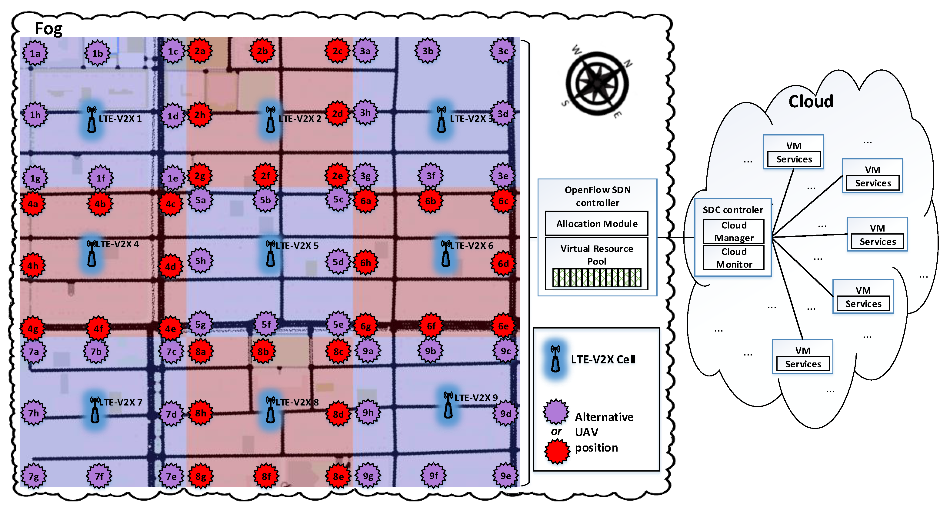
For the evaluation of the proposed scheme, the UAV-aided 5G network topology presented in Figure 4 is simulated. A map of the area where the University of Piraeus is located has been created using the open street map (OSM) software [53]. Then, the map has been used as input in the simulator of urban mobility (SUMO) simulator [54] allowing the production of a trace file indicating the mobility of vehicles in the corresponding geographical area. At this point, it has to be noted that the average height of the buildings that exist to the simulated map, is supposed to be equal to 30 m. Subsequently, the network topology is being built upon the map, using the Network Simulator 3 (NS3) [55], including a Fog and a Cloud infrastructure.

The Fog infrastructure consists of nine LTE-V2X RSUs, along with an ARN per LTE-V2X RSU providing additional communication resources for users moving inside the corresponding coverage area. Both the medium access control (MAC) and the physical (PHY) layers of the LTE-V2X RSUs and ARNs are simulated using the LTE-V2X extension module of the NS3 [56]. In addition, the default altitude of each ARN is equal to the average height of the buildings that exist on the map.

Table 3. The spectrum used from each RSU and ARN.

Name	Uplink Spectrum		Downlink Spectrum		LTE Band Number
	From	To	From	To
LTE-V2X 1	703 MHz	723 MHz	758 MHz	778 MHz	28
LTE-V2X 2	832 MHz	852 MHz	800 MHz	820 MHz	20
LTE-V2X 3	1630 MHz	1650 MHz	1525 MHz	1545 MHz	24
LTE-V2X 4	1710 MHz	1730 MHz	1805 MHz	1825 MHz	3
LTE-V2X 5	1730 MHz	1750 MHz	1825 MHz	1845 MHz	3
LTE-V2X 6	1750 MHz	1770 MHz	1845 MHz	1865 MHz	3
LTE-V2X 7	1900 MHz	1920 MHz	2600 MHz	2620 MHz	15
LTE-V2X 8	1920 MHz	1940 MHz	2110 MHz	2130 MHz	1
LTE-V2X 9	1940 MHz	1960 MHz	2130 MHz	2150 MHz	1
ARN 1	1960 MHz	1980 MHz	2150 MHz	2170 MHz	1
ARN 2	2000 MHz	2020 MHz	2180 MHz	2200 MHz	23
ARN 3	2500 MHz	2520 MHz	2620 MHz	2640 MHz	7
ARN 4	2520 MHz	2540 MHz	2640 MHz	2660 MHz	7
ARN 5	2540 MHz	2560 MHz	2660 MHz	2680 MHz	7
ARN 6	3410 MHz	3430 MHz	3510 MHz	3530 MHz	22
ARN 7	3430 MHz	3450 MHz	3530 MHz	3550 MHz	22
ARN 8	3450 MHz	3470 MHz	3550 MHz	3570 MHz	22
ARN 9	3470 MHz	3490 MHz	3570 MHz	3590 MHz	22

presents the spectrum used from each RSU and ARN, while

Table 4. The geographical position of each RSU and ARN.

RSU	Geographic Latitude, Geographic Longitude
LTE-V2X 1	37.941746, 23.647962
LTE-V2X 2	37.942985, 23.649007
LTE-V2X 3	37.944259, 23.650166
LTE-V2X 4	37.941141, 23.649080
LTE-V2X 5	37.942303, 23.650272
LTE-V2X 6	37.943664, 23.651470
LTE-V2X 7	37.940304, 23.650710
LTE-V2X 8	37.941564, 23.651784
LTE-V2X 9	37.942847, 23.652859
ARN	Possible Position: Geographic Latitude, Geographic Longitude
ARN 1	1a: 37.941630, 23.646994 - 1b: 37.942107, 23.647428 - 1c: 37.942617, 23.647842 - 1d: 37.942334, 23.648342 1e: 37.941989, 23.648996 - 1f: 37.941489, 23.648520 - 1g: 37.941061, 23.648098 - 1h: 37.941347, 23.647473
ARN 2	2a: 37.942795, 23.647994 - 2b: 37.943256, 23.648375 - 2c: 37.943846, 23.648896 - 2d: 37.942317, 23.648341 2e: 37.943244, 23.650030 - 2f: 37.942758, 23.649617 - 2g: 37.942224, 23.649160 - 2h: 37.942592, 23.648570
ARN 3	3a: 37.944008, 23.649037 - 3b: 37.944502, 23.649430 - 3c: 37.945053, 23.649887 - 3d: 37.944801, 23.650429 3e: 37.944441, 23.651041 - 3f: 37.943850, 23.650572 - 3g: 37.943340, 23.650169 - 3h: 37.943895, 23.649658
ARN 4	4a: 37.940950, 23.648250 - 4b: 37.941363, 23.648619 - 4c: 37.941887, 23.649127 - 4d: 37.941560, 23.649751 4e: 37.941251, 23.650302 - 4f: 37.940781, 23.649910 - 4g: 37.940312, 23.649487 - 4h: 37.940622, 23.648926
ARN 5	5a: 37.942098, 23.649270 - 5b: 37.942664, 23.649770 - 5c: 37.943085, 23.650107 - 5d: 37.942806, 23.650774 5e: 37.942424, 23.651281 - 5f: 37.941937, 23.650920 - 5g: 37.941428, 23.650485 - 5h: 37.941747, 23.649841
ARN 6	6a: 37.943197, 23.650268 - 6b: 37.943756, 23.650725 - 6c: 37.944339, 23.651194 - 6d: 37.944011, 23.651859 6e: 37.943743, 23.652401 - 6f: 37.943079, 23.651867 - 6g: 37.942682, 23.651530 - 6h: 37.943041, 23.650980
ARN 7	7a: 37.940158, 23.649763 - 7b: 37.940619, 23.650154 - 7c: 37.941137, 23.650589 - 7d: 37.940896, 23.651039 7e: 37.940459, 23.651762 - 7f: 37.940014, 23.651017 - 7g: 37.939674, 23.650724 - 7h: 37.939901, 23.650201
ARN 8	8a: 37.941282, 23.650730 - 8b: 37.941817, 23.651155 - 8c: 37.942236, 23.651555 - 8d: 37.942084, 23.652112 8e: 37.941714, 23.652786 - 8f: 37.941344, 23.652356 - 8g: 37.940726, 23.651990 - 8h: 37.941091, 23.651150
ARN 9	9a: 37.942586, 23.651776 - 9b: 37.942974, 23.652134 - 9c: 37.943596, 23.652687 - 9d: 37.943346, 23.653167 9e: 37.942959, 23.653872 - 9f: 37.942377, 23.653362 - 9g: 37.941902, 23.652866 - 9h: 37.942278, 23.652275

presents their geographical positions. Also, an OpenFlow SDN controller provides centralized control of the entire network access environment. The 3GPP urban channel model [57,58] is considered. Due to the assumption that the channel between LTE-V2X RSU or ARN and the vehicular user usually encounters non-line-of-sight (NLOS) transmission, its propagation loss is estimated using Formulas (22) and (23), respectively, where d represents the distance among the nodes and $f_c$ represents the carrier frequency. Correspondingly, due to the assumption that the channel between a LTE-V2X RSU and an ARN encounters line-of-sight (LOS) transmission, its propagation loss is estimated using Formula (24). Additionally, it should be noted that when the battery level of an ARN tends to run out, another ARN replaces it in the corresponding position. In this case, the respective users perform a handover from the previous to the new ARN:

$$P{L}_{LTE-V2XRSU\to VehicularUser}^{NLOS}=37.6·lo{g}_{10}\left(d\right)+58.94+21·lo{g}_{10}\left(f_c\right)$$

(22)

$$P{L}_{ARN\to VehicularUser}^{NLOS}=36.7·lo{g}_{10}\left(d\right)+22.7+26·lo{g}_{10}\left(f_c\right)$$

(23)

$$P{L}_{LTE-V2XRSU\to ARN}^{LOS}=22·lo{g}_{10}\left(d\right)+28+20·lo{g}_{10}\left(f_c\right)$$

(24)

Accordingly, the Cloud infrastructure includes a set of virtual machines (VMs) providing services such as autonomous navigation (ANav), conversational voice (CVo), conversational video (CVi) and Web browsing (WB).

Table 5. The 5QI value and the corresponding constraints for each service.

Service	5QI Value	Resource Type	Priority Level	Packet Delay Budget	Packet Error Rate
Autonomous Navigation (ANav)	81	Delay Critical GBR	11	5 ms	${10}^{-5}$
Conversational Voice (CVo)	1	GBR	20	100 ms	${10}^{-2}$
Conversational Video (CVi)	2	GBR	40	150 ms	${10}^{-3}$
Web Browsing (WB)	6	Non-GBR	60	300 ms	${10}^{-6}$

presents the 5QI value assigned to each service as defined in the 5GPPP specifications for 5G communications [39], along with the corresponding constrains that should be satisfied.

Up to 50 vehicles are moving inside the coverage area of each RSU requiring communication resources to satisfy the constraints of their services. In particular, regarding the OSM data about the vehicles’ density in the city of Piraeus, Greece, at off-peak hours, the density of vehicles is approximately 10 vehicles per RSU, while at peak hours, the density of vehicles on the map is about 50 vehicles per RSU. At this point, it has to be noted that since the proposed scheme is applied to an urban environment, the average velocity of the vehicles is equal to 9 m/s, while their moving direction in each road depends on the OSM data about each area of the simulated map. In particular, each vehicle receives one flow for each service.

Table 6. The simulation parameters.

Parameter	Value
Simulation duration	86,400 s (24 h)
LTE-V2X RSUs count	9 LTE-V2X RSUs
ARNs count	1 UAV per RSU
Average communication range of each RSU	100 m
Average communication range of each ARN	100 m
Number of vehicles in the area of each RSU	Simulation run 1: 10 vehicles Simulation run 2: 20 vehicles Simulation run 3: 30 vehicles Simulation run 4: 40 vehicles Simulation run 5: 50 vehicles
Vehicles’ mobility pattern	According to OpenStreetMap (OSM) data
ARNs mobility pattern	Stationary
Average velocity of vehicles	9 m/s
Average height of buildings exist in the map	30 m
Default altitude of ARNs	1 × Average_Buildings_Height = 30 m
Services	Autonomous Navigation (ANav) - Average datarate per flow: 0.6 Mbps - Simulated data type: TCP data traffic - Used NS3 module: NS3 OnOffApplication [59]
	Conversational Voice (CVo) - Average datarate per flow: 200 kbps - Simulated data type: Voice over IP (VoIP) with G.729 codec - Used NS3 module: NS3 OnOffApplication [59]
	Conversational Video (CVi) - Average datarate per flow: 35.3 Mbps (according to Huawei specifications for 4K video with frame rate equal to 60 Frames per Second (FPS) [60] - Simulated data type: Live MP4 video - Used NS3 module: NS3 UDPTraceClient [61] using MP4 video trace
	Web Browsing (WB) - Average datarate per flow: 8.0 Mbps - Simulated data type: HTTP data traffic - Used NS3 module: ThreeGppHttpClient [62]

presents the simulation parameters.

The aforementioned simulation setup has been chosen since it implements a realistic scenario for the evaluation of the proposed scheme. In particular, the entire network infrastructure has been built upon a real map, while the vehicles’ movement is similar to the movement of real vehicles in the specific geographic area, as it is obtained from the OSM data. In addition, the height of the buildings that exist in the map is configured considering the real height of each building that exists in the simulated geographical area. In general, the average height of the buildings is a critical parameter that affects the performance of the system, since it affects the required altitude of the ARNs as it will be shown in the following paragraphs.

6. Experimental Results and Discussion

For the evaluation of the proposed scheme, three different test cases are considered. Specifically, during the first case, only the LTE-V2X RSUs provide communication resources to vehicular users. Accordingly, during the second case, both LTE-V2X RSUs and ARNs are used. In this case, during the instantiation of the system, each ARN obtains a random geographical position inside the coverage area of the corresponding RSU and remains stationary to this position for the entire simulation time. Finally, during the third case, the position of each ARN is optimized by applying the proposed IFT algorithm. In this case, the criteria considered for the evaluation of the alternative positions for each ARN include the vehicles’ density in each geographical area, the SINR of the corresponding RSU in this area, as well as the average priorities of the services used from the vehicles moving inside this area. In our case, these criteria are supposed to have equal importance with each other, namely the fact that the corresponding criteria weights are equal to $0.3333$. Furthermore,

Table 7. The linguistic terms used for the evaluation of the IFT criteria and the corresponding interval-valued icosagonal fuzzy numbers.

Linguistic Terms Used for the Vehicles’ Density Criterion	Linguistic Terms Used for the RSU SINR Criterion	Linguistic Terms Used for the Vehicles’ Services Average Priorities Criterion	Interval-Valued Icosagonal Fuzzy Number
Very Low Vehicles’ Density (VLVD)	Very Low SINR (VLS)	Very Low Service Priority (VLSP)	[(0, 0, 0, 0, 0, 0, 0, 0, 0, 0, 0.026, 0.079, 0.132, 0.184, 0.237, 0.289, 0.342, 0.395, 0.447, 0.500, 1, 0.20, 0.40, 0.60, 0.80, 0.80, 0.60, 0.40, 0.20), (0, 0, 0, 0, 0, 0, 0, 0, 0, 0, 0.021, 0.063, 0.105, 0.147, 0.189, 0.232, 0.274, 0.316, 0.358, 0.400, 0.8, 0.08, 0.26, 0.44, 0.62, 0.62, 0.44, 0.26, 0.08)]
Low Vehicles’ Density (LVD)	Low SINR (LS)	Low Service Priority (LSP)	[(0, 0, 0, 0, 0, 0.013, 0.066, 0.118, 0.171, 0.224, 0.276, 0.329, 0.382, 0.434, 0.487, 0.539, 0.592, 0.645, 0.697, 0.750, 1, 0.20, 0.40, 0.60, 0.80, 0.80, 0.60, 0.40, 0.20), (0, 0, 0, 0, 0.018, 0.061, 0.103, 0.145, 0.187, 0.229, 0.271, 0.313, 0.355, 0.397, 0.439, 0.482, 0.524, 0.566, 0.608, 0.650, 0.8, 0.08, 0.26, 0.44, 0.62, 0.62, 0.44, 0.26, 0.08)]
Medium Vehicles’ Density (MVD)	Medium SINR (MS)	Medium Service Priority (MSP)	[(0, 0.053, 0.105, 0.158, 0.211, 0.263, 0.316, 0.368, 0.421, 0.474, 0.526, 0.579, 0.632, 0.684, 0.737, 0.789, 0.842, 0.895, 0.947, 1, 1, 0.20, 0.40, 0.60, 0.80, 0.80, 0.60, 0.40, 0.20), (0.100, 0.142, 0.184, 0.226, 0.268, 0.311, 0.353, 0.395, 0.437, 0.479, 0.521, 0.563, 0.605, 0.647, 0.689, 0.732, 0.774, 0.816, 0.858, 0.900, 0.8, 0.08, 0.26, 0.44, 0.62, 0.62, 0.44, 0.26, 0.08)]
High Vehicles’ Density (HVD)	High SINR (HS)	High Service Priority (HSP)	[(0.250, 0.303, 0.355, 0.408, 0.461, 0.513, 0.566, 0.618, 0.671, 0.724, 0.776, 0.829, 0.882, 0.934, 0.987, 1, 1, 1, 1, 1, 1, 0.20, 0.40, 0.60, 0.80, 0.80, 0.60, 0.40, 0.20), (0.350, 0.392, 0.434, 0.476, 0.518, 0.561, 0.603, 0.645, 0.687, 0.729, 0.771, 0.813, 0.855, 0.897, 0.939, 0.982, 1, 1, 1, 1, 0.8, 0.08, 0.26, 0.44, 0.62, 0.62, 0.44, 0.26, 0.08)]
Very High Vehicles’ Density (VHVD)	Very High SINR (VHS)	Very High Service Priority (VHSP)	[(0.500, 0.553, 0.605, 0.658, 0.711, 0.763, 0.816, 0.868, 0.921, 0.974, 1, 1, 1, 1, 1, 1, 1, 1, 1, 1, 1, 0.20, 0.40, 0.60, 0.80, 0.80, 0.60, 0.40, 0.20), (0.600, 0.642, 0.684, 0.726, 0.768, 0.811, 0.853, 0.895, 0.937, 0.979, 1, 1, 1, 1, 1, 1, 1, 1, 1, 1, 0.8, 0.08, 0.26, 0.44, 0.62, 0.62, 0.44, 0.26, 0.08)]

presents the IVIFNs considered for the evaluation of each criterion, while it should be noted that the alternative positions for each ARN are presented in Figure 4.

Moreover, it should be noted that the IFT algorithm is periodically executed at the SDN controller, for the area of each RSU, in order for the position of the corresponding ARNs to be updated according to the current status of the positions’ evaluation criteria. The time interval $T_r^{IF{T}_{execution}}$ that determines how often the IFT algorithm should be executed for each ARN is estimated using Formula (25), where the $d_r$ parameter represents the average distance between the alternative positions that are available for the corresponding ARN, and the $v_r$ parameter represents the average velocity of the vehicles in the area of the r RSU which is determined from the OSM data about each specific geographical area. Thus,

Table 8. The value of the time interval $T_r^{IF{T}_{execution}}$ parameter obtained for each RSU.

RSU	Average Distance between the Alternative Positions (${\mathit{d}}_{\mathit{r}}$)	Average Velocity of Vehicles (${\mathit{v}}_{\mathit{r}}$)	Estimated Time Interval (${\mathit{T}}_{\mathit{r}}^{{\mathbf{IFT}}_{\mathbf{execution}}}$)
1	142.85 m	8.33 m/s	17.14 s
2	142.85 m	5.55 m/s	25.73 s
3	142.85 m	5.55 m/s	25.73 s
4	142.85 m	8.33 m/s	17.14 s
5	142.85 m	9.72 m/s	14.69 s
6	142.85 m	11.11 m/s	12.85 s
7	142.85 m	4.16 m/s	34.33 s
8	142.85 m	4.16 m/s	34.33 s
9	142.85 m	2.77 m/s	51.57 s

presents the value of the time interval $T_r^{IF{T}_{execution}}$ parameter obtained for each RSU. Additionally,

Table 9. The ARNs’ positions that are mostly being selected in each case.

RSU Serving the Corresponding Area	Mostly Selected ARN Position for the Second Case (Randomly)	Mostly Selected ARN Position for the Third Case (Using the IFT Algorithm)
LTE-V2X 1	1h	1d
LTE-V2X 2	2b	2g
LTE-V2X 3	3b	3d
LTE-V2X 4	4h	4e
LTE-V2X 5	5c	5f
LTE-V2X 6	6a	6e
LTE-V2X 7	7f	7c
LTE-V2X 8	8d	8c
LTE-V2X 9	9h	9d

presents the positions that are mostly being selected for each ARN, randomly during the second test case or using the IFT algorithm during the third test case. As it can be observed, in most cases, the IFT algorithm selects a position near a central road where usually the requirements for communication resources are increased:

$$T_r^{IF{T}_{execution}}=\frac{d_r}{v_r}$$

(25)

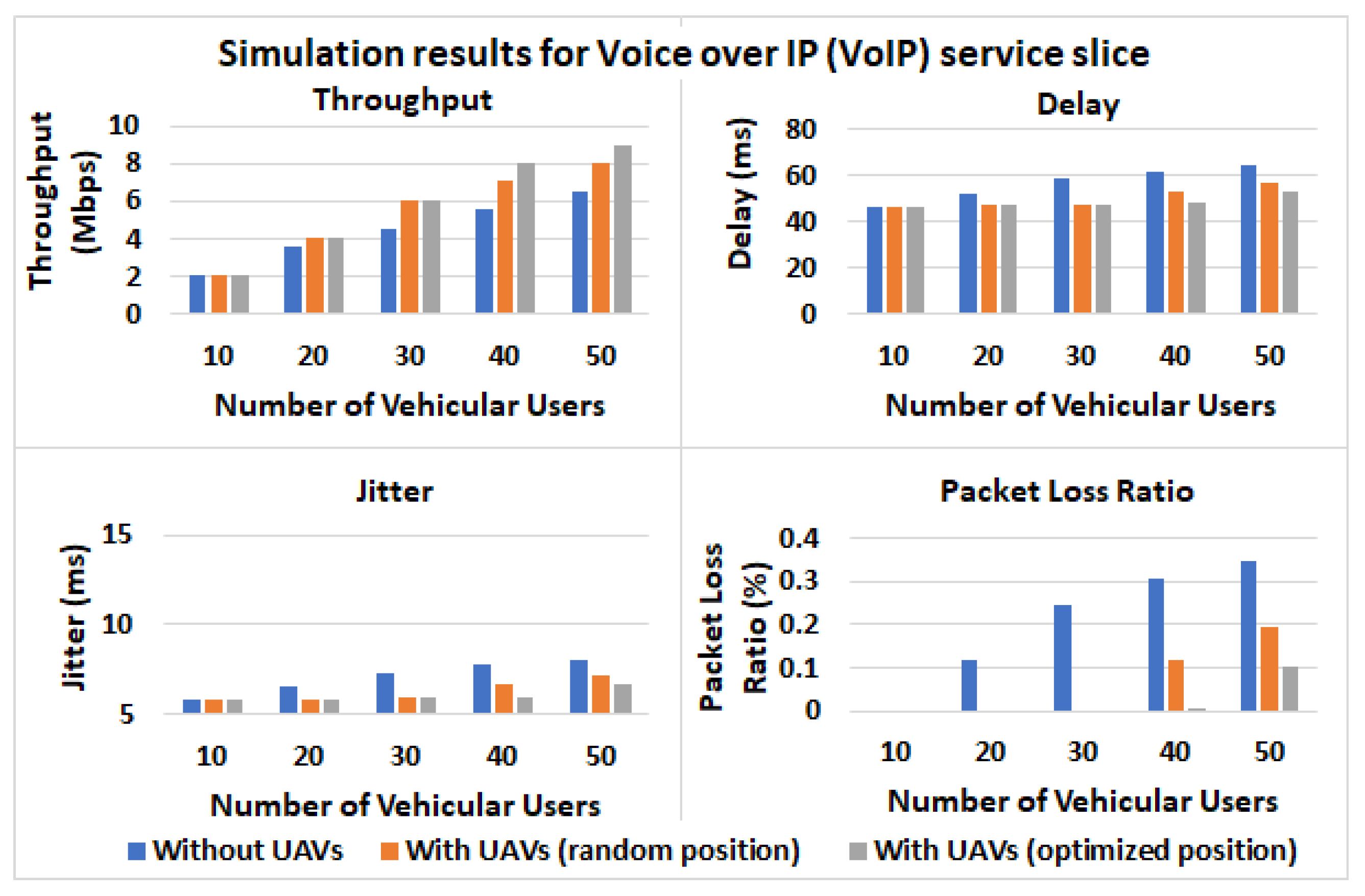
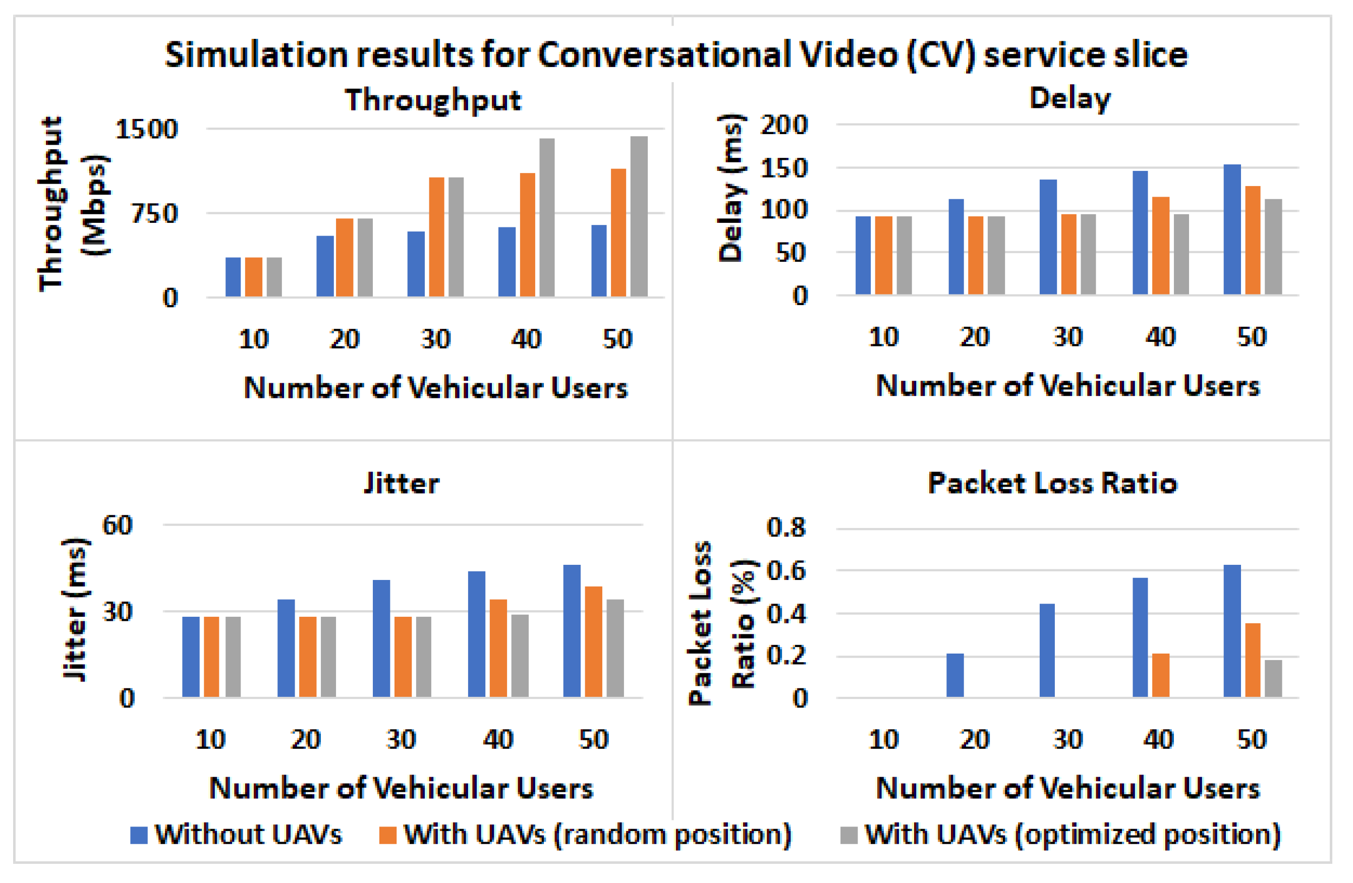
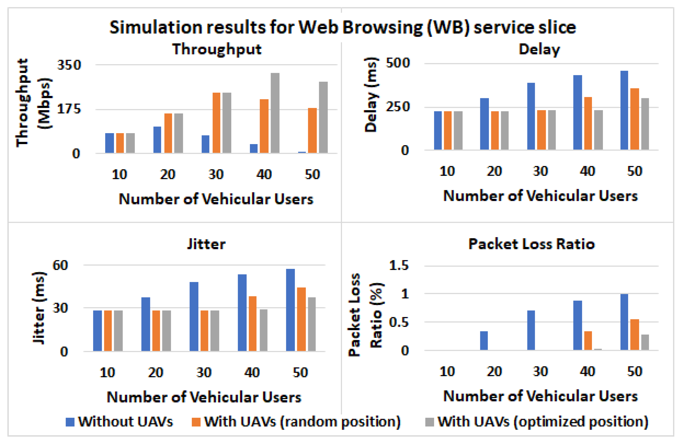
The parameters considered for the performance evaluation include the throughput, the end-to-end delay, the jitter and the packet loss ratio. As observed from the simulation results, where the positions of the ARNs are optimized, the proposed scheme succeeds improved performance since optimal channel conditions are provided to the vehicular users. In particular, as presented in Figure 5, for the ANav service slice, in the case where ARNs obtain optimized positions, the proposed scheme succeeds up to $2.01$ Mbps higher throughput than these succeeded when the ARNs obtain a random position, as well as up to $5.39$ Mbps higher throughput in comparison with the case where no ARNs used. At the same time, up to $0.6$ ms, $0.07$ ms and $17.9\%$ lower values are observed for both the packet transfer delay, the jitter and the packet loss ratio factors, respectively. Similarly, Figure 6, Figure 7 and Figure 8 present the corresponding results for the VoIP, the CV and the WB services, respectively. As it can be observed, in the case of the VoIP service slice, where the ARNs obtain optimized positions, up to $0.91$ Mbps and $2.45$ Mbps higher throughput is achieved, in comparison with the cases where either the ARNs obtain random positions or no ARNs used, respectively. At the same time, for the VoIP service slice, up to $11.27$ ms, $0.24$ ms and $24.5\%$ lower values are observed for the delay, the jitter and the packet loss ratio factors, respectively. In addition, similar results are observed in the case of the CV service slice, which is the most demanding service in terms of throughput in our simulation. In particular, in the case of the CV service slice up to $296.7$ Mbps and $793.2$ Mbps, higher throughput is observed where the positions of the ARNs are optimized, compared with the cases where the ARNs obtain random positions or no ARNs exist. In addition, similar to the other service slices, the values for the delay, the jitter and the packet loss ratio are up to $41.2$ ms, $12.35$ ms and $44\%$ lower than those observed in the other two cases, where either ARNs are not used or their geographical positions are not optimized. Finally, for the WB service slice, the proposed scheme succeeds up to $105.5$ Mbps and $282.1$ Mbps higher throughput from the other two cases, respectively, and up to $157.7$ ms, $19.71$ ms and $70.5\%$ lower values for the delay, the jitter and the packet loss ratio, respectively, where the ARNs obtain optimal geographical positions.

In some cases where the service requirements cannot be met from the RSUs, the use of ARNs results in critical improvements of the system performance and thus to the satisfaction of the constraints of the aforementioned services. Indicatively, in the case of the CV service, the maximum acceptable is equal to 150 ms. In this case, when the number of vehicular users becomes equal to 50, the observed packet transfer delay is equal to $154.29$ ms (Figure 7) and thus the delay constraint is not satisfied. However, with the use of ARNs, even when their position has not been optimized, the observed packet transfer delay is less than 150 ms and thus it can be considered a satisfied QoS parameter. Additionally, in the case of the WB service, when the number of vehicular users becomes equal to 50, the delay constraint of the 300 ms is satisfied only in the case where ARNs with optimized positions are used (Figure 8). In addition, similar improvements are observed in the case of the packet loss ratio factor. Specifically, considering the results for the entire services (Figure 5, Figure 6, Figure 7 and Figure 8), when no ARNs used the packet loss ratio constraint is satisfied only for the case of 10 users. On the contrary, when ARNs used the packet loss ratio is satisfied for up to 30 users, while in the case where the ARNs obtain optimal positions, the packet loss ratio factor is satisfied for up to 40 users.

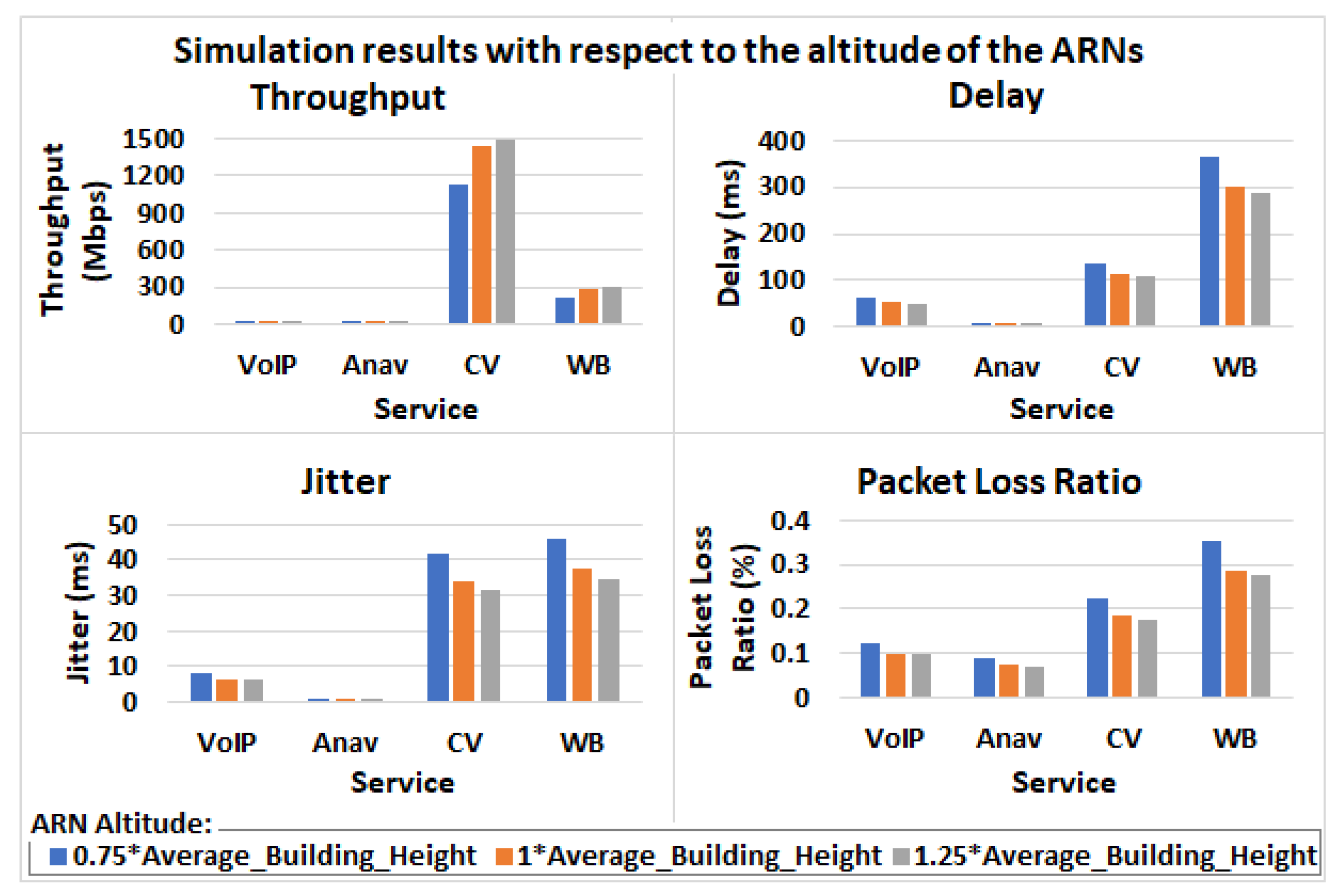
Furthermore, Figure 9 presents how the altitude of ARNs affects the performance of the system. As it can be observed, when the altitude of the ARNs is $25\%$ higher than the average height of the buildings, better performance is observed for the entire services in terms of throughput, delay, jitter and packet loss ratio. On the contrary, worse performance is observed when the ARNs obtain lower altitude than the average height of the building, since in this case, worse channel conditions occur due to the increased number of obstacles that exist between the ARNs and the vehicular users.

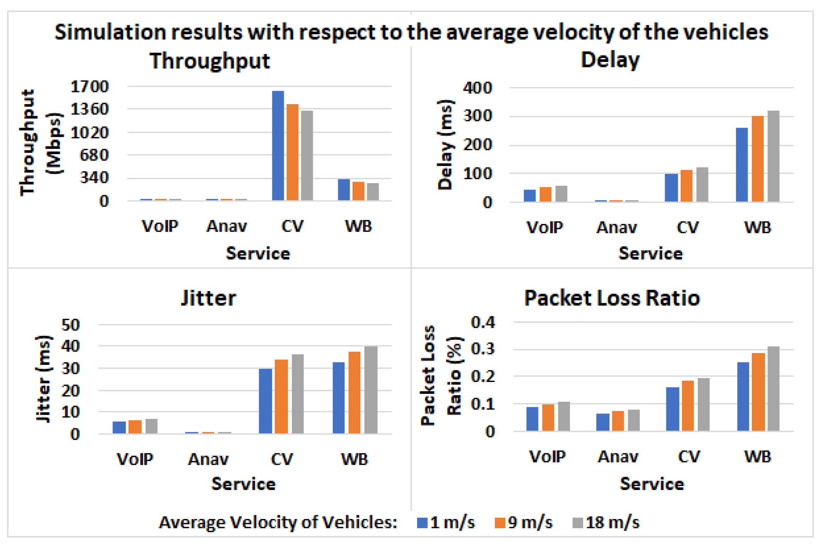
Accordingly, Figure 10 presents how the average velocity of the vehicles affects the performance of the system. In particular, as the vehicles move with lower velocity, the performance of the system is maximized since each ARN remains for a longer period of time at a specific position without requiring the execution of the IFT algorithm for selecting another optimal position. On the contrary, when the average velocity of the vehicles is increased, the overall performance of the system is reduced. However, as it is observed, if we compare the results presented in Figure 10 with the ones presented in Figure 6, Figure 7 and Figure 8, where the vehicles are supposed to have average velocity equal to 9 m/s, even when the vehicles obtain an average velocity equal to 18 m/s, the performance achieved from the proposed scheme is better than the one observed in the case where no ARNs used.

Regarding the simulation results, it is obvious that when the ARNs obtain optimal positions, even if the same amount of communication resources is committed by the algorithm, improved performance is achieved since improved channel conditions are established. As a conclusion of this situation, it can be said that from the network provider’s point of view, this means that communication resources can be released in cases where the requirements of the services are satisfied. On the other hand, from the user’s point of view, even better QoS can be perceived.

7. Conclusions

In this paper, a network slicing scheme for 5G networks was proposed, aimed at the optimization of the performance of vehicular services. In particular, the proposed network architecture consists of UAVs acting as ARNs and RSUs that provide communication resources to vehicular users. Moreover, the position of each ARN is optimized by applying the proposed IFT algorithm. Regarding the proposed scheme, each ARN maintains its own RBs, while each RSU maintains an LVRP which contains LRBs and SRBs. An SDN controller provides centralized control of the entire architecture, while at the same time, it maintains a VRP, where the SRBs of the RSUs are stored. The satisfaction grade of each user service is monitored considering both the QoS and the SINR factors. If the satisfaction grade is higher than the predefined threshold value, the service requirements can be satisfied from the remaining RBs of the RSU or ARN where the user is connected. On the contrary, if the estimated satisfaction grade is lower than the predefined threshold value, the RSU or ARN borrows extra RBs from the corresponding virtual resource pool. Performance evaluation shows that enhanced performance is achieved where the geographical positions of the ARNs are optimized, since in this case, improved channel conditions are provided to the users.

References

- Kazemifard, N.; Shah-Mansouri, V. Minimum delay function placement and resource allocation for Open RAN (O-RAN) 5G networks. Comput. Netw. 2021, 188, 107809. [Google Scholar] [CrossRef]
- TR 21.915 (V15.0.0): Digital Cellular Telecommunications System (Phase 2+) (GSM); LTE; 5G; (Rel.15); Technical Specification, 3GPP; Universal Mobile Telecommunications System (UMTS): Sophia Antipolis, France, 2019.
- Jiang, X.; Sheng, M.; Zhao, N.; Xing, C.; Lu, W.; Wang, X. Green UAV communications for 6G: A survey. Chin. J. Aeronaut. 2021. [Google Scholar] [CrossRef]
- Raj, A.S.A.; Palanichamy, Y. An aerial intelligent relay-road side unit (AIR-RSU) framework for modern intelligent transportation system. Peer-to-Peer Netw. Appl. 2020, 13, 965–986. [Google Scholar] [CrossRef]
- Lemeshko, O.; Yeremenko, O.; Kovalenko, T.; Al-Dulaimi, A.M.; Al-Dulaimi, M.K. Comparative Analysis of the Resource Blocks Allocation Balancing Model in the LTE Downlink Using RAT 1 with Existing Solutions. In Proceedings of the 2018 International Scientific-Practical Conference Problems of Infocommunications, Science and Technology (PIC S&T), Kharkiv, Ukraine, 9–12 October 2018; pp. 701–704. [Google Scholar]
- Raju, V.; Jayagopal, R. An Arithmetic Operations of Icosagonal fuzzy number using Alpha cut. Int. J. Pure Appl. Math. 2018, 120, 137–145. [Google Scholar]
- Next Generation Mobile Network Alliance (NGMN). 2021. Available online: https://www.ngmn.org/ (accessed on 20 June 2021).
- Marinova, S.; Lin, T.; Bannazadeh, H.; Leon-Garcia, A. End-to-end network slicing for future wireless in multi-region cloud platforms. Comput. Netw. 2020, 177, 107298. [Google Scholar] [CrossRef]
- Nojima, D.; Katsumata, Y.; Shimojo, T.; Morihiro, Y.; Asai, T.; Yamada, A.; Iwashina, S. Resource isolation in RAN part while utilizing ordinary scheduling algorithm for network slicing. In Proceedings of the 2018 IEEE 87th Vehicular Technology Conference (VTC Spring), Porto, Portugal, 3–6 June 2018; pp. 1–5. [Google Scholar]
- Joung, J. Random space–time line code with proportional fairness scheduling. IEEE Access 2020, 8, 35253–35262. [Google Scholar] [CrossRef]
- Ge, X. Ultra-reliable low-latency communications in autonomous vehicular networks. IEEE Trans. Veh. Technol. 2019, 68, 5005–5016. [Google Scholar] [CrossRef] [Green Version]
- Piro, G.; Grieco, L.A.; Boggia, G.; Fortuna, R.; Camarda, P. Two-level downlink scheduling for real-time multimedia services in LTE networks. IEEE Trans. Multimed. 2011, 13, 1052–1065. [Google Scholar] [CrossRef]
- Ouaissa, M.; Rhattoy, A.; Lahmer, M. Comparative performance study of QoS downlink scheduling algorithms in LTE system for M2M communications. In Proceedings of the International Conference Europe Middle East & North Africa Information Systems and Technologies to Support Learning, Fez, Morocco, 25–27 October 2018; Springer: Berlin/Heidelberg, Germany, 2018; pp. 216–224. [Google Scholar]
- Skondras, E.; Michalas, A.; Sgora, A.; Vergados, D.D. A downlink scheduler supporting real time services in LTE cellular networks. In Proceedings of the 2015 6th International Conference on Information, Intelligence, Systems and Applications (IISA), Corfu, Greece, 6–8 July 2015; pp. 1–6. [Google Scholar]
- Skondras, E.; Michalas, A.; Sgora, A.; Vergados, D.D. QoS-aware scheduling in LTE-A networks with SDN control. In Proceedings of the 2016 7th International Conference on Information, Intelligence, Systems & Applications (IISA), Chalkidiki, Greece, 13–15 July 2016; pp. 1–6. [Google Scholar]
- Mihovska, A.; Prasad, R. Overview of 5G New Radio and Carrier Aggregation: 5G and Beyond Networks. In Proceedings of the 2020 23rd International Symposium on Wireless Personal Multimedia Communications (WPMC), Okayama, Japan, 18–26 October 2020; pp. 1–6. [Google Scholar]
- Haci, H.; Abdelbari, A. Throughput enhanced scheduling (TES) scheme for ultra-dense networks. Int. J. Commun. Syst. 2020, 33, e4229. [Google Scholar] [CrossRef]
- Shi, W.; Zhou, H.; Li, J.; Xu, W.; Zhang, N.; Shen, X. Drone assisted vehicular networks: Architecture, challenges and opportunities. IEEE Netw. 2018, 32, 130–137. [Google Scholar] [CrossRef]
- Michailidis, E.T.; Potirakis, S.M.; Kanatas, A.G. AI-Inspired Non-Terrestrial Networks for IIoT: Review on Enabling Technologies and Applications. IoT 2020, 1, 21–48. [Google Scholar] [CrossRef]
- Khabbaz, M.; Antoun, J.; Assi, C. Modeling and performance analysis of UAV-assisted vehicular networks. IEEE Trans. Veh. Technol. 2019, 68, 8384–8396. [Google Scholar] [CrossRef]
- Fawaz, W. Effect of non-cooperative vehicles on path connectivity in vehicular networks: A theoretical analysis and UAV-based remedy. Veh. Commun. 2018, 11, 12–19. [Google Scholar] [CrossRef]
- Zhou, Y.; Cheng, N.; Lu, N.; Shen, X.S. Multi-UAV-aided networks: Aerial-ground cooperative vehicular networking architecture. IEEE Veh. Technol. Mag. 2015, 10, 36–44. [Google Scholar] [CrossRef]
- Hong, K.; Lillethun, D.; Ramachandran, U.; Ottenwälder, B.; Koldehofe, B. Mobile fog: A programming model for large-scale applications on the internet of things. In Proceedings of the Second ACM SIGCOMM Workshop on Mobile Cloud Computing, Hong Kong, China, 16 August 2013; pp. 15–20. [Google Scholar]
- Bithas, P.S.; Michailidis, E.T.; Nomikos, N.; Vouyioukas, D.; Kanatas, A.G. A survey on machine-learning techniques for UAV-based communications. Sensors 2019, 19, 5170. [Google Scholar] [CrossRef] [PubMed] [Green Version]
- Secinti, G.; Darian, P.B.; Canberk, B.; Chowdhury, K.R. SDNs in the sky: Robust end-to-end connectivity for aerial vehicular networks. IEEE Commun. Mag. 2018, 56, 16–21. [Google Scholar] [CrossRef]
- Nomikos, N.; Michailidis, E.T.; Trakadas, P.; Vouyioukas, D.; Karl, H.; Martrat, J.; Zahariadis, T.; Papadopoulos, K.; Voliotis, S. A UAV-based moving 5G RAN for massive connectivity of mobile users and IoT devices. Veh. Commun. 2020, 25, 100250. [Google Scholar] [CrossRef]
- Michailidis, E.T.; Miridakis, N.I.; Michalas, A.; Skondras, E.; Vergados, D.J. Energy Optimization in Dual-RIS UAV-Aided MEC-Enabled Internet of Vehicles. Sensors 2021, 21, 4392. [Google Scholar] [CrossRef]
- Cheng, N.; Xu, W.; Shi, W.; Zhou, Y.; Lu, N.; Zhou, H.; Shen, X. Air-ground integrated mobile edge networks: Architecture, challenges, and opportunities. IEEE Commun. Mag. 2018, 56, 26–32. [Google Scholar] [CrossRef] [Green Version]
- Faraci, G.; Grasso, C.; Schembra, G. Design of a 5G network slice extension with MEC UAVs managed with reinforcement learning. IEEE J. Sel. Areas Commun. 2020, 38, 2356–2371. [Google Scholar] [CrossRef]
- Yuan, Z.; Muntean, G.M. AirSlice: A Network Slicing Framework for UAV Communications. IEEE Commun. Mag. 2020, 58, 62–68. [Google Scholar] [CrossRef]
- Xilouris, G.K.; Batistatos, M.C.; Athanasiadou, G.E.; Tsoulos, G.; Pervaiz, H.B.; Zarakovitis, C.C. UAV-assisted 5G network architecture with slicing and virtualization. In Proceedings of the 2018 IEEE Globecom Workshops (GC Wkshps), Abu Dhabi, United Arab Emirates, 9–13 December 2018; pp. 1–7. [Google Scholar]
- Garcia, A.E.; Hofmann, S.; Sous, C.; Garcia, L.; Baltaci, A.; Bach, C.; Wellens, R.; Gera, D.; Schupke, D.; Gonzalez, H.E. Performance evaluation of network slicing for aerial vehicle communications. In Proceedings of the 2019 IEEE International Conference on Communications Workshops (ICC Workshops), Shanghai, China, 22–24 May 2019; pp. 1–6. [Google Scholar]
- Zhang, S.; Quan, W.; Li, J.; Shi, W.; Yang, P.; Shen, X. Air-ground integrated vehicular network slicing with content pushing and caching. IEEE J. Sel. Areas Commun. 2018, 36, 2114–2127. [Google Scholar] [CrossRef] [Green Version]
- Lyu, F.; Yang, P.; Wu, H.; Zhou, C.; Ren, J.; Zhang, Y.; Shen, X. Service-Oriented Dynamic Resource Slicing and Optimization for Space-Air-Ground Integrated Vehicular Networks. IEEE Trans. Intell. Transp. Syst. 2021. [Google Scholar] [CrossRef]
- Grasso, C.; Schembra, G. A fleet of MEC UAVs to extend a 5G network slice for video monitoring with low-latency constraints. J. Sens. Actuator Netw. 2019, 8, 3. [Google Scholar] [CrossRef] [Green Version]
- Skondras, E.; Michalas, A.; Vergados, D.J.; Michailidis, E.T.; Miridakis, N.I.; Vergados, D.D. Network Slicing on 5G Vehicular Cloud Computing Systems. Electronics 2021, 10, 1474. [Google Scholar] [CrossRef]
- Zadeh, L.A. Fuzzy logic. Computer 1988, 21, 83–93. [Google Scholar] [CrossRef]
- Singh, H.; Gupta, M.M.; Meitzler, T.; Hou, Z.G.; Garg, K.K.; Solo, A.M.; Zadeh, L.A. Real-life applications of fuzzy logic. Adv. Fuzzy Syst. 2013. [Google Scholar] [CrossRef]
- View on 5G Architecture (Version 3); 5G PPP Architecture Working Group: Heidelberg, Germany, 2019.
- Skondras, E.; Michalas, A.; Vergados, D.D. Mobility management on 5g vehicular cloud computing systems. Veh. Commun. 2019, 16, 15–44. [Google Scholar] [CrossRef]
- Desogus, C.; Anedda, M.; Murroni, M. Real-time load optimization for multimedia delivery content over heterogeneuos wireless network using a MEW approach. In Proceedings of the 2017 IEEE International Symposium on Broadband Multimedia Systems and Broadcasting (BMSB), Cagliari, Italy, 7–9 June 2017; pp. 1–4. [Google Scholar]
- Skondras, E.; Michalas, A.; Vergados, D.J.; Michailidis, E.T.; Miridakis, N.I. A Network Slicing Algorithm for 5G Vehicular Networks. In Proceedings of the 2021 12th International Conference on Information, Intelligence, Systems and Applications (IISA), Crete, Greece, 12–14 July 2021; pp. 1–6. [Google Scholar]
- Skondras, E.; Sgora, A.; Michalas, A.; Vergados, D.D. An analytic network process and trapezoidal interval-valued fuzzy technique for order preference by similarity to ideal solution network access selection method. Int. J. Commun. Syst. 2016, 29, 307–329. [Google Scholar] [CrossRef]
- Charilas, D.E.; Markaki, O.I.; Psarras, J.; Constantinou, P. Application of fuzzy AHP and ELECTRE to network selection. In Mobile Lightweight Wireless Systems; Springer: Berlin/Heidelberg, Germany, 2009; pp. 63–73. [Google Scholar]
- Goyal, R.K.; Kaushal, S.; Sangaiah, A.K. The utility based non-linear fuzzy AHP optimization model for network selection in heterogeneous wireless networks. Appl. Soft Comput. 2017, 67, 800–811. [Google Scholar] [CrossRef]
- Skondras, E.; Michalas, A.; Tsolis, N.; Vergados, D.D. A network selection scheme with adaptive criteria weights for 5g vehicular systems. In Proceedings of the 2018 9th International Conference on Information, Intelligence, Systems and Applications (IISA), Zakynthos, Greece, 23–25 July 2018; pp. 1–7. [Google Scholar]
- Skondras, E.; Michalas, A.; Tsolis, N.; Vergados, D.D. A VHO scheme for supporting healthcare services in 5G vehicular cloud computing systems. In Proceedings of the 2018 Wireless Telecommunications Symposium (WTS), Phoenix, AZ, USA, 17–20 April 2018; pp. 1–6. [Google Scholar]
- Skondras, E.; Siountri, K.; Michalas, A.; Vergados, D.D. A route selection scheme for supporting virtual tours in sites with cultural interest using drones. In Proceedings of the 2018 9th International Conference on Information, Intelligence, Systems and Applications (IISA), Zakynthos, Greece, 23–25 July 2018; pp. 1–6. [Google Scholar]
- Hwang, C.L.; Yoon, K. Multiple Attribute Decision Making; Springer: Berlin/Heidelberg, Germany, 1981. [Google Scholar]
- Ncibi, K.; Hadji, R.; Hamdi, M.; Mokadem, N.; Abbes, M.; Khelifi, F.; Zighmi, K.; Hamed, Y. Application of the analytic hierarchy process to weight the criteria used to determine the Water Quality Index of groundwater in the northeastern basin of the Sidi Bouzid region, Central Tunisia. Euro-Mediterr. J. Environ. Integr. 2020, 5, 1–15. [Google Scholar] [CrossRef]
- Elshaboury, N.; Attia, T.; Marzouk, M. Comparison of several aggregation techniques for deriving analytic network process weights. Water Resour. Manag. 2020, 34, 4901–4919. [Google Scholar] [CrossRef]
- Ashtiani, B.; Haghighirad, F.; Makui, A. Extension of fuzzy TOPSIS method based on interval-valued fuzzy sets. Appl. Soft Comput. 2009, 9, 457–461. [Google Scholar] [CrossRef]
- Open Street Map (OSM). Available online: https://www.openstreetmap.org (accessed on 20 June 2021).
- Behrisch, M.; Bieker, L.; Erdmann, J.; Krajzewicz, D. SUMO–simulation of urban mobility: An overview. In Proceedings of the SIMUL 2011, The Third International Conference on Advances in System Simulation, Barcelona, Spain, 23–29 October 2011. [Google Scholar]
- Network Simulator 3 (NS3). Available online: https://www.nsnam.org/ (accessed on 20 June 2021).
- NS3 LTE-V2X Extension Module. Available online: https://github.com/eisbaer/v2x-lte (accessed on 20 June 2021).
- TR 36.814 (V9.0.0): Further advancements for E-UTRA physical layer aspects (Release 9). In Technical Specification Group Radio Access Network, 3GPP; Universal Mobile Telecommunications System (UMTS): Sophia Antipolis, France, 2010.
- TR 36.942 (V10.2.0): Radio Frequency (RF) system scenarios (Release 10). In Technical Specification Group Radio Access Network, 3GPP; Universal Mobile Telecommunications System (UMTS): Sophia Antipolis, France, 2011.
- NS3 OnOffApplication Class Reference. Available online: https://www.nsnam.org/doxygen/classns3_1_1_on_off_application.html (accessed on 20 June 2021).
- iLab Video Gene Big Data Team. Video Big Data: The Top 10 Most Demanding Videos on the Net. In Video Big Data Report; iLab Video Gene Big Data Team: Shenzhen, China, 2017. [Google Scholar]
- NS3 UdpTraceClient Class Reference. 2021. Available online: https://www.nsnam.org/doxygen/structns3_1_1_udp_trace_client.html (accessed on 20 June 2021).
- 3GPP HTTP applications, NS3. 2021. Available online: https://www.nsnam.org/docs/models/html/applications.html (accessed on 20 June 2021).
Figure 1.
The layer stack of the proposed scheme.
Figure 2.
The S values range as obtained using the Mamdani fuzzy Inference System.
Figure 3.
The proposed network slicing architecture.
Figure 4.
The simulated topology.
Figure 5.
The simulation results for the autonomous navigation (ANav) service slice.
Figure 6.
The simulation results for the voice over IP (VoIP) service slice.
Figure 7.
The simulation results for the conversational video (CV) service slice.
Figure 8.
The simulation results for the Web browsing (WB) service slice.
Figure 9.
The simulation results with respect to the altitude of the ARNs.
Figure 10.
The simulation results with respect to the average velocity of the vehicles.