Article

Biomass Estimation of Agave durangensis Gentry Using High-Resolution Images in Nombre de Dios, Durango

by
Pablito Marcelo López-Serrano
1,
Gerardo A. Núñez-Fernández
2,
Rolando Alvarado-Barrera
3,
Emily García-Montiel
4,
Hugo Ramírez-Aldaba
4,* and
Melissa Bocanegra-Salazar
4
1
Instituto de Silvicultura e Industria de la Madera, Universidad Juárez del Estado de Durango, Durango 34000, Durango, Mexico
2
Geomática Forestal y Medio Ambiente S.C., Durango 34000, Durango, Mexico
3
Instituto Tecnológico Superior de Santiago Papasquiaro, Santiago Papasquiaro 34630, Durango, Mexico
4
Facultad de Ciencias Forestales y Ambientales, Universidad Juárez del Estado de Durango, Durango 34000, Durango, Mexico
*
Author to whom correspondence should be addressed.
Submission received: 11 May 2022 / Revised: 10 June 2022 / Accepted: 11 June 2022 / Published: 15 June 2022

Abstract

:
The high demand for distilled agave products reduces wild populations. The use of geospatial technologies such as unmanned aerial vehicles (UAVs) offer enormous benefits in spatial and temporal resolution and lower costs than traditional direct field observation techniques for natural resource monitoring. The objective was to estimate the green biomass (Wt) of Agave durangensis Gentry using high-resolution images obtained by a UAV in Nombre de Dios, Durango. Random sampling was performed in the agave area. A Pearson correlation analysis was performed, followed by a regression analysis. The results showed that NDVI was the most correlated (r = 0.65). The regression analysis showed that the model obtained explains 59% (RMSE = 32.06 kg) of the total variability in the estimation of green biomass (Wt) of agave using images derived from the UAV. The best estimate was achieved with B1, B2, NDVI, GNDVI, EVI2, and SAVI as predictor variables. High-resolution images were shown to be a tool for estimating Wt of Agave durangensis Gentry.

Graphical Abstract

1. Introduction

Agaves belong to the Asparagaceae family and are one of the most important groups of plants from a cultural and economic point of view. The center of greatest richness and concentration of the Asparagaceae family is Mexico where 251 species are distributed (76% of the total), with 177 endemic (70%) [1,2]. According to García-Mendoza [2], the most diverse and broadest genus of the family is agave with 210 species, of which 159 are found in Mexico, with 119 endemic species [1,2].
Agave has been used for thousands of years, due to its numerous benefits, e.g., the distilled beverages known generically as mezcals [3]. The first records of mezcal production date back to the early 16th century in the western part of the country, extending to regions that today comprise the states of San Luis Potosí, Zacatecas, and Durango [4]. Its production is the most important agro-industrial activity and is carried out in at least 20 states of the Mexican Republic, taking advantage of wild and cultivated populations [3]. Mezcal is officially regulated by Mexican Standard NOM-070-SCFI-2016 and the states with denomination of origin are Durango, Zacatecas, Michoacán, Puebla, Guerrero, Tamaulipas, San Luis Potosí, Guanajuato, and Oaxaca [5]. Mezcal production at the national level has increased in the last 5 years, going from being a low-cost drink and considered for the exclusive consumption of low-income people to being positioned almost on a par with tequila, gaining great renown at the national level and beginning to be placed on the international market with great acceptance [6]. Currently, in the state of Durango, there are only three certified factories and 10 mezcal bottling plants distributed mainly in the municipalities of Nombre de Dios, Mezquital, and Durango [4,7]. In this context, mezcal production has been the main cause of the decline in wild populations of the Agave genus, since its intensive exploitation puts the species at risk and could even lead to extinction [8,9]. Therefore, it represents a challenge to generate methodologies that allow sustainable management in such a way that the relevant ecological, economic, and social functions, at local, national, and global scales, of this type of ecosystem are fulfilled [3].
The development of technology has allowed the acquisition of satellite images at different resolutions through different remote sensors for the evaluation of ecological aspects of vegetation at a large scale, providing valuable information for the sustainable management of natural resources [10,11]. In specific cases, they are used for crop mapping and assessment of agave leaf biomass [12,13,14]. However, a common problem found with the use of this type of technologies is the cost and the availability of high-resolution images for the evaluation of natural resources [15].
In this sense, recent advances in aerial photogrammetry and remote sensing techniques contribute to solving environmental problems [16,17,18,19]. Specifically, with the emergence of unmanned aerial vehicles (UAVs), these techniques offer enormous benefits in spatial and temporal resolution and low costs relative to traditional direct field observation techniques [20,21,22]. UAVs provide aerial photographs and spectral information of terrestrial ecosystems in real time with high precision, thanks to the ability to use different multispectral sensors and the integration of a global positioning system (GPS) in its structure [23,24]. There are a range of sensors used for vegetation analysis; these sensors have different spectral resolutions, such as cameras with red, green, and blue (RGB) channels, as well as multispectral, hyperspectral, and thermal sensors [25]. In this context, UAVs allow transporting these sensors in order to collect information with higher spatiotemporal resolution for monitoring the growth and development of different crops in precision agriculture [15,26]. Generally, this monitoring is carried out through the generation of vegetation indices (VIs), which are algebraic combinations of the spectral bands integrated in each sensor (multispectral), in order to highlight the vigor of the vegetation and its reflectance properties [27].
Its multispectral composition allows differentiating the presence of vegetation on the land surface, separating it from other objects that are not of interest such as soil or urban areas [28,29,30,31,32]. Some studies have shown that VIs show high correlations with respect to biomass or volume production estimated from direct field measurement; hence, it has become common not only to use them to describe vegetation health but also to include them in the prediction of such variables [33,34,35]. In this context, the objective of this study was to estimate the green biomass of Agave durangensis Gentry using high-resolution images obtained by a UAV in an agave area in Nombre de Dios, Durango.

2. Materials and Methods
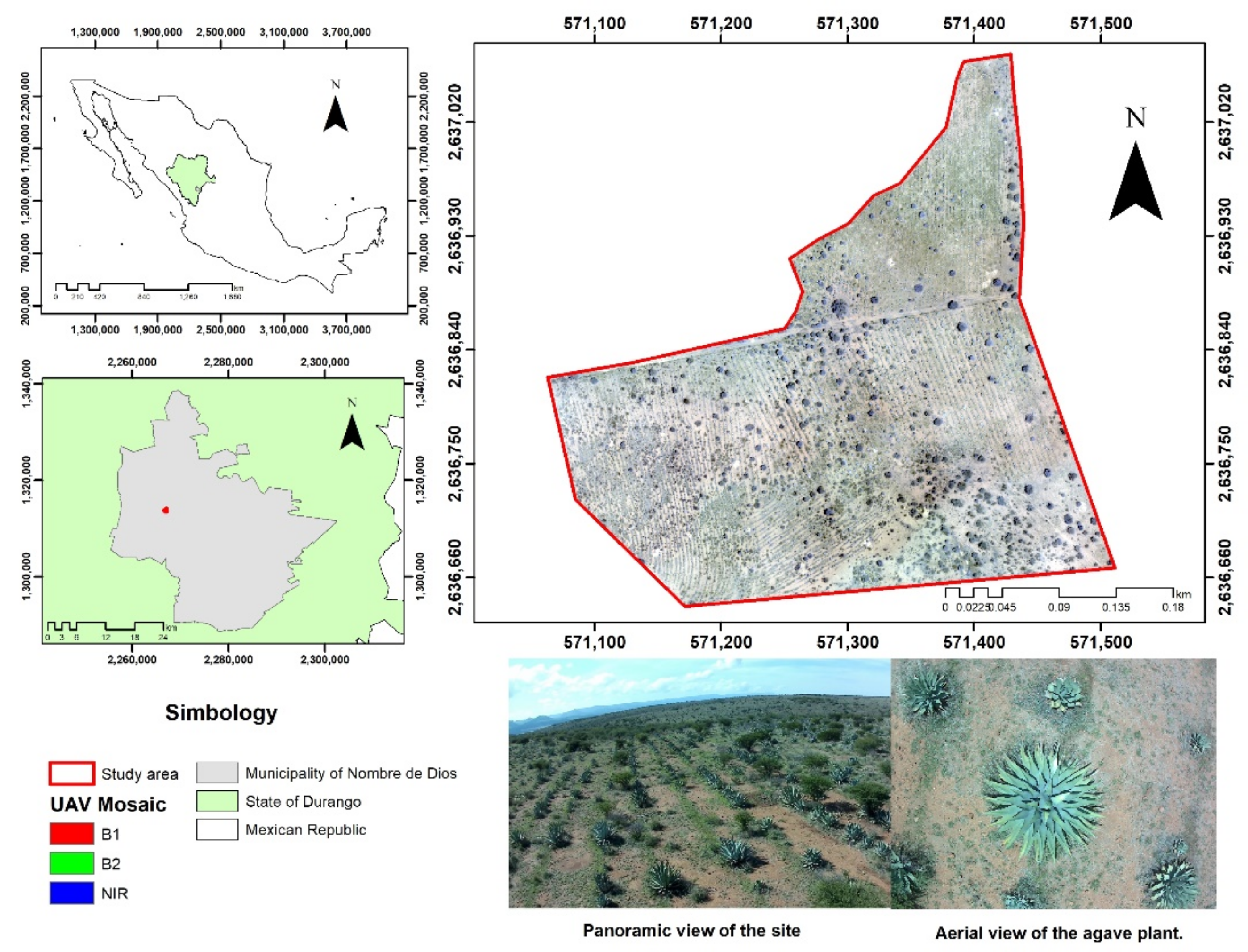
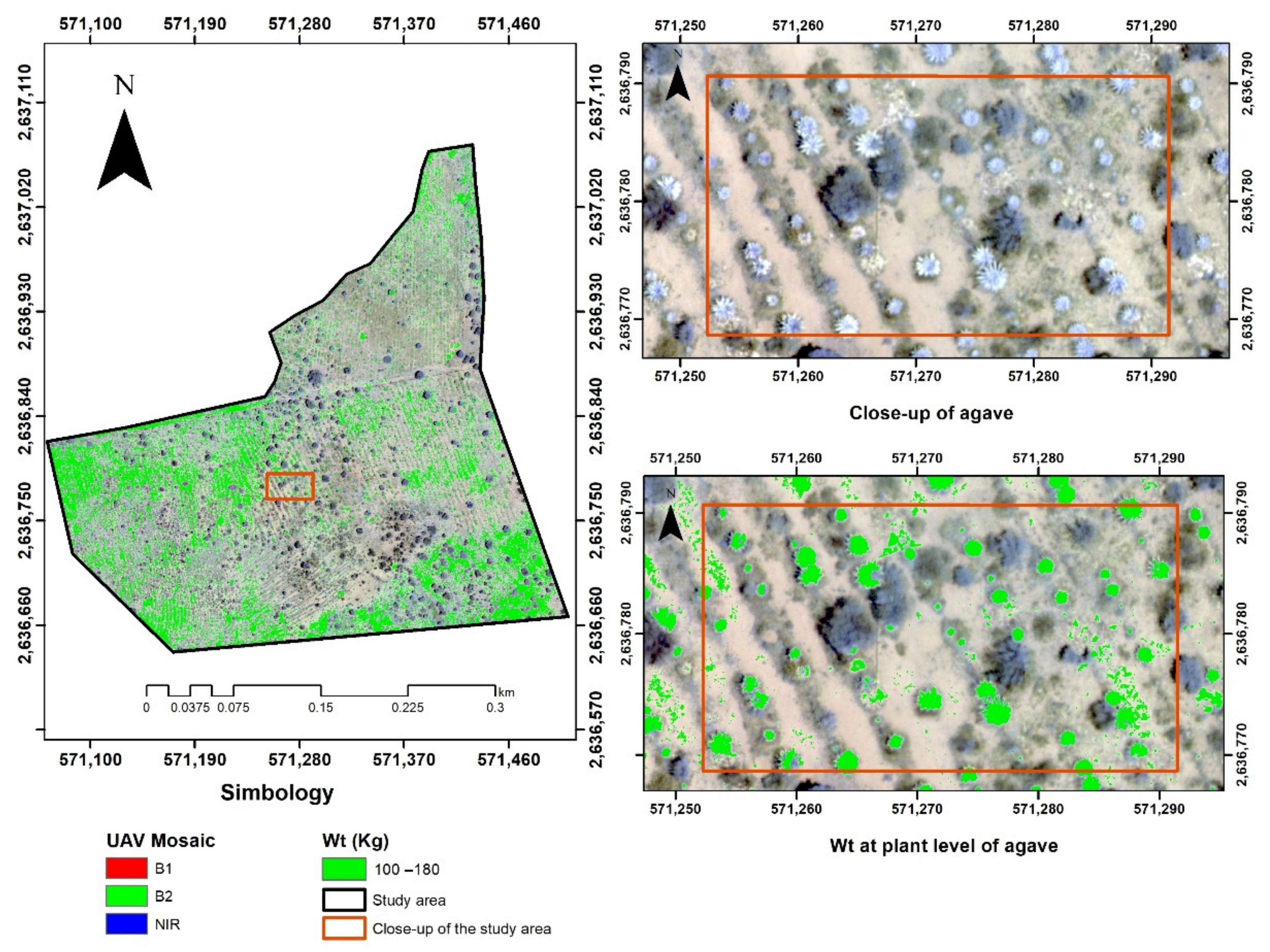
2.1. Study Area

The study area was located in the municipality of Nombre de Dios, in the State of Durango, in an area with the presence of agave of the species Agave durangensis Gentry, with an area of 15 ha (Figure 1). The area has a 5% slope. The climate in the area is semiarid (BS) with rainfall in summer. The average rainfall is 520 mm, and the average annual temperature is 29 °C. The predominant soil type is Regosol.

2.2. Estimation of Biomass

For the calculation of green biomass in the field, 40 agave plants were randomly sampled in the area. In each agave plant, direct measurements were made of the diameter of cover (D), considered as the average aerial cover of the plant measured from north to south and from east to west. On the other hand, the total height (At) of each agave was measured, considered as the vertical distance from the ground to the highest aerial part of the plant. Both measurements were made using a flexometer. In addition, the location of the plant was recorded using a Trimble geo 7x Global Navigation Satellite System (GNSS) handheld data collector, which guaranteed maximum precision in the location of each plant sampled.
On the basis of the information obtained from the field inventory of agaves, the total individual green biomass (Wt) was calculated using the allometric equation for the species Agave durangensis Gentry in the state of Durango (Table 1), obtained from the forest planning system for arid zones (SiFoZa-http://fcfposgrado.ujed.mx/sifoza, accessed on 10 June 2022).

2.3. Information Obtained by the Unmanned Aerial Vehicle (UAV)

An eBee UAV was used to obtain high-resolution images. This drone is designed to collect data efficiently and safely, in order to map and monitor crops quickly and easily. It is a fixed-wing drone, powered by an intelligent LiPo (lithium polymer) battery with a capacity of 3830 mAh and autonomy of 35 min of flight time. It has a wingspan of 96 cm, a weight of 700 g, and a maximum cruising speed of 65 km/h (40 mph). The eBee can cover up to 12 km2 and acquires images with a ground sampling distance (GSD) of up to 1.5 cm per pixel. A CANON S110NIR camera was mounted on the eBee UAV; this camera acquires images with 8 bit radiometric resolution in three channels of the electromagnetic sector (Table 2). The acquisition of the images is performed automatically during the flight controlled by the eBee’s intelligent pilot.

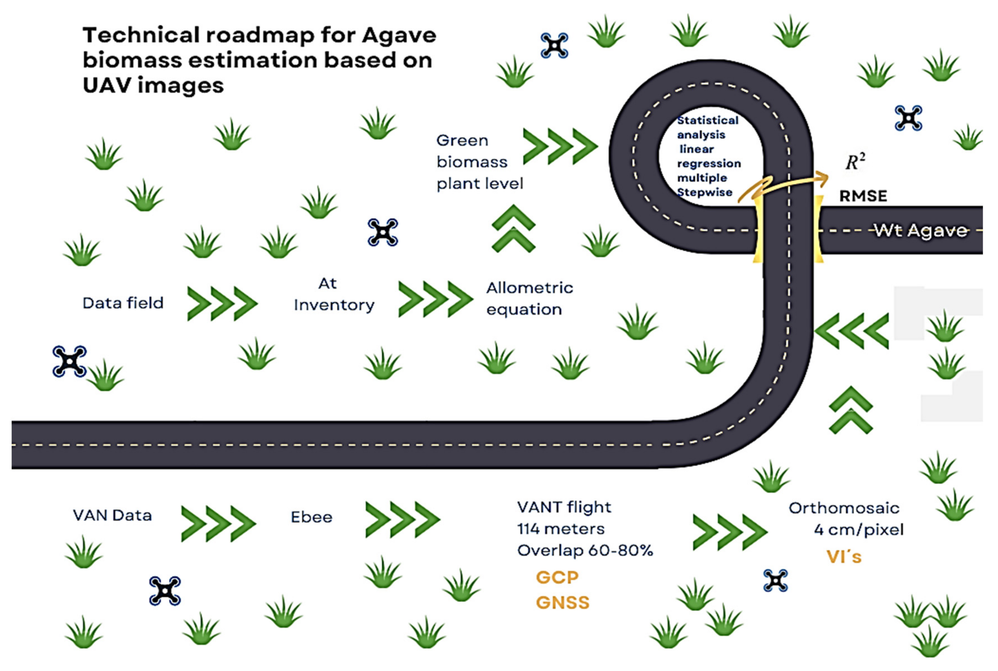
2.4. Acquisition and Processing of UAV Images

High-resolution images were acquired at a flight altitude of 114 m; flight time was 14 min for an area of 17.2 ha. A lateral overlap of 60% and a longitudinal overlap of 80% were used. The flight took place on a sunny and clear day, with a wind speed of 5 m/s. Five ground control points (GCPs) distributed over the flight area were established to improve the overall accuracy of the images. The GCPs were taken with coordinates in the Universal Transverse Mercator (UTM) system. For this purpose, two boards 1.5 m long by 20 cm wide were placed in the shape of a cross and were painted with a high-contrast color, for their facile recognition in the images of areas taken by the UAV. These GCPs were distributed in the flight area; one was placed in the center and the rest were distributed within the polygon of the study area. The GCP coordinate was taken by placing the GNSS in the center where the cross of the mark was formed. Later, in the Pix4D software, the coordinates of the GCPs taken in the field were imported using the Manager Manual Tie Points (MTP) function; using this process, the coordinates were linked to the images to improve the accuracy of the general geolocation of the orthomosaic. The images obtained by the UAV were processed to generate an orthomosaic with a uniform color; thus, it was not necessary to make any color balance adjustment of this orthomosaic with three bands with a resolution of 4 cm/pixel of the agave area. This process was performed in Pix4D software.
Once the orthomosaic was obtained, vegetation indices were generated with the objective of considering them as explicative spectral variables in the estimation of the green biomass of agave (Table 3). The selection of these indices in the present study was based on the spectral resolution of the sensor used (B1, B2, and NIR) and the application of the indices in other studies to evaluate the density of vegetation cover and separation of soil from vegetation [36,37,38,39,40].
Table 3. Vegetation indices used to estimate biomass.
IndexFormulaReference
NDVI (normalized difference vegetation index)(NIR − red)/(NIR + red)Rouse et al. [36]
GNDVI (green normalized difference vegetation index)(NIR − green)/(NIR + green)Gitelson et al. [37]
EVI2 (enhanced vegetation index)2.5 × (NIR − red)/((NIR + 2.4 × red) + 1)Jiang et al. [38]
SAVI (soil-adjusted vegetation index)((NIR − red))/((NIR + red + 0.16))Rondeaux et al. [39]
SR (simple ratio)NIR/redBirth and McVey [40]
The geolocations of each agave taken in the field, together with the estimated green biomass information, were superimposed with the orthomosaic generated from the UAV flight. With this, the mean of the pixel value was extracted with a circular buffer of 80 cm, in each of the spectral bands of the orthomosaic and the vegetation indices, using QGIS software [41].

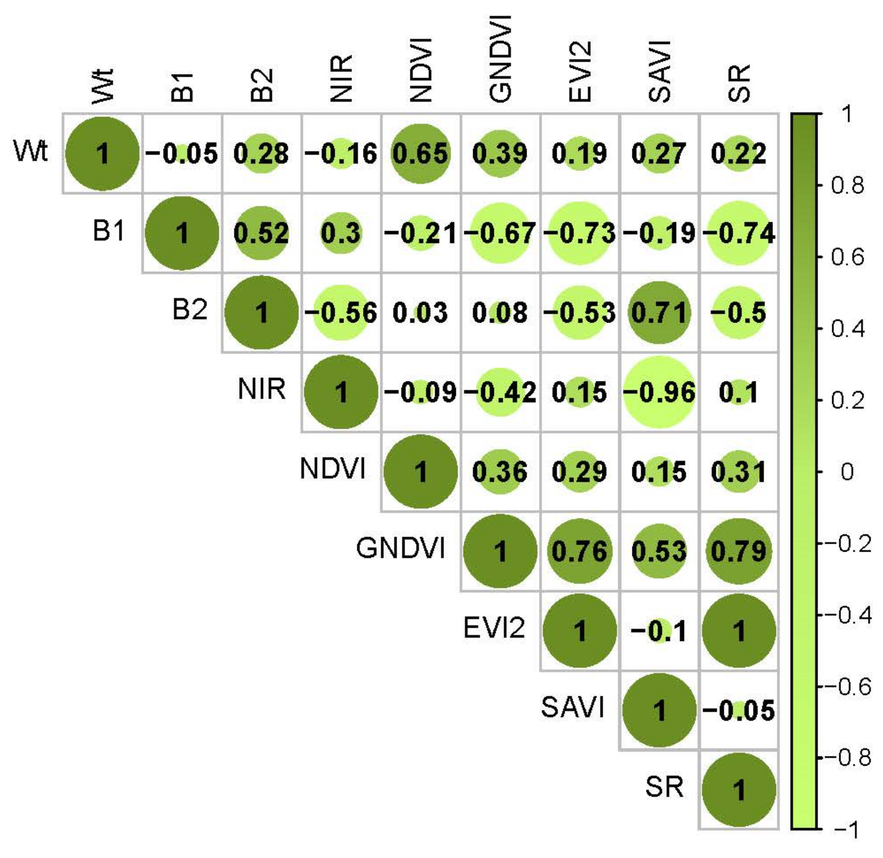
2.5. Statistical Analysis

In order to find the spectral variables that best estimate Wt, a correlation analysis was performed. Subsequently, multiple linear regression models were fitted to identify the variables that best predict Wt, using a stepwise procedure that used a combination of forward and backward selection. This procedure starts with no predictors, and then sequentially adds the most contributing predictors (such as forward selection). After adding each new variable, any variable that no longer provides an improvement in model fit is removed (similar to backward selection). Agave Wt was the dependent variable, while bands (B1, B2, and NIR) and vegetation indices (NDVI, GNDVI, EVI, SAVI, and DVI) were independent variables. This process was performed in R software [42], using the “MASS” library [43]. The model used was as follows:
y = β0 + β1 × 1 + β2 × 2 + … + βnXn + εi,
where y is the green biomass of agave, Xn denotes the spectral bands and vegetation index, βn denotes the regression coefficients, and εi is the random error.
In order to evaluate the model’s ability to fit, goodness-of-fit coefficients were calculated: coefficient of determination (R2) and root-mean-square error (RMSE).
R 2   =   1 i   =   1 n ( y i y ^ i ) 2 i   =   1 n ( y i y ¯ i ) 2 ,  
RMSE   =   i   =   1 n ( y i y ^ i ) 2 n p ,
where y i is the observed parameter,   y ^ i is the estimated parameter,   y ^ i is the mean of the parameter, n is the number of total observations, and p is the number of model parameters.
Once the best model was selected, the equation was applied to generate a distribution map of agave Wt in the study area; this process was performed using the library raster [44]. Figure 2 shows the technical roadmap used in this study for estimating agave biomass on the basis of UAV images.

3. Results

According to the inventory of agave plants in the plantation, it was found that the average D was 126.06 cm, while the average At was 101.53 cm and the average Wt was 71.81 kg (Table 4).
The correlations between Wt and the vegetation bands and indices are shown in Figure 3. The Pearson correlation coefficients (r) ranged from −0.02 to 0.65. The analysis showed a negative correlation with B1 and NIR, while B2, NDVI, GNDVI, GNDVI, EVI2, SAVI, and SR showed a positive linear association. NDVI was the spectral variable that showed the highest linear association with Wt (r = 0.65).
The regression analysis allowed generating a model involving spectral variables B1, B2, NDVI, GNDVI, GNDVI, EVI2, and SAVI derived from the high-resolution UAV images, which explained 59% (RMSE = 32.06 kg) of the total variability in the estimation of Wt of Agave durangensis Gentry (Table 5). Figure 4 illustrates the distribution of model residuals.
The model generated to estimate Wt was applied, and, as a result, a map was obtained showing the predicted values of Wt (Figure 5). Given the presence of tree, shrub, and grassland vegetation in the study area, only the Wt of the Agave durangensis Gentry vegetation is shown at the plant level. The predicted Wt ranged from 0 to 180 kg, with a mean of 57 kg. In the area, there was a variation of Wt in the spatial distribution of agave plants, given the different measures of cover (D) associated mainly with the most mature agave plants. (D ≥ 126 cm) in the study area.

4. Discussion

Remote sensing technologies, such as the one shown in this study, have been explored to make indirect estimates of important vegetation variables for their evaluation and monitoring in a more precise and low-cost manner. Obtaining high-resolution spectral information derived from a UAV allowed estimating the Wt of the species Agave durangensis Gentry in the present study. This is confirmed by Gitelson [29], who mentioned that the use of UAVs as novel tools allows a quantitative evaluation in a fast way and at a relatively low cost. In the present study, NDVI was the spectral variable that presented the highest correlation with agave Wt; this result is similar to that found in several studies that used UAVs to determine variables that facilitate the identification of tree species, shrubs, and agaves, as well as the nutritional status of crops such as sugarcane, wheat, and alfalfa [29,30,31,32], and the estimation of the fraction of vegetation cover [45,46]. As for the most contributing predictors in the most optimal model to estimate agave Wt, they were the spectral variables B1 and B2 and the vegetation indices of NDVI, GNDVI, EVI2, and SAVI. The contribution of these variables was related to the normalization of the index that provided a greater separation of green vegetation from background soil luminosity [36] and reduced the effects produced by topographic, atmospheric, and illumination factors [47]. In addition to the sensitivity of the green channel and red edge (B1, B2, and NIR) to the chlorophyll content at the leaf and canopy level of the vegetation, the indices increased with higher wavelengths, as observed by [33,34,35,48,49].
The sequentially fitted model for Wt estimation explained 59% of the total variance (R2 = 0.59; RMSE = 32.06 kg), with this value being below those obtained in different studies that used multispectral data for crop biomass assessment. For example, Rouse et al. [36] achieved an R2 of 0.86 for winter crops using a portable multispectral spectrometer, while Gitelson et al. [37] used data from an HJ1 satellite for biomass assessment in a wheat crop (R2 = 0.79). On the other hand, the result in the present study was similar to that obtained by Jiang et al. [38], who achieved an R2 of 0.58 for the evaluation of grassland biomass with images from the Sentinel-2 satellite platform with a spatial resolution of 10 m. For the case of agave crops, Rondeaux et al. [39] performed an estimation of agave (Agave sisalana) biomass using a generalized additive model analysis (explained deviation of 76% and RMSE of 5.15 Mg·ha−1) with Sentinel sensor images. Their results showed higher adjustment values than those found in the present study. It is worth mentioning that few studies have been found where the use of UAVs was applied for biomass estimation in agave. On the other hand, these values may have been lower because the estimation of biomass using spectral values, from any remote sensor, in crops where the density and vegetation cover are homogeneous (wheat, corn, and agave plantations) diminishes the effect of factors such as soil, soil moisture, and weeds. In this case, planting density in agave areas is heterogeneous, with the presence of weeds and the high presence of bare soil, affecting the establishment of a sensitive relationship between biomass and sensor spectral values. However, future studies can be applied to biomass estimation in arid and semiarid ecosystems using multispectral remote sensing on UAVs.

5. Conclusions

In this study, spectral variables derived from a UAV were tested to estimate biomass in an area of Agave durangensis Gentry. The variables B1, B2, NDVI, GNDVI, EVI2, and SAVI presented the best fit in the multiple linear regression model used for the estimation of agave biomass (R2 = 0.59; RMSE = 32.06 kg). This study demonstrates the use of UAVs for obtaining biomass information in natural agave areas, which allows its estimation in order to offer an alternative to remotely evaluate and monitor agave biomass. Lastly, it is recommended to evaluate this methodology in an agave plantation area (homogeneous crop) in order to assess its accuracy considering the effect of soil with vegetation using UAV-derived images.

Author Contributions

Conceptualization, P.M.L.-S.; methodology and formal analysis, P.M.L.-S., G.A.N.-F. and R.A.-B.; investigation, P.M.L.-S. and E.G.-M.; writing—original draft preparation, P.M.L.-S. and E.G.-M.; writing—review and editing, P.M.L.-S., E.G.-M., H.R.-A. and M.B.-S. All authors have read and agreed to the published version of the manuscript.

Funding

This research received no external funding.

Institutional Review Board Statement

Not applicable.

Informed Consent Statement

Not applicable.

Data Availability Statement

The data that support the findings of this study are available from the corresponding author upon reasonable request.

Conflicts of Interest

The authors declare no conflict of interest.

References

  1. García-Mendoza, A.; Galván-V., R. Riqueza de las familias Agavaceae y Nolinaceae en México. Bot. Sci. 2017, 56, 7–24. [Google Scholar] [CrossRef] [Green Version]
  2. García-Mendoza, A. Distribution of agave (Agavaceae) in México. Cactus Succul. J. 2002, 74, 177–187, ISSN 0007-9367. [Google Scholar]
  3. Gschaedler, A.C.; Mora, A.G.; Ramos, S.M.C.; Vazquez, G.D.; Valdez, J.G. Panorama del aprovechamiento de los Agaves en México. In Red Temática Mexicana Aprovechamiento Integral Sustentable y Biotecnología de los Agaves; CIATEJ: Guadalajara, México, 2017; ISBN 978-607-97548-5-3. [Google Scholar]
  4. Barraza-Soto, S.; Domínguez-Calleros, P.A.; Antuna, E.M. La producción de mezcal en el municipio de Durango, México. Ra Ximhai Rev. Científica De Soc. Cult. Y Desarro. Sosten. 2014, 10, 65–74, e-ISSN 1665-0441. [Google Scholar] [CrossRef]
  5. Secretariat of the Interior. Secretaria de Gobernación: Diario Oficial de La Federación; SEGOB: Mexico City, Mexico, 2021. [Google Scholar]
  6. García-Barrón, S.E.; de Jesús Hernández, J.; Gutiérrez-Salomón, A.L.; Escalona-Buendía, H.B.; Villanueva-Rodríguez, S.J. Mezcal y Tequila: Análisis conceptual de dos bebidas típicas de México. Rev. Iberoam. De Vitic. Agroind. Y Rural. 2017, 4, 138–162, e-ISSN 0719-4994. [Google Scholar]
  7. Rosas Medina, I.; Colmenero Robles, A.; Naranjo JImenez, N.; Rodríguez García, J.H. El Mezcal de Durango, México. In Ingeniantes; Insttuto Tecnologico Superior de Misantla (ITSM): Veracruz, Mexico, 2013; ISSN 2007-3127. [Google Scholar]
  8. Narváez-Zapata, J.; Sánchez-Teyer, L. Agaves as a Raw Material: Recent Technologies and Applications. Recent Pat. Biotechnol. 2009, 3, 185–191. [Google Scholar] [CrossRef]
  9. Delgado-Lemus, A.; Torres, I.; Blancas, J.; Casas, A. Vulnerability and risk management of Agave species in the Tehuacán Valley, México. J. Ethnobiol. Ethnomed. 2014, 10, 53. [Google Scholar] [CrossRef] [Green Version]
  10. Revill, A.; Florence, A.; MacArthur, A.; Hoad, S.P.; Rees, R.M.; Williams, M. The Value of Sentinel-2 Spectral Bands for the Assessment of Winter Wheat Growth and Development. Remote Sens. 2019, 11, 2050. [Google Scholar] [CrossRef] [Green Version]
  11. Forkuor, G.; Zoungrana, J.-B.B.; Dimobe, K.; Ouattara, B.; Vadrevu, K.P.; Tondoh, J.E. Above-ground biomass mapping in West African dryland forest using Sentinel-1 and 2 datasets-A case study. Remote Sens. Environ. 2019, 236, 111496. [Google Scholar] [CrossRef]
  12. Wang, L.; Zhou, X.; Zhu, X.; Dong, Z.; Guo, W. Estimation of biomass in wheat using random forest regression algorithm and remote sensing data. Crop J. 2016, 4, 212–219. [Google Scholar] [CrossRef] [Green Version]
  13. Weiss, M.; Jacob, F.; Duveiller, G. Remote sensing for agricultural applications: A meta-review. Remote Sens. Environ. 2019, 236, 111402. [Google Scholar] [CrossRef]
  14. Vuorinne, I.; Heiskanen, J.; Pellikka, P. Assessing Leaf Biomass of Agave sisalana Using Sentinel-2 Vegetation Indices. Remote Sens. 2021, 13, 233. [Google Scholar] [CrossRef]
  15. Zhang, C.; Kovacs, J.M. The application of small unmanned aerial systems for precision agriculture: A review. Precis. Agric. 2012, 13, 693–712. [Google Scholar] [CrossRef]
  16. Aasen, H.; Burkart, A.; Bolten, A.; Bareth, G. Generating 3D hyperspectral information with lightweight UAV snapshot cameras for vegetation monitoring: From camera calibration to quality assurance. ISPRS J. Photogramm. Remote Sens. 2015, 108, 245–259. [Google Scholar] [CrossRef]
  17. Esse, C. Estimación del Índice de Sitio en Rodales de Nothofagus Dombeyi a Través de Herramientas de Teledetección Especial; SAFERE: Temuco, Chile, 2015; ISSN 0719-3726. [Google Scholar]
  18. Gallardo-Salazar, J.L.; Pompa-García, M.; Aguirre-Salado, C.A.; López-Serrano, P.M.; Meléndez-Soto, A. Drones: Tecnología con futuro promisorio en la gestión forestal. Rev. Mex. De Cienc. For. 2020, 11, 27–50. [Google Scholar] [CrossRef]
  19. Flores, D.; González-Hernández, I.; Lozano, R.; Vazquez-Nicolas, J.M.; Toral, J.L.H. Automated Agave Detection and Counting Using a Convolutional Neural Network and Unmanned Aerial Systems. Drones 2021, 5, 4. [Google Scholar] [CrossRef]
  20. Del Pozo, S.; Rodríguez-Gonzálvez, P.; Hernández-López, D.; Felipe-García, B. Vicarious Radiometric Calibration of a Multispectral Camera on Board an Unmanned Aerial System. Remote Sens. 2014, 6, 1918–1937. [Google Scholar] [CrossRef] [Green Version]
  21. González, D.R.; Ramírez, R.C.; Corral, J.A.R.; Salcido, L.A.R.; Garnica, J.G.F. Detección de restricciones en la producción de agave azul (Agave tequilana Weber var. azul) mediante percepción remota. Rev. Terra Latinoam. 2017, 35, 259. [Google Scholar] [CrossRef] [Green Version]
  22. Ayamga, M.; Akaba, S.; Nyaaba, A.A. Multifaceted applicability of drones: A review. Technol. Forecast. Soc. Chang. 2021, 167, 120677. [Google Scholar] [CrossRef]
  23. Malveaux, C.; Hall, S.G.; Price, R. Using Drones in Agriculture: Unmanned Aerial Systems for Agricultural Remote Sensing Applications Montreal, 13–16 July 2014; American Society of Agricultural and Biological Engineers: Montreal, QC, Canada, 2014. [Google Scholar] [CrossRef]
  24. Hogan, S.D.; Kelly, M.; Stark, B.; Chen, Y. Unmanned aerial systems for agriculture and natural resources. Calif. Agric. 2017, 71, 5–14. [Google Scholar] [CrossRef] [Green Version]
  25. Haghighattalab, A.; González Pérez, L.; Mondal, S.; Singh, D.; Schinstock, D.; Rutkoski, J.; Ortiz-Monasterio, I.; Singh, R.P.; Goodin, D.; Poland, J. Application of unmanned aerial systems for high throughput phenotyping of large wheat breeding nurseries. Plant Methods 2016, 12, 1–15. [Google Scholar] [CrossRef] [Green Version]
  26. Ayamga, M.; Tekinerdogan, B.; Kassahun, A.; Rambaldi, G. Developing a policy framework for adoption and management of drones for agriculture in Africa. Technol. Anal. Strat. Manag. 2020, 33, 970–987. [Google Scholar] [CrossRef]
  27. Gitelson, A.A.; Kaufman, Y.J.; Stark, R.; Rundquist, D. Novel algorithms for remote estimation of vegetation fraction. Remote Sens. Environ. 2002, 80, 76–87. [Google Scholar] [CrossRef] [Green Version]
  28. Gilabert, M.A.; González-Piqueras, J.; García-Haro, J. Acerca de los índices de vegetación. Rev. Teledetec. 1997, 8, 1–10. [Google Scholar]
  29. Gitelson, A.A. Wide Dynamic Range Vegetation Index for Remote Quantification of Biophysical Characteristics of Vegetation. J. Plant Physiol. 2004, 161, 165–173. [Google Scholar] [CrossRef] [Green Version]
  30. Narasimhan, B.; Srinivasan, R. Development and evaluation of Soil Moisture Deficit Index (SMDI) and Evapotranspiration Deficit Index (ETDI) for agricultural drought monitoring. Agric. For. Meteorol. 2005, 133, 69–88. [Google Scholar] [CrossRef]
  31. López-Granados, F. Uso de Vehículos Aéreos no tripulados (UAV) para la evaluación de la producción agraria. Ambienta 2013, 105, 40–52, ISSN 1577-9491. [Google Scholar]
  32. Roy, D.P.; Kovalskyy, V.; Zhang, H.K.; Vermote, E.F.; Yan, L.; Kumar, S.S.; Egorov, A. Characterization of Landsat-7 to Landsat-8 reflective wavelength and normalized difference vegetation index continuity. Remote Sens. Environ. 2016, 185, 57–70. [Google Scholar] [CrossRef] [Green Version]
  33. De La Casa, A.; Ovando, G. Integración del Índice de Vegetación de la Diferencia Normalizada (NDVI) y del Ciclo Fenológico de Maíz para Estimar el Rendimiento a Escala Departamental en Córdoba, Argentina. Agric. Téc. 2007, 67, 362–371. [Google Scholar] [CrossRef] [Green Version]
  34. Aguilar, C.G. Aplicación de índices de vegetación derivados de imágenes satelitales para análisis de coberturas vegetales en la provincia de Loja, Ecuador. CEDAMAZ 2015, 5, 30–41, e-ISSN 1390-5902. [Google Scholar]
  35. Qubaa, A.R.; Aljawwadi, T.A.; Hamdoon, A.N.; Mohammed, R.M. Using uavs/drones and vegetation indices in the visible spectrum to monitoring agricultural lands. Iraqi J. Agric. Sci. 2021, 52, 601–610, ISSN 0075-0530; e-ISSN 2410-0862. [Google Scholar]
  36. Rouse, J.; Haas, R.H.; Schell, J.A.; Deering, D.W. Monitoring Vegetation Systems in the Great Plains with ERTS. In Proceedings of the Third Earth Resources Technology Satellite-1 Symposium NASA SP-351, Greenbelt, MD, USA, 1 January 1974; pp. 301–317. Available online: https://ntrs.nasa.gov/citations/19740022592 (accessed on 10 June 2022).
  37. Gitelson, A.A.; Kaufman, Y.J.; Merzlyak, M.N. Use of a green channel in remote sensing of global vegetation from EOS-MODIS. Remote Sens. Environ. 1996, 58, 289–298. [Google Scholar] [CrossRef]
  38. Jiang, Z.; Huete, A.R.; Didan, K.; Miura, T. Development of a two-band enhanced vegetation index without a blue band. Remote Sens. Environ. 2008, 112, 3833–3845. [Google Scholar] [CrossRef]
  39. Rondeaux, G.; Steven, M.; Baret, F. Optimization of soil-adjusted vegetation indices. Remote Sens. Environ. 1996, 55, 95–107. [Google Scholar] [CrossRef]
  40. Birth, G.S.; McVey, G.R. Measuring the Color of Growing Turf with a Reflectance Spectrophotometer. Agron. J. 1968, 60, 640–643. [Google Scholar] [CrossRef]
  41. Quantum GIS Geographic Information System. Open Source Geospatial Foundation Project. Available online: http://www.qgis.org/it/site/ (accessed on 10 June 2022).
  42. Team, R.C. R: A Language and Environment for Statistical Computing; R Foundation for Statistical Computing: Vienna, Austria, 2013. [Google Scholar]
  43. Ripley, B.; Venables, B.; Bates, D.M.; Hornik, K.; Gebhardt, A.; Firth, D.; Ripley, M.B. Package ‘mass’. Cran R 2013, 538, 113–120. [Google Scholar]
  44. Hijmans, R. Raster: Geographic Data Analysis and Modeling (R Package Version 3.3-13) [Computer Software]. 2020. Available online: https://CRAN.R-project.org/package=raster (accessed on 15 April 2022).
  45. Carlson, T.N.; Ripley, D.A. On the relation between NDVI, fractional vegetation cover, and leaf area index. Remote Sens. Environ. 1997, 62, 241–252. [Google Scholar] [CrossRef]
  46. Hassan, M.A.; Yang, M.; Rasheed, A.; Yang, G.; Reynolds, M.P.; Xia, X.; Xiao, Y.; He, Z. A rapid monitoring of NDVI across the wheat growth cycle for grain yield prediction using a multi-spectral UAV platform. Plant Sci. 2018, 282, 95–103. [Google Scholar] [CrossRef]
  47. Broge, N.H.; Leblanc, E. Comparing prediction power and stability of broadband and hyperspectral vegetation indices for estimation of green leaf area index and canopy chlorophyll density. Remote Sens. Environ. 2001, 76, 156–172. [Google Scholar] [CrossRef]
  48. Clevers, J.G.P.W.; Kooistra, L.; van den Brande, M.M.M. Using Sentinel-2 Data for Retrieving LAI and Leaf and Canopy Chlorophyll Content of a Potato Crop. Remote Sens. 2017, 9, 405. [Google Scholar] [CrossRef] [Green Version]
  49. Jiang, Z.; Huete, A.; Kim, Y.; Didan, K. 2-band enhanced vegetation index without a blue band and its application to AVHRR data. In Remote Sensing and Modeling of Ecosystems for Sustainability IV; SPIE: Tucson, AZ, USA, 2007. [Google Scholar] [CrossRef]
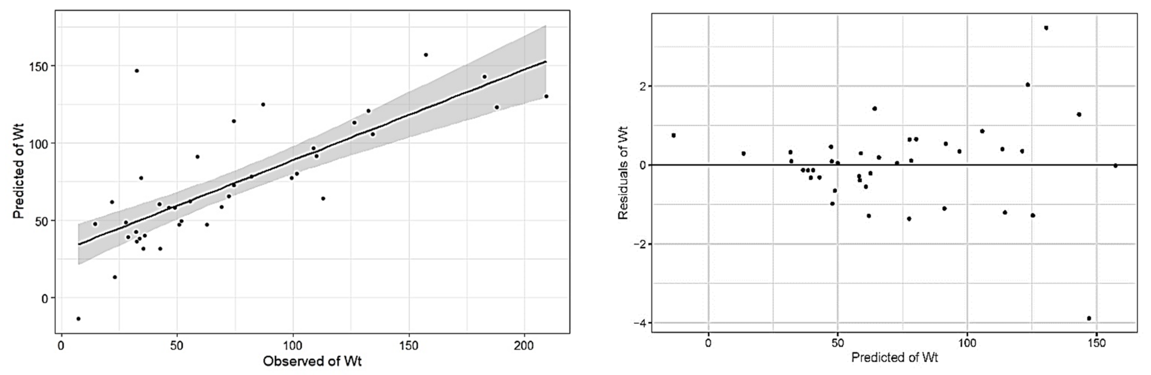
Figure 1. Location of the study area.
Drones 06 00148 g001
Figure 2. Technical roadmap for agave biomass estimation based on UAV images.
Drones 06 00148 g002
Figure 3. Correlation analysis.
Drones 06 00148 g003
Figure 4. Predicted versus observed values (left); predicted values versus residuals (right).
Drones 06 00148 g004
Figure 5. Wt map for Agave durangensis Gentry.
Drones 06 00148 g005
Table 1. Selected models for the estimation of green weight by components and total weight for Agave durangensis Gentry in the state of Durango.
ComponentModelParameterR2RMSE
Total green biomass (Wt) W t   =   β 1 D   +   β 2 D 2   +   β 3 D 2 A t   +   β 1 D   +   β 2 D 2   +   β 3 D 2 A t β 1 = 0.308681
β 2 = −0.00229
β 3 = 0.000018
0.7928.99
βn = regression coefficients; D = diameter of coverage; At = total height; R2 = coefficient of determination; RMSE = root-mean-square error.
Table 2. CANON S110NIR sensor image characteristics.
BandWavelength (µm)Spatial Resolution (cm)Abbreviation
Green0.54–0.575B1
Red0.65–0.685B2
Near-infrared0.78–0.905NIR
Table 4. Descriptive statistics of the variables of the agaves sampled in the field.
VariableMínimumMáximumMeanStandard Deviation
D (cm)54.4205126.0636.75
At (cm)46157101.5324.65
Wt (Kg)7.26209.3971.8148.73
D = diameter of coverage; At = total height; Wt = total green biomass.
Table 5. Regression model parameter.
ModelParameterR2RMSE
Wt = β0 + β1B1 + β2B2 + β3NDVI + β4GNDVI + β5EVI2 + β6SAVIβ0 = −528.170.5932.06 kg
β1 = −33.08
β2 = 36.43
β3 = 859.66
β4 = −11,476.71
β5 = 7035.82
β6 = −15.79
βn = regression coefficients; Wt = total green biomass; D = diameter of coverage; At = total height; R2 = coefficient of determination; RMSE = root-mean-square error.
Publisher’s Note: MDPI stays neutral with regard to jurisdictional claims in published maps and institutional affiliations.

