
SR-DeblurUGAN: An End-to-End Super-Resolution and Deblurring Model with High Performance

1
College of Information and Electrical Engineering, China Agricultural University, Beijing 100083, China
2
Yantai Research Institute, China Agricultural University, Yantai 264670, China
3
Century College, Beijing University of Posts and Telecommunications, Beijing 100876, China
*
Author to whom correspondence should be addressed.
†
These authors contributed equally to this work.
Drones 2022, 6(7), 162; https://0-doi-org.brum.beds.ac.uk/10.3390/drones6070162
Submission received: 3 May 2022
/
Revised: 13 June 2022
/
Accepted: 21 June 2022
/
Published: 27 June 2022
Abstract
:In this paper, we consider the difference in the abstraction level of features extracted by different perceptual layers and use a weighted perceptual loss-based generative adversarial network to deblur the UAV images, which removes the blur and restores the texture details of the images well. The perceptual loss is used as an objective evaluation index for training process monitoring and model selection, which eliminates the need for extensive manual comparison of the deblurring effect and facilitates model selection. The UNet jump connection structure facilitates the transfer of features across layers in the network, reduces the learning difficulty of the generator, and improves the stability of adversarial training.
1. Introduction
With the characteristics of low cost, high mobility and high imaging resolution, aerial photography by UAV (Unmanned Aerial Vehicle) plays an important role in disaster emergency rescue, power patrol and land resource investigation. In the process of acquiring UAV images, some of the images taken are blurred due to the mechanical vibration of the UAV, the rapid movement of ground targets, atmospheric turbulence effects, bokeh, etc. The blur caused by the relative motion between the UAV and the target is called motion blur, and the blur caused by objects imaged outside the focus of the camera is called bokeh blur. Most of the drones have poor wind resistance and are easily affected by wind during flight, making the flight attitude unstable. The blurred images captured are mainly caused by motion blur, which results in the loss of the detailed information of the images and has a great impact on applications that require important detail information, such as mis-matching in image feature matching and difficulty in accurately locating the contours of features. Therefore, deblurring the images captured by drones to recover a clear and detailed image is important for subsequent image processing.
Since the image displayed at the image receiving end is no longer the original image transmitted, the image effect has deteriorated significantly, providing obstacles for subsequent operations and calculations, etc., and causing instability in information transmission and inaccuracy of information. For this reason, the degraded image must be processed in order to recover the true original image and retain the complete information.
Image restoration has been a hot issue in image processing, especially in image repair and image deblurring to improve image resolution. High-resolution images are a fundamental and important part of many studies. For example, in geological exploration, the use of UAVs in mining and magnetic field discovery requires high-density, high-precision data that are not affected by vegetation, terrain, traffic, etc., where high-resolution images are an essential part [1]. Topographic data should also be flexible for high-resolution, low-cost transmission, which is also an important reference factor for geographic operations to be conducted [2]. In addition to conventional terrain, images of complex terrain not often seen in nature have a higher requirement for resolution because complex terrain may have a more abyssal significance for the study and discovery of geological conditions [3]. In archaeology, the need to take measurements from multiple angles (aerial and ground) and to combine aerial measurements with reconstructed structures and complex soil morphology places high demands on the resolution of the acquired images [4]. As research continues, through improvements in photogrammetry and identification, different cameras are developed with sensors that can provide different high resolutions and complementary spectral bands [5]. In ecology, the establishment of protected areas can better protect ecological environments and historical artifacts, so the use of drones to assess the level of protected areas and to monitor and measure sensitive areas has an important position, and this work relies on high-resolution images [6]. Furthermore, it is crucial to deal with biological invasions, and we need to effectively monitor invasive species monitoring, as they may affect the ecological balance and disrupt the biological habitat [7]. In terms of land management, the land cover should be assessed, such as bare ground, litter, green vegetation, destroyed vegetation, etc., to ensure that the land consolidation process is free from interference from other construction and mining operations [8]. The emergence of image restoration technology and its rapid development are due to the following reasons: firstly, the rapid development of computer technology and the increase in application fields have led to a deeper understanding of digital images; secondly, the current demand for high-quality images in agriculture, animal husbandry, forestry, industry and medicine is increasing. Image is also one of the important sources for people to obtain and exchange information in their daily life, so the application area of image recovery technology will definitely involve people’s daily work or life. As the area of human activities is expanding, the application area of image recovery technology is also bound to expand.
To obtain more accurate images, Suin, M. et al. proposed an inpainting approach for solving the problem of the inability of encoder layers to build complete and faithful embeddings of missing regions to improve on past methods, and good performance was obtained in multiple datasets [9]. Chen, J. et al. switched their ideas to solve the color image patching problem using pure quaternion matrices and proposed a new minimization problem that eliminates noise correlation, which was validated in multiple datasets [10]. Qiu, Z. et al. proposed the Dilated Convolution and Deformable Convolution Wasserstein Generative Adversarial Network (DDC-WGAN) to solve the problem, and this new approach was verified to have better performance than the traditional approach [11]. Peter, P. proposed a mask optimization network for data optimization in spatial picture-in-picture, with the improvement that a generator and a corresponding optimization network can be jointly trained, with the effect of accurately reflecting the image, achieving a breakthrough in quality and speed. Kumar, A. et al. proposed a new patching approach that can use GAN to focus on each aspect of image features, such as color and shape individually, and was validated in two datasets, achieving competitive performance [12]. Jam, J. et al. designed a loss model employing two encoders and proposed a recursive residual transition layer that achieved some technical progress in terms of bias and quality for image repair, which was well generalized on a stationary dataset [13]. Dervishaj, E. et al. proposed a GAN approach that uses matrix decomposition to learn potential factors with state-of-the-art results in image synthesis and image repair [14]. Park, Geonung et al. proposed the application of high-resolution images taken by drones for urban images, pointing out that reducing the number of variables in the classification does not produce significant changes in the initial versus optimized RF [15].
Image repair techniques have been extensively investigated and there have been significant advances in various aspects. Zheng, Haitian et al. proposed a new design of cascaded modulated GAN (CM-GAN) for large image breakage and information incompleteness, along with a training scheme for object perception to achieve better model results [16]. Dogan, Yahya et al. used the Recurrent Reverse Generator (CRG) architecture to refine the facial image recognition problem, which can use an iterative approach to solve the problem of missing parts in images, and trained their own specialized model to reach the industry-leading level [17]. Lu, W. et al. proposed EXE-GAN, which partially solves the face image drawing problem using a diverse and interactive face inpainting framework, experimenting on publicly available datasets and demonstrating its advantages in terms of face repair quality and diversity. Zhao, Y. et al. used a reference to another image to recover the original mutilated image, relying on monocular depth estimation for a more principled training that requires heuristic plane assumptions, obtained optimal levels on a fixed dataset, and can effectively solve problems with a large range of image residuals [18]. Rezki, A. M. et al. proposed an improved patch classification algorithm with the advantage of not requiring a reference, which is very suitable for spray paint evaluation without a reference and was performed on the TUM-IID database. After analysis, the results were found to have better results than existing algorithms [19]. Hudagi, M. R. et al. proposed a hybrid image restoration approach that can effectively repair missing images by removing unwanted objects from the image, achieving a maximum PSNR of 38.14 dB, a maximum SDME of 75.70 dB, and a maximum SSIM of 0.983 as the leading effect [20]. Li, W. et al. proposed a transformer-based large-aperture inpainting model that combines the advantages of transformers and convolution to give higher realism and diversity to images, achieving state-of-the-art performance in multiple datasets [21].
From the above analysis, it can be found that many scholars have proposed many solutions to the problem of image resolution enhancement and image deblurring, but the following shortcomings still exist in this field of research:
- The model is still inadequate in extracting subtle features and cannot capture subtle differences in color and shape in images.
- Image repair sometimes produces distorted parts that cannot be strictly embedded with the surrounding pixels.
- Inability to generate reasonable images that achieve good results in repairing large gaps.
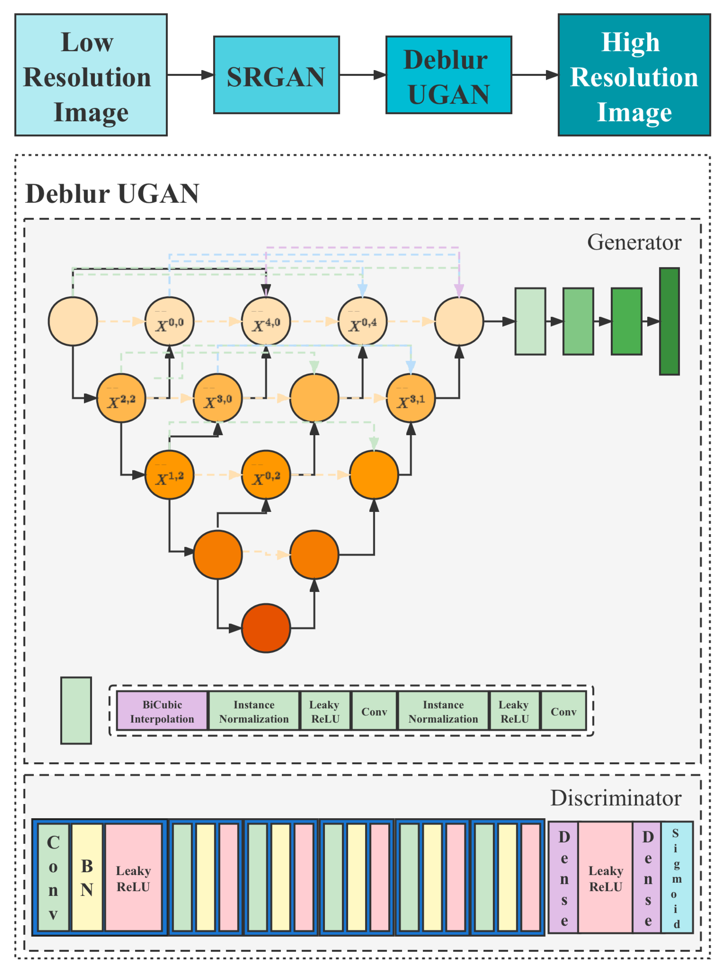
Therefore, in this paper, we propose the SR-DeblurUGAN model, whose operation process is: firstly, the image is enlarged in resolution, then the color is filled, and then the image is corrected by the discriminator, and finally, the image is reconstructed into a high-resolution image. It can reduce the amount of transmission data of UAV aerial photography and improve the battery utilization of UAV while ensuring the image quality. The structure of our model is shown in Figure 1.
2. Related Works
2.1. Overall
Among the more influential generative models are VAE [22], PixelCNN [23], Glow [24], and GAN [25]. The great success of GAN in image generation undoubtedly depends on the fact that GAN keeps improving its modeling ability under gaming and finally achieves image generation with falsehoods. It consists of two neural networks, a generator and a discriminator, where the generator tries to generate real samples that deceive the discriminator, and the discriminator tries to distinguish between real and generated samples. This adversarial game makes the generator and discriminator continuously improve their performance, and the generator can achieve false output after reaching the Nash equilibrium. However, this Nash equilibrium exists only in theory, and the actual GAN training is accompanied by some problematic limitations. One is GAN training instability, and the other is pattern collapse.
2.1.1. CGAN
In the original GAN, there is no control over what is to be generated because the output depends only on the random noise. We can add the conditional input c to the random noise z so that the generated image is defined by . This is CGAN [26], where it is usually sufficient to connect the conditional input vector c directly to the noise vector z, and to use the resulting vector as is as input to the generator, just as it was in the original GAN. The condition c can be the class of the image, a property of the object or a textual description embedded in the image that one wants to generate, or even a picture.
2.1.2. ACGAN
To provide more auxiliary information and allow semi-supervised learning, additional auxiliary classifiers can be added to the discriminator in order to optimize the model on the original task as well as on the additional tasks. The architecture of this approach is shown in the figure below, where C is the auxiliary classifier. Adding auxiliary classifiers allows us to use pre-trained models (e.g., image classifiers trained on ImageNet), and experiments in ACGAN [27] demonstrate that this approach can help generate sharper images as well as mitigate pattern collapse problems. The use of auxiliary classifiers can also be applied in text-to-image synthesis and image-to-image conversion.
2.1.3. GAN Combined with Encoder
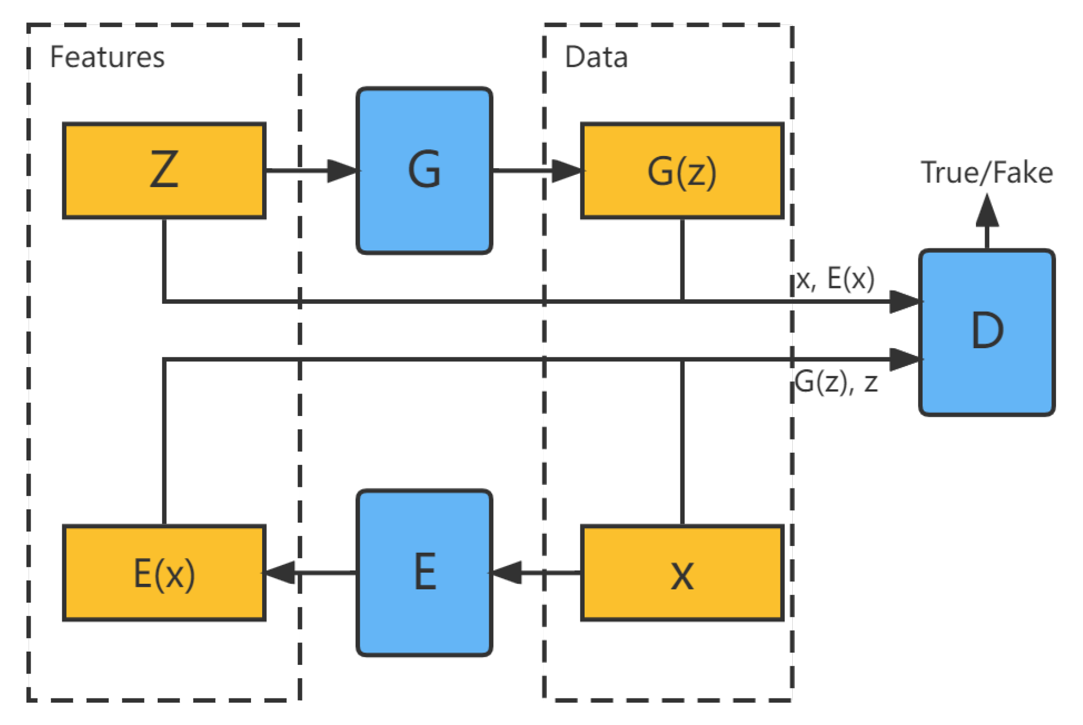
Although GAN can transform the noise vector z into a synthetic data sample , it does not allow for inverse transformations. If the noise distribution is considered as a potential feature space of data samples, GAN lacks the ability to map data samples x to potential features z. To allow such a mapping, BiGAN [28] adds encoder E to the original GAN, as shown in Figure 2.
Let be the data space and be the potential feature space, encoder E takes as input and produces a feature vector as output. The modified discriminator D computes by taking both data samples and feature vectors as inputs, where means that the samples are real while means that the data are generated by G. Expressed in a mathematical equation as:
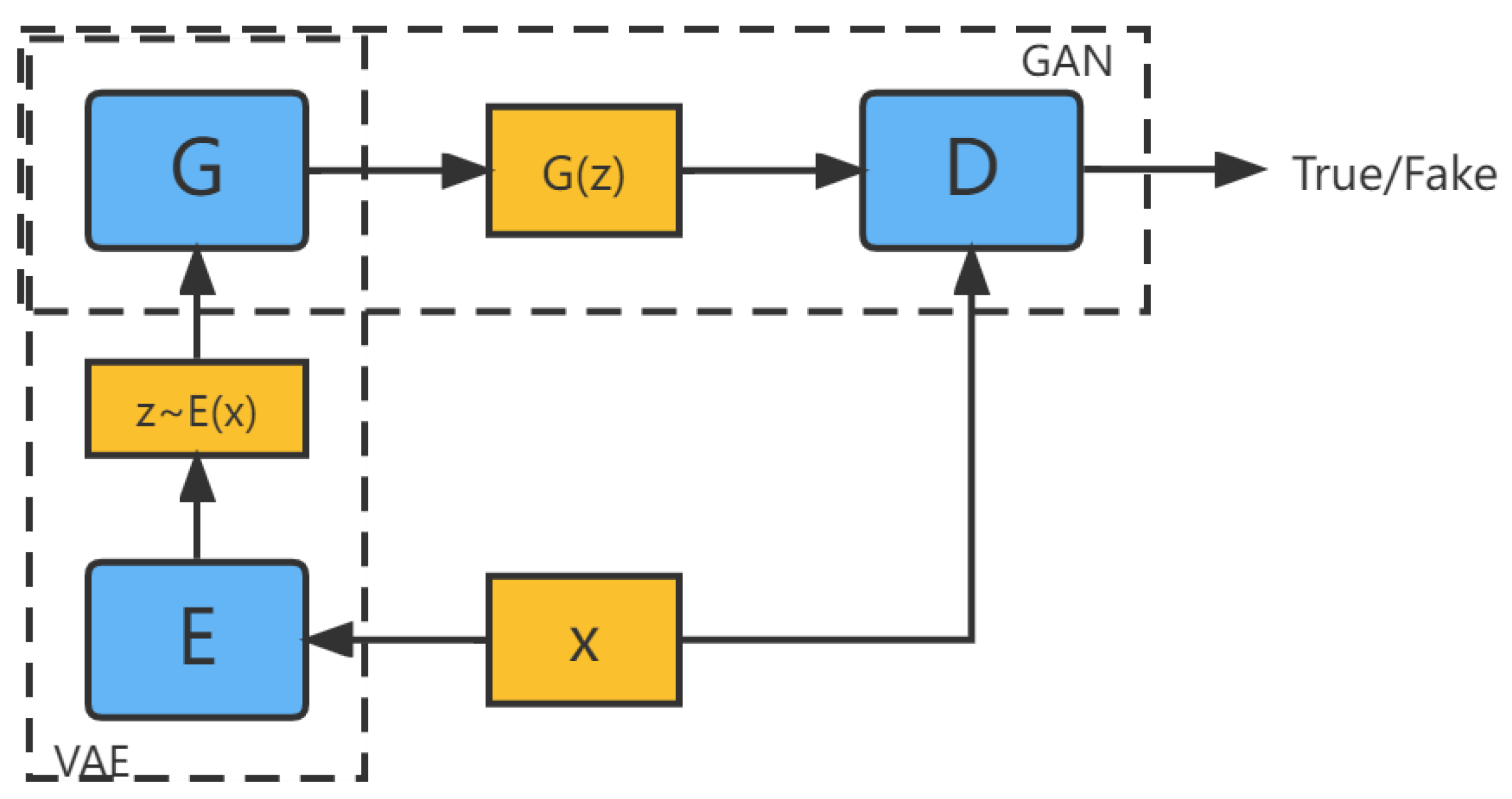
2.1.4. VAE-GAN
2.2. GAN in Image Generation Tasks
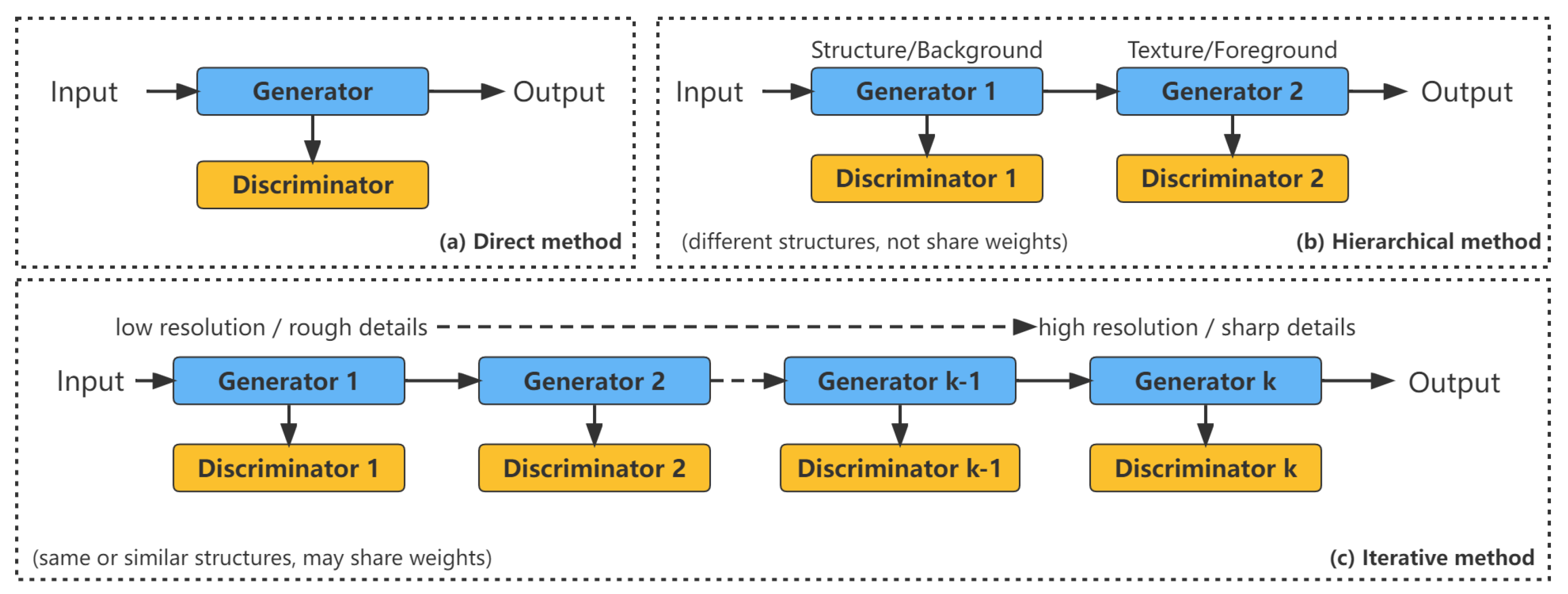
The main methods of GAN in image generation are direct methods, connection methods and iterative methods, which can be shown in Figure 4.
Distinguish an image generation method by the number of generators and discriminators it has.
2.2.1. Direct Methods
All methods under this category follow the principle of using a generator and a discriminator in their models, and the structure of the generator and discriminator is straightforward and without branches. Many of the earliest GAN models belong to this category, such as GAN, DCGAN [30], ImprovedGAN [31], InfoGAN [32], f-GAN [33] and GANINT-CLS [34]. Among them, DCGAN is one of the most classical ones and its structure is used by many later models. The general building blocks used in DCGAN are shown below, where the generator uses deconvolution, batch normalization and ReLU activation, while the discriminator uses convolution, batch normalization and LeakyReLU activation, which are nowadays used by many GAN model network designs. This approach is relatively more straightforward to design and implement than the hierarchical and iterative approaches and usually yields good results.
2.2.2. Hierarchical Methods
In contrast to the direct methods, the algorithms under the layered approach use two generators and two discriminators in their models, where the different generators have different purposes. The idea behind these methods is to divide the image into two parts, such as “style and structure” and “foreground and background”. The relationship between the two generators can be in parallel or in series.
2.2.3. Iterative Methods
The iterative method differs from the hierarchical method in that, first, instead of using two different generators performing different roles, the models in this category use multiple generators with similar or even the same structure, and they generate images from coarse to fine, with each generator regenerating the details of the result. When using the same structure in the generators, iterative methods can use weight sharing among the generators, while hierarchical methods usually cannot.
LAPGAN is the first GAN that uses the Laplace pyramid to generate images from coarse to fine using iterative methods. Multiple generators in LAPGAN perform the same task: acquiring the image from the previous generator and taking the noise vector as input, and then outputting the details that make the image sharper when added back to the input image (residual image). The only difference between these generator structures is the size of the input/output dimensions, with the exception that the lowest-level generator takes only the noise vector as input and outputs the image. LAPGAN outperforms the original GAN and shows that iterative methods can generate sharper images than direct methods.
2.2.4. Other Methods
Unlike the other methods mentioned earlier, PPGN [35] uses activation maximization to generate images, which is based on samples previously learned using denoising autoencoders (DAE) [36]. In order to generate images conditioned on a specific class label y, instead of using a feed-forward approach (e.g., a recurrent method can be considered as feed-forward if it is expanded through time), the PPGN optimization process finds the input z for the generator, which makes the output image highly activated for a certain neuron in another pre-trained classifier (the neuron in the output layer corresponding to its class label y).
3. Materials and Methods
3.1. Dataset Analysis
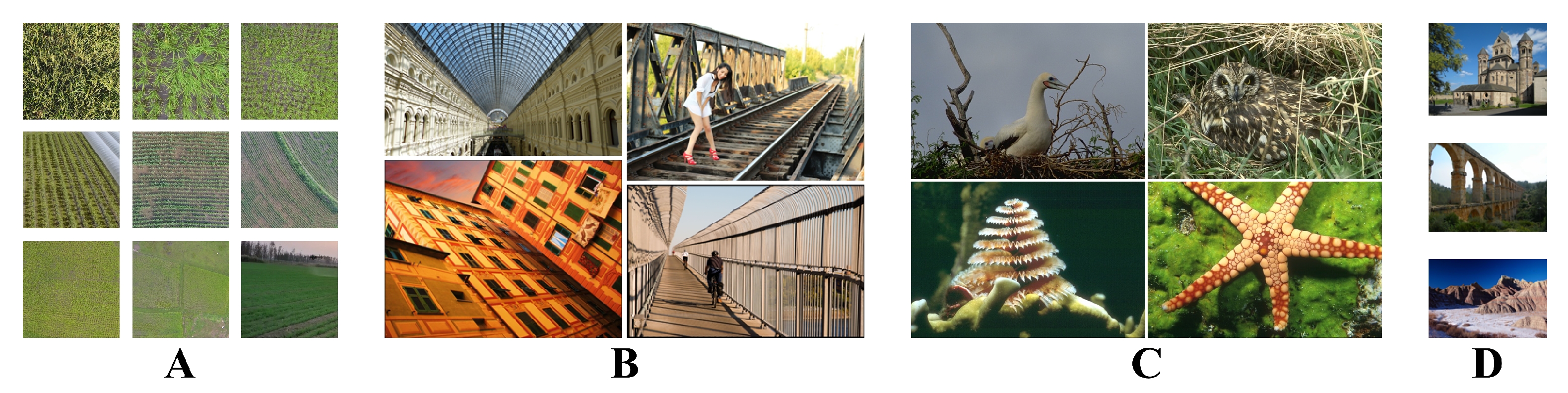
The datasets used in this paper have multiple sources. Testing images of four datasets (agricultural datasets taken by drones, Urban 100, BSD 100, Sun-Hays 80). All the images were cropped according to the desired super-resolution factor. This avoids misalignment of the groundtruth high-resolution images and the super-resolved images. The details are as follows:
- Agricultural dataset collected in Shahe Town, Laizhou City, Yantai City, Shandong Province, China, at 09:00–14:00 and 16:00–18:00 on 8 April 2022. The collected images are shown in Figure 5A. A drone was equipped with a Canon 5D camera (stabilized by a tripod). This camera acquires solid color images at 8-bit resolution. The acquisition is performed automatically at a predetermined cadence during flight preparation. The system uses autonomous ultrasonic sensor flight technology to reduce the risk of accidents. The system includes a ground control radio connected to a smartphone with a range of 5 km (without obstacles) under normal conditions.
- The Urban100 dataset contains 100 images of urban scenes. It is commonly used as a test set to evaluate the performance of super-resolution models.
- The BSD 100 dataset is a dataset that provides an empirical basis for the study of image segmentation and boundary detection, containing 1000 hand-labeled segments of 1000 Corel dataset images from 30 human subjects, half of which were obtained by presenting color images to the subjects; the other half were obtained by presenting grayscale images. A common benchmark based on these data includes all grayscale and color segmentations of the 300 images. The BSD 300 dataset is divided into 200 training images and 100 side views, and the ground truth is divided into two folders, color and gray, which in turn have subfolders named after the marker id (uid), containing segmentation information provided by each marker. These folders have subfolders named by marker id (uid), which contain segmentation information provided by each marker, named by image id, and saved as .seg files. The dataset was released in 2001 by the University of California, Berkeley.
- The Sun-Hays 80 dataset is a dataset that has been used for super-resolution image studies to compare and find relevant scenes in image databases using global scene descriptions that provide ideal example textures to constrain image sampling to problems that are more predictive of explicit scene matching compared to internal image statistics for super-resolution tasks. We used patch-based texture transfer techniques and generated phantom texture details after comparing the publisher’s super-resolution images with other methods to draw conclusions. This dataset was released institutionally by Brown University in 2012.
3.2. Dataset Augmentation
Since running the SRGAN model is very memory intensive, it consumes too many hardware resources to train the machine with large images; moreover, the number of images in the training set is very small. Therefore, in this paper, we randomly crop a small piece of the low-resolution image and the high-resolution image “at the same location” for training. On the one hand, it expands the number of images in the dataset and prevents overfitting. On the other hand, it reduces the memory consumption of the model. After this operation, there are random rotation and random flip operations to expand the dataset. In the end, the resulting training set amounted to 3800 images.
3.3. Proposed Model
3.3.1. Generator
For image transformation problems, networks with an encoding–decoding structure are generally used. The coding and decoding phases have a symmetric structure so that the output and input dimensions of the network are consistent. In the coding stage, the features are extracted gradually using convolutional layers, and the feature map resolution is gradually reduced by pooling layers. Then, the feature details and spatial location information are gradually recovered through the decoding process after reaching the bottleneck layer. For image deblurring, there are some common features between the input blurred image and the output deblurred image, the tone of the image should be the same, and the edges of the image should be similar.
The Unet [37] model is different from the common encoding–decoding network in that it has a jump connection structure, and the features extracted in the encoding stage can bypass the bottleneck layer to reach the decoding stage, which makes the features recovered in the decoding stage more detailed and helps to reduce the difficulty of generator learning. In this paper, we make two main improvements based on Unet:
- Adding a batch normalization layer after the convolutional layer but not for the output layer, which is beneficial to the rapid convergence of the deep network and, to a certain extent, to the effect of regularization, reducing the risk of overfitting, etc.
- The number of feature maps is halved, which significantly reduces the number of network parameters, saves computational resources, improves training and prediction speed, and allows inputting larger sample batches for training.
The modified Unet network has 8 convolutional layers and 4 pooling layers in the coding stage, 4 deconvolutional layers and 8 convolutional layers in the decoding stage, and the size of the feature map becomes twice as large as the original one for each deconvolutional layer, and the size of the convolutional kernel is .
3.3.2. Discriminator
The discriminator is generally an ordinary multilayer convolutional neural network. The input sample is the probability value of the real sample. The higher the probability value, the higher the probability that the discriminator considers the input sample as the real sample. In this paper, the discriminator outputs not a single probability, but a patch of probability values, using the PatchGAN [38] model. Each value in the patch represents its receptive field, which corresponds to the probability that the local image block is from the real sample, which is helpful to recover as much high-frequency information as possible in each receptive field and make the deblurred image details clearer. In this paper, the discriminator is an ordinary multilayer convolutional network with , and its corresponding input image perceptual field size is 64, i.e., each value in the block represents the probability that a block of size in the input image is from the real sample. The structure of the discriminator is shown in Figure 1, where each bar represents a sequential operation consisting of a convolutional layer, a batch normalization layer, and a nonlinear activation layer. The size of the convolutional kernel is , the nonlinear activation function uses LeakyReLU [39], and the slope is set to .
4. Experiments
4.1. Overall
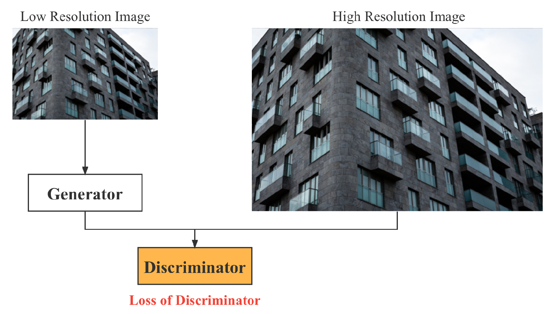
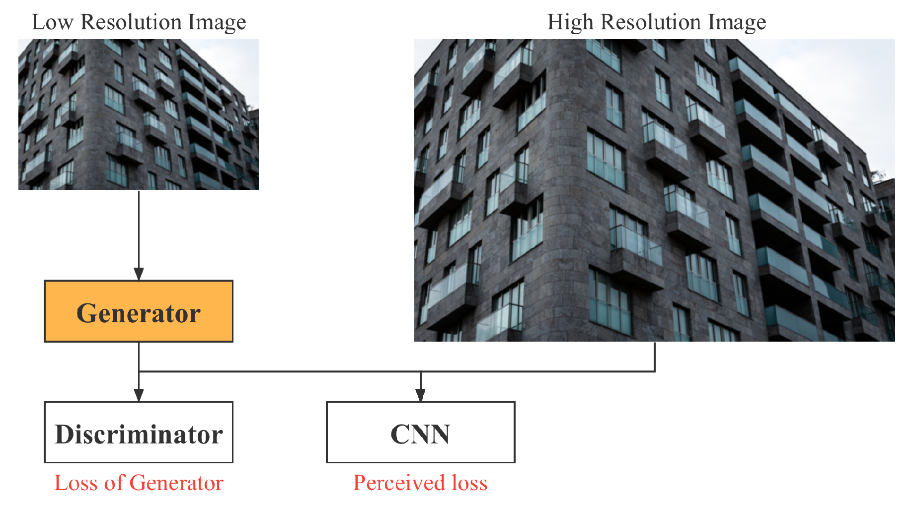
The process of adversarial training is as follows: the discriminator is trained first, then the generator is trained, and so on alternately. The discriminator training process is shown in Figure 6, and the generator training process is shown in Figure 7.
The transparent box in the figure indicates the frozen network, where the network parameters are not updated during training; only the network in the orange box is involved in training. The discriminator uses cross-entropy as the loss function, the labels of the real samples are set to 1, and the labels of the fake samples output by the generator are set to 0. When the generator is trained, the discriminator is frozen and the labels of the generator output are set to 1, which are used to deceive the discriminator. The loss function of the generator is the sum of two parts; the first part is the perceptual loss obtained by the CNN, and the other part is the loss from the failure to deceive the discriminator.
4.2. Experiment Parameters and Platform
The test device is a desktop computer with a Core i9-10900k CPU and Nvidia RTX3080 GPU. In the training process, the experiments were run on Ubuntu 20.14, using the Python programming language, and the model implementation was based on the PyTorch framework. The number of learning rounds was set to 150, and the network was optimized using the stochastic gradient descent algorithm, where the initial learning rate is .
4.3. Experiment Metrics
The traditional methods mainly use the peak signal-to-noise ratio (PSNR), structural similarity index and other image quality evaluation indexes or are directly determined by human visual perception. However, PSNR ignores the influence of image content on human eyes and cannot fully reflect the image quality, which leads to stopping training too early or too late. SSIM can achieve better quality evaluation results than PSNR but cannot completely solve the problem of PSNR. SSIM can achieve better quality evaluation results than PSNR but does not completely solve the problem of PSNR. For both PSNR and SSIM methods, it is possible that there are two signals with the same structural similarity to the same original signal, but the subjective quality still differs, which is difficult to automate by human visual analysis, and the workload is high. The perceptual loss function measures the difference between the generated image and the target image in terms of high-level image features, and the image reconstructed using perceptual loss is more detailed and semantically consistent with human visual perception than calculating the loss at the lowest level of grayscale values. For example, if two images are identical and one of them is shifted by one pixel, the loss calculated using image grayscale values will be much larger, but at the more abstract feature level, the perceptual loss remains almost unchanged.
Regarding the model speed, in this paper, 100 images were processed and timed in a single succession until all test set data were inferred. The average inference time per 100 images was found, and thus the FPS (Frames Per Second) was found.
4.3.1. Peak Signal-to-Noise Ratio (PSNR)
The PSNR is generally an engineering project used between the maximum signal and the background noise. Usually, after image compression, the output image is usually different from the original image to some extent. In order to measure the quality of the processed image, we usually refer to the PSNR value to measure whether a processing procedure is satisfactory or not. It is the logarithmic value of the mean squared error between the original image and the processed image relative to (the square of the maximum value of the signal, n being the number of bits per sample) and is measured in dB.
Since perceptual loss is closer to human visual perception in evaluating the details and semantics of reconstructed images, this paper uses perceptual loss as a metric for model selection. The network weights are selected by analyzing the direction and change of perceptual loss curves on the validation and training sets.
Peak signal-to-noise ratio is often used as a measure of signal reconstruction quality in areas such as image compression, and it is often defined simply by the mean squared error (MSE). For two monochrome images I and K, if one is a noise approximation of the other, then their MSEs are defined as:
where is the maximum value indicating the color of the image point, which is 255 if each sample point is represented by 8 bits.
4.3.2. Structural Similarity Index
The structural similarity index (SSIM) is a metric used to quantify the structural similarity between two images. Unlike the L2 loss function, SSIM is modeled after the Human Visual System (HVS), which implements the theory related to structural similarity and is sensitive to the perception of local structural changes in an image. SSIM quantifies the properties of an image in terms of luminance, contrast and structure, using the mean to estimate luminance, variance to estimate contrast and covariance to estimate the degree of structural similarity. The SSIM values range from 0 to 1, with larger values representing more similar images. The SSIM value is 1 if the two images are identical. Given two images x, y, the luminance, contrast and structure between them are shown in the following equations.
where is the mean of x, is the variance of x, is the mean of y, is the variance of y, is the covariance of x and y, are two constants used to maintain stability and avoid division by zero, and L is the range of pixel values, indicating that the L value for a B-bit image is . In general, for uint8 data, the maximum pixel value is 255, and for floating-point data, the maximum pixel value is 1. In general, .
5. Results and Discussion
5.1. Results
From Table 1, we can see that the PSNR and SSIM of our method are higher than those of deblurGAN, which means that this method is richer in details after deblurring, and deblurGAN loses some texture information after deblurring.
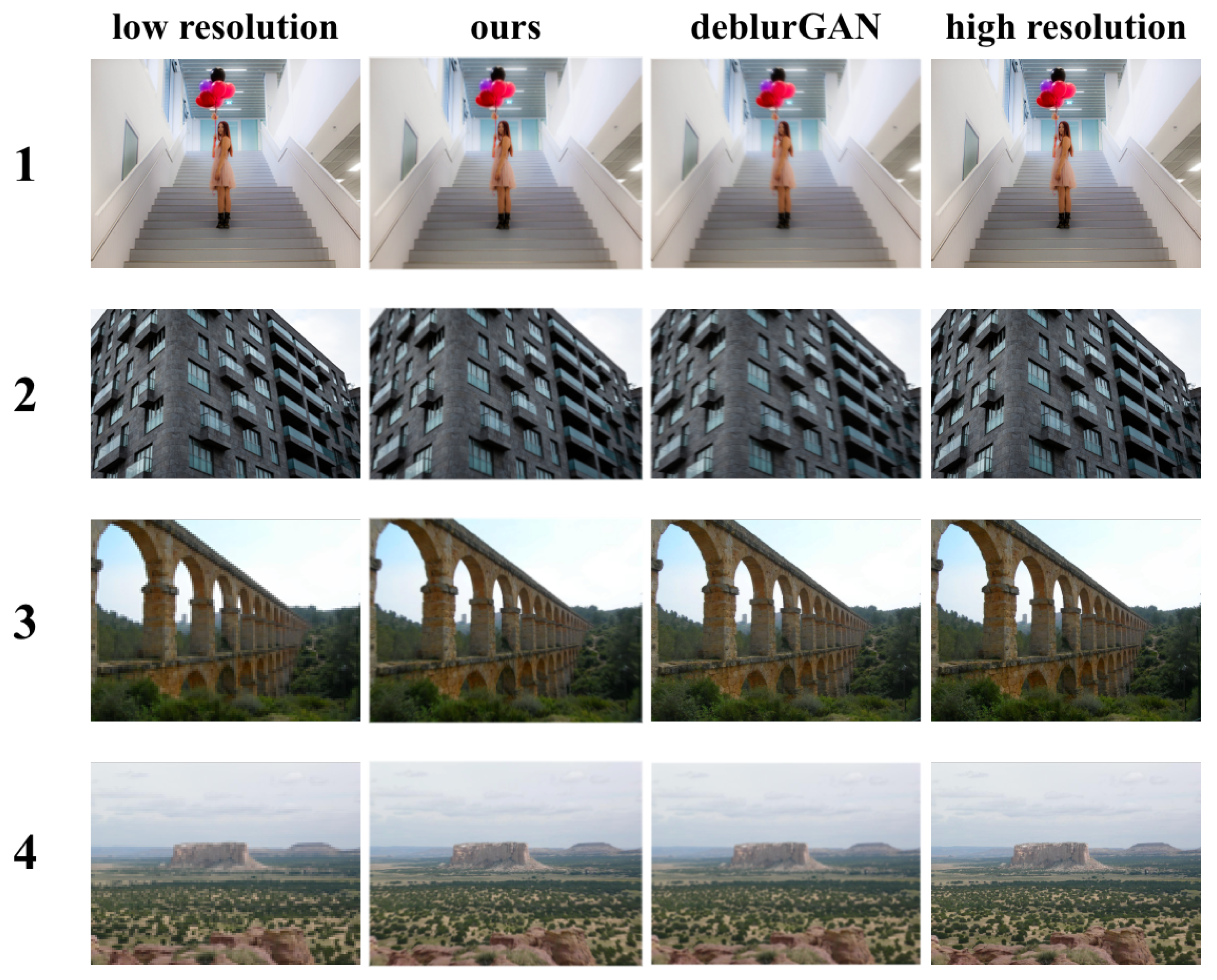
Figure 8 shows a comparison of before and after the application of various models.
From the above figure, we can see that the perceptual loss of this method is lower than that of other models, which means that the recovered images are semantically closer to the subjective judgment of image quality. deblurGAN does not take into account the difference in the abstraction level of the features proposed by different perceptual layers and does not constrain the low-level perceptual layers enough to extract detailed features, which makes the recovered images still smooth. It can be seen that the deblurred image by the model highlighted in this question is consistent with the original image in terms of tone, and the texture information is richer and the details are clearer.
The experimental results show that the method in this paper has the following advantages:
- More effective recovery of image details;
- Lower deblurring processing time.
5.2. Validation on More Channels
In the above experimental results, we follow the traditional approach to super-resolve (super-resolve) color images. Specifically, we first convert the color image to space. The SR algorithm is applied to the Y channel only, while the and channels are interpolated by bicubic interpolation. In this section, we try to consider all three channels in this process and verify the model performance.
The model in this paper can accept more channels without changing the learning mechanism and the network signal. In particular, by setting the input channel to , it can easily handle three channels simultaneously. The experimental results are shown in Table 2.
From the experimental results, we can see that from the model proposed in this paper, the visual effect of the transmitted image is not much different from the original effect, and the amount of transmitted data is smaller, the transmission time is shorter, and the model is more robust.
5.3. Application on Edge Computing
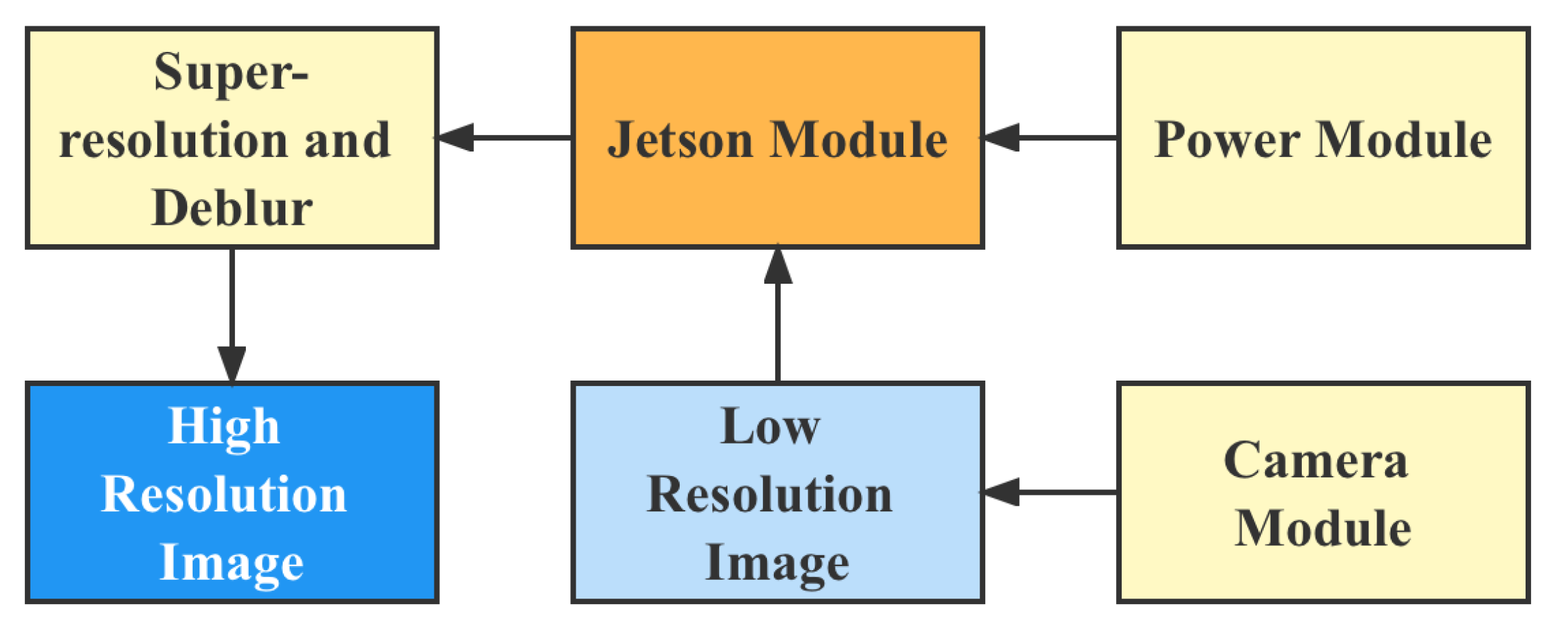
In order to deploy the SRUGAN model proposed in this paper in a practical application scenario, we developed an edge computing device based on Jetson, whose system architecture is shown in Figure 9.
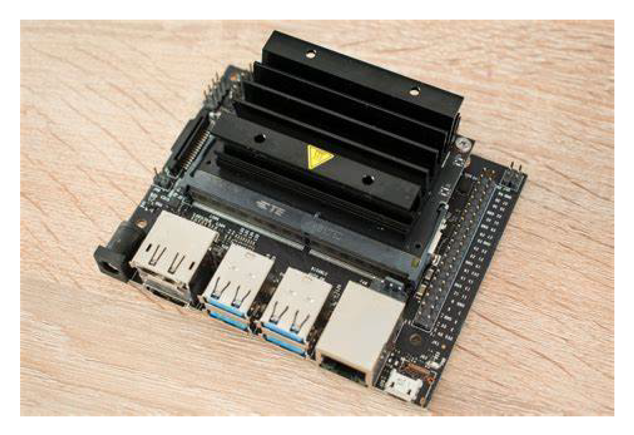
The Wifi module acquires the low-resolution raw images transmitted by the UAV, and the Jetson operational logic board performs the image super-resolve and deblurring operations locally. The display module can display the processing results in real-time. A physical diagram of the device is shown in Figure 10.
We have protected the entire computational body with aluminum. The weight of this device is less than 700 g, which is less than the weight of a normal DSLR camera, such as the Canon 5D. This allows the device to be easily mounted on a drone. With this device, we can capture optimized images directly on the drone and transmit them to the local host.
6. Conclusions
In this paper, we consider the difference in the abstraction level of features extracted by different perceptual layers and use a weighted perceptual loss-based generative adversarial network to deblur the UAV images, which removes the blur and restores the texture details of the images well. The perceptual loss is used as an objective evaluation index for training process monitoring and model selection, which eliminates the need for extensive manual comparison of the deblurring effect and facilitates model selection. The UNet jump connection structure facilitates the transfer of features across layers in the network, reduces the learning difficulty of the generator, and improves the stability of adversarial training. At the same time, this structure helps to extract subtle information from the images.
GANs tend to show some inconsistencies in performance. Therefore, in this paper, we use various datasets, including open-source datasets and self-harvested agricultural datasets, to test them, and the experimental results show that the proposed model achieves stable performance on these datasets.
In the future, we will continue to study the structure of the generator network to ensure the recovery of image quality and further improve the prediction efficiency.
Author Contributions
Conceptualization, Y.X.; methodology, Y.X. and J.Z.; validation, Y.X.; formal analysis, J.Z.; writing—original draft preparation, Y.X., Y.W. and J.Y.; writing—review and editing, W.C. and Y.W.; visualization, Y.X.; funding acquisition, Q.W. All authors have read and agreed to the published version of the manuscript.
Funding
This research received no external funding.
Institutional Review Board Statement
Not applicable.
Informed Consent Statement
Not applicable.
Data Availability Statement
Not applicable.
Conflicts of Interest
The authors declare no conflict of interest.
References
- Porras, D.; Carrasco, J.; Carrasco, P.; Alfageme, S.; Gonzalez-Aguilera, D.; Lopez Guijarro, R. Drone Magnetometry in Mining Research. An Application in the Study of Triassic Cu;Co;Ni Mineralizations in the Estancias Mountain Range, Almería (Spain). Drones 2021, 5, 151. [Google Scholar] [CrossRef]
- Liu, X.; Lian, X.; Yang, W.; Wang, F.; Han, Y.; Zhang, Y. Accuracy Assessment of a UAV Direct Georeferencing Method and Impact of the Configuration of Ground Control Points. Drones 2022, 6, 30. [Google Scholar] [CrossRef]
- Shelekhov, A.; Afanasiev, A.; Shelekhova, E.; Kobzev, A.; Tel’minov, A.; Molchunov, A.; Poplevina, O. Low-Altitude Sensing of Urban Atmospheric Turbulence with UAV. Drones 2022, 6, 61. [Google Scholar] [CrossRef]
- Orsini, C.; Benozzi, E.; Williams, V.; Rossi, P.; Mancini, F. UAV Photogrammetry and GIS Interpretations of Extended Archaeological Contexts: The Case of Tacuil in the Calchaquiacute; Area (Argentina). Drones 2022, 6, 31. [Google Scholar] [CrossRef]
- Fiz, J.I.; Martín, P.M.; Cuesta, R.; Subías, E.; Codina, D.; Cartes, A. Examples and Results of Aerial Photogrammetry in Archeology with UAV: Geometric Documentation, High Resolution Multispectral Analysis, Models and 3D Printing. Drones 2022, 6, 59. [Google Scholar] [CrossRef]
- Bollard, B.; Doshi, A.; Gilbert, N.; Poirot, C.; Gillman, L. Drone Technology for Monitoring Protected Areas in Remote and Fragile Environments. Drones 2022, 6, 42. [Google Scholar] [CrossRef]
- Pádua, L.; Antao-Geraldes, A.M.; Sousa, J.J.; Rodrigues, M.A.; Oliveira, V.; Santos, D.; Miguens, M.F.P.; Castro, J.P. Water Hyacinth (Eichhornia crassipes) Detection Using Coarse and High Resolution Multispectral Data. Drones 2022, 6, 47. [Google Scholar] [CrossRef]
- Miller, Z.; Hupy, J.; Hubbard, S.; Shao, G. Precise Quantification of Land Cover before and after Planned Disturbance Events with UAS-Derived Imagery. Drones 2022, 6, 52. [Google Scholar] [CrossRef]
- Suin, M.; Purohit, K.; Rajagopalan, A.N. Adaptive Image Inpainting. arXiv 2022, arXiv:2201.00177. [Google Scholar]
- Chen, J.; Ng, M.K. Color Image Inpainting via Robust Pure Quaternion Matrix Completion: Error Bound and Weighted Loss. arXiv 2022, arXiv:2202.02063. [Google Scholar]
- Qiu, Z.; Yuan, L.; Liu, L.; Yuan, Z.; Chen, T.; Xiao, Z. Generative Image Inpainting with Dilated Deformable Convolution. J. Circuits Syst. Comput. 2022, 31, 2250114. [Google Scholar] [CrossRef]
- Kumar, A.; Tamboli, D.; Pande, S.; Banerjee, B. RSINet: Inpainting Remotely Sensed Images Using Triple GAN Framework. arXiv 2022, arXiv:2202.05988. [Google Scholar]
- Jam, J.; Kendrick, C.; Drouard, V.; Walker, K.; Yap, M.H. V-LinkNet: Learning Contextual Inpainting Across Latent Space of Generative Adversarial Network. arXiv 2022, arXiv:2201.00323. [Google Scholar]
- Dervishaj, E.; Cremonesi, P. GAN-based Matrix Factorization for Recommender Systems. In Proceedings of the 37th ACM/SIGAPP Symposium on Applied Computing, Virtual Event, 25–29 April 2022. [Google Scholar]
- Park, G.; Park, K.; Song, B.; Lee, H. Analyzing Impact of Types of UAV-Derived Images on the Object-Based Classification of Land Cover in an Urban Area. Drones 2022, 6, 71. [Google Scholar] [CrossRef]
- Zheng, H.; Lin, Z.; Lu, J.; Cohen, S.; Shechtman, E.; Barnes, C.; Zhang, J.; Xu, N.; Amirghodsi, S.; Luo, J. CM-GAN: Image Inpainting with Cascaded Modulation GAN and Object-Aware Training. arXiv 2022, arXiv:2203.11947. [Google Scholar]
- Dogan, Y.; Keles, H.Y. Iterative facial image inpainting based on an encoder-generator architecture. Neural Comput. Appl. 2022, 34, 10001–10021. [Google Scholar] [CrossRef]
- Zhao, Y.; Barnes, C.; Zhou, Y.; Shechtman, E.; Amirghodsi, S.; Fowlkes, C. GeoFill: Reference-Based Image Inpainting of Scenes with Complex Geometry. arXiv 2022, arXiv:2201.08131. [Google Scholar]
- Rezki, A.M.; Serir, A.; Beghdadi, A. Blind image inpainting quality assessment using local features continuity. Multimed. Tools Appl. 2022, 81, 9225–9244. [Google Scholar] [CrossRef]
- Hudagi, M.R.; Soma, S.; Biradar, R.L. Bayes-Probabilistic-Based Fusion Method for Image Inpainting. Int. J. Pattern Recognit. Artif. Intell. 2022, 36, 2254008. [Google Scholar] [CrossRef]
- Li, W.; Lin, Z.; Zhou, K.; Qi, L.; Wang, Y.; Jia, J. MAT: Mask-Aware Transformer for Large Hole Image Inpainting. In Proceedings of the IEEE/CVF Conference on Computer Vision and Pattern Recognition, New Orleans, LA, USA, 19–24 June 2022. [Google Scholar]
- Kingma, D.P.; Welling, M. Auto-encoding variational bayes. arXiv 2013, arXiv:1312.6114. [Google Scholar]
- Van den Oord, A.; Kalchbrenner, N.; Espeholt, L.; Vinyals, O.; Graves, A. Conditional image generation with pixelcnn decoders. In Proceedings of the Thirtieth Conference on Neural Information Processing Systems, Barcelona, Spain, 9 December 2016; Volume 29. [Google Scholar]
- Kingma, D.P.; Dhariwal, P. Glow: Generative flow with invertible 1x1 convolutions. In Proceedings of the 2018 Conference on Neural Information Processing Systems, Montreal, QC, Canada, 3–8 December 2018; Volume 31. [Google Scholar]
- Goodfellow, I.J.; Pouget-Abadie, J.; Mirza, M.; Xu, B.; Warde-Farley, D.; Ozair, S.; Courville, A.; Bengio, Y. Generative Adversarial Networks. In Advances in Neural Information Processing Systems; The MIT Press: London, UK, 2014; Volume 3, pp. 2672–2680. [Google Scholar]
- Mirza, M.; Osindero, S. Conditional generative adversarial nets. arXiv 2014, arXiv:1411.1784. [Google Scholar]
- Odena, A.; Olah, C.; Shlens, J. Conditional image synthesis with auxiliary classifier gans. In Proceedings of the International Conference on Machine Learning, Sydney, Australia, 6–11 August 2017; pp. 2642–2651. [Google Scholar]
- Donahue, J.; Krähenbühl, P.; Darrell, T. Adversarial feature learning. arXiv 2016, arXiv:1605.09782. [Google Scholar]
- Larsen, A.B.L.; Sønderby, S.K.; Larochelle, H.; Winther, O. Autoencoding beyond pixels using a learned similarity metric. In Proceedings of the International Conference on Machine Learning, New York, NY, USA, 20–22 June 2016; pp. 1558–1566. [Google Scholar]
- Radford, A.; Metz, L.; Chintala, S. Unsupervised representation learning with deep convolutional generative adversarial networks. arXiv 2015, arXiv:1511.06434. [Google Scholar]
- Salimans, T.; Goodfellow, I.; Zaremba, W.; Cheung, V.; Radford, A.; Chen, X. Improved techniques for training gans. In Proceedings of the Thirtieth Conference on Neural Information Processing Systems, Barcelona, Spain, 9 December 2016; Volume 29. [Google Scholar]
- Chen, X.; Duan, Y.; Houthooft, R.; Schulman, J.; Sutskever, I.; Abbeel, P. Infogan: Interpretable representation learning by information maximizing generative adversarial nets. In Proceedings of the Thirtieth Conference on Neural Information Processing Systems, Barcelona, Spain, 9 December 2016; Volume 29. [Google Scholar]
- Nowozin, S.; Cseke, B.; Tomioka, R. f-gan: Training generative neural samplers using variational divergence minimization. In Proceedings of the Thirtieth Conference on Neural Information Processing Systems, Barcelona, Spain, 9 December 2016; Volume 29. [Google Scholar]
- Reed, S.; Akata, Z.; Yan, X.; Logeswaran, L.; Schiele, B.; Lee, H. Generative adversarial text to image synthesis. In Proceedings of the International Conference on Machine Learning, New York, NY, USA, 20–22 June 2016; pp. 1060–1069. [Google Scholar]
- Nguyen, A.; Clune, J.; Bengio, Y.; Dosovitskiy, A.; Yosinski, J. Plug & play generative networks: Conditional iterative generation of images in latent space. In Proceedings of the IEEE Conference on Computer Vision and Pattern Recognition, Honolulu, HI, USA, 21–26 July 2017; pp. 4467–4477. [Google Scholar]
- Cho, S.; Jun, T.J.; Oh, B.; Kim, D. Dapas: Denoising autoencoder to prevent adversarial attack in semantic segmentation. In Proceedings of the 2020 International Joint Conference on Neural Networks (IJCNN), Glasgow, UK, 19–24 July 2020; pp. 1–8. [Google Scholar]
- Ronneberger, O.; Fischer, P.; Brox, T. U-net: Convolutional networks for biomedical image segmentation. In Proceedings of the International Conference on Medical Image Computing and Computer-Assisted Intervention, Munich, Germany, 5–9 October 2015; pp. 234–241. [Google Scholar]
- Maas, A.L.; Hannun, A.Y.; Ng, A.Y. Rectifier nonlinearities improve neural network acoustic models. In Proceedings of the ICML 2013, Atlanta, GA, USA, 16–21 June 2013; Volume 30, p. 3. [Google Scholar]
- Xu, B.; Wang, N.; Chen, T.; Li, M. Empirical evaluation of rectified activations in convolutional network. arXiv 2015, arXiv:1505.00853. [Google Scholar]
Figure 1.
Illustration of SR-DeblurUGAN.

Figure 2.
Illustration of BiGAN.

Figure 3.
Illustration of VAE-GAN.

Figure 4.
Three approaches to image synthesis using generative adversarial networks.

Figure 5.
Illustration of our dataset. (A) The agricultural dataset; (B) the Urban100 dataset; (C) the BSD100 dataset; (D) the SUN-Hays 80 dataset.
Figure 5.
Illustration of our dataset. (A) The agricultural dataset; (B) the Urban100 dataset; (C) the BSD100 dataset; (D) the SUN-Hays 80 dataset.

Figure 6.
Illustration of the discriminator training process.

Figure 7.
Illustration of the generator training process.

Figure 8.
Comparison of different models.

Figure 9.
Illustration of the hardware system.

Figure 10.
Edge computing device based on Jetson.


Table 1.
Comparison of deblurGAN and our model.
| Method | PSNR | SSIM | FPS | Average Perceived Loss |
|---|---|---|---|---|
| deblurGAN | 26.15 | 0.75 | 20.2 | 21.63 |
| simDeblur | 27.33 | 0.81 | 18.5 | 19.63 |
| ours | 28.93 | 0.83 | 7.42 | 15.79 |
Table 2.
Results of validation on three channels.
| Series | PSNR | SSIM | Input/Ouput |
|---|---|---|---|
| 1 | 28.617 | 0.981 | 32.4 |
| 2 | 28.815 | 0.981 | 33.4 |
| 3 | 27.958 | 0.982 | 34.8 |
| 4 | 21.758 | 0.981 | 35.2 |
Publisher’s Note: MDPI stays neutral with regard to jurisdictional claims in published maps and institutional affiliations. |
© 2022 by the authors. Licensee MDPI, Basel, Switzerland. This article is an open access article distributed under the terms and conditions of the Creative Commons Attribution (CC BY) license (https://creativecommons.org/licenses/by/4.0/).
Share and Cite
MDPI and ACS Style
Xiao, Y.; Zhang, J.; Chen, W.; Wang, Y.; You, J.; Wang, Q. SR-DeblurUGAN: An End-to-End Super-Resolution and Deblurring Model with High Performance. Drones 2022, 6, 162. https://0-doi-org.brum.beds.ac.uk/10.3390/drones6070162
AMA Style
Xiao Y, Zhang J, Chen W, Wang Y, You J, Wang Q. SR-DeblurUGAN: An End-to-End Super-Resolution and Deblurring Model with High Performance. Drones. 2022; 6(7):162. https://0-doi-org.brum.beds.ac.uk/10.3390/drones6070162
Chicago/Turabian StyleXiao, Yuzhen, Jidong Zhang, Wei Chen, Yichen Wang, Jianing You, and Qing Wang. 2022. "SR-DeblurUGAN: An End-to-End Super-Resolution and Deblurring Model with High Performance" Drones 6, no. 7: 162. https://0-doi-org.brum.beds.ac.uk/10.3390/drones6070162