Article

A Simple Transient Poiseuille-Based Approach to Mimic the Womersley Function and to Model Pulsatile Blood Flow

by
Andrea Natale Impiombato
1,
Giorgio La Civita
1,
Francesco Orlandi
1,
Flavia Schwarz Franceschini Zinani
2,
Luiz Alberto Oliveira Rocha
2 and
Cesare Biserni
1,*
1
Department of Industrial Engineering (DIN), School of Engineering and Architecture, Alma Mater Studiorum—University of Bologna, Viale Risorgimento 2, 40136 Bologna, Italy
2
Mechanical Engineering Graduate Program, Universidade do Vale do Rio dos Sinos, São Leopoldo 93022-750, Brazil
*
Author to whom correspondence should be addressed.
Submission received: 12 January 2021 / Revised: 14 April 2021 / Accepted: 16 April 2021 / Published: 28 April 2021

Abstract

:
As it is known, the Womersley function models velocity as a function of radius and time. It has been widely used to simulate the pulsatile blood flow through circular ducts. In this context, the present study is focused on the introduction of a simple function as an approximation of the Womersley function in order to evaluate its accuracy. This approximation consists of a simple quadratic function, suitable to be implemented in most commercial and non-commercial computational fluid dynamics codes, without the aid of external mathematical libraries. The Womersley function and the new function have been implemented here as boundary conditions in OpenFOAM ESI software (v.1906). The discrepancy between the obtained results proved to be within 0.7%, which fully validates the calculation approach implemented here. This approach is valid when a simplified analysis of the system is pointed out, in which flow reversals are not contemplated.

1. Introduction

The Womersley function [1] models the transient/pulsatile velocity profile of blood through circular ducts. It was derived as an exact solution of viscous flow equations through a circular tube subjected to a periodic pressure gradient. Since then, the Womersley function has been widely used in hemodynamics. In the context of computational fluid dynamics modelization of arteries and blood vessels, several works employ the Womersley function in the inlet velocity boundary condition (see [2,3,4,5,6,7,8,9]).
Additional theoretical studies concerned with CFD have been conducted on the characterization of this function’s parameters. Shehada et al. [10], to improve the understanding of the pulsatile flow’s nature, pointed out the idealized three-dimensional velocity profiles for both the normal and femoral carotid arteries, considering the Fourier harmonics for each shape. The wave and the respective velocity profiles at each instant of the time were calculated with the Womersley equations.
Loudon et al. [11] have outlined the category of problems specific to internal flow by considering the variation of the dimensionless Womersley number, Wo (defined in Section 2), a very important parameter in the simulation of blood flow. The Womersley number is a dimensionless parameter that indicates the relationship between the pulse flow frequency and viscosity in biofluid mechanics. The exact analytical solution for transient flow between two parallel walls is based on the same fluid behavior pattern identified in the flow within cylinders. It has been demonstrated that when Wo < 1, the flow is expected to follow the oscillating pressure gradient faithfully, and the velocity profiles exhibit a parabolic shape such that the fluid oscillating with maximum amplitude is farther from the walls (“almost stable” behavior). When Wo > 1, the velocity profiles are no longer parabolic, and the flow is out of phase in time with respect to the oscillating pressure gradient. The amplitude of the oscillating fluid can increase or decrease as Wo > 1. Additional important studies regarding the Womersley number in pulsatile blood flow are recounted in [12,13,14,15].
It is worth mentioning that the Bessel functions of imaginary numbers represent the Womersley function. This work is aimed at the substitution of the above-mentioned Womersley function with the Poiseuille parabolic profile function [16], the latter being much simpler from the mathematical point of view, allowing its implementation without external mathematical libraries. The applicability and implementation difficulty of the Womersley function is widely known in the literature [17,18].

2. Womersley and Poiseuille Velocity Profile for a Pulsatile Blood Flow

Consider the fluid motion inside a tube of diameter D, subjected to a periodic pressure difference, PinPout = Acos(ω t) (where A is the amplitude, ω is the angular frequency, and t is the time).
The solution to this problem is known as the Womersley velocity profile [1]. Several authors (i.e., [5]) adapt this function to the measured pulsed flow by writing the following function:
v W ( 2 r D , t ) = { W o i 3 [ J 0 ( W o i 3 2 r D ) J 0 ( W o i 3 ) 2 J 0 ( W o i 3 ) W o i 3 J 0 ( W o i 3 ) ] Q ( t ) Q 0 } ,
where R{⋅} denotes the real part of the function defined in the complex plane, i = (−1)0.5 is the imaginary unit, J0(.) is the zero order modified Bessel function, (2r/D) is the dimensionless variable in which D is the tube diameter, r is the distance from the tube center line, Wo = 0.5D ( ω ρ / η ) represents the Womersley number in which ω = 2π/T is the angular frequency determined from characteristic period T, ρ is the fluid density, η is the dynamic viscosity, Q(t) is the flow rate variable in time, and Q0 is the average flow rate.
If in the same problem the inlet pressure difference is kept constant, the result is the Poiseuille velocity profile, illustrated in [11]:
v P ( 2 r D ) = γ [ 1 ( 2 r D ) 2 ] ,
where γ denotes the non-dimensional amplitude.
Finally, it is worth mentioning that both velocity profiles refer to laminar and steady-state flow conditions.

3. Approximation Method and Validation Model

The Womersley velocity profile (Equation (1)) is a function of r and t, while the Poiseuille velocity profile (Equation (2)) is a function of r. In order to compare the mentioned two curves, the Womersley profile was considered in the following version:
v W ( 2 r D , t ) = f ( 2 r D ) g ( t ) ,
where the function f(2r/D) is composed from the real part of Equation (1) and g(t) is equal to R(Q(t)/Q0) (the remaining term of Equation (1)). In this modality, it is now possible to compare Equation (2) with the function f(2r/D) defined in Equation (3).
Therefore, the problem is now represented by the equivalence:
{ W o i 3 [ J 0 ( W o i 3 2 r D ) J 0 ( W o i 3 ) 2 J 0 ( W o i 3 ) W o i 3 J 0 ( W o i 3 ) ] } = γ [ 1 ( 2 r D ) 2 ] ,
γ denotes the unknown variable, which will be a function of (2R/D). From Equation (4), the following calculation is obtained:
γ ( 2 r D ) = { W o i 3 [ J 0 ( W o i 3 2 r D ) J 0 ( W o i 3 ) 2 J 0 ( W o i 3 ) W o i 3 J 0 ( W o i 3 ) ] } [ 1 ( 2 r D ) 2 ] .
In order to validate the approach pointed out here, typical values of the blood flow inside an artery were considered (data are taken from Vimmr et al. [5]): D = 0.003 m, blood density ρ = 1060 kg/m3, blood dynamic viscosity η = 3.45 × 10⁻³ Pa s and cardiac cycle period T = 1.68 s.
The plot of Equation (5) is represented in Figure 1 together with the average value of this calculated according to the formula:
M ( γ ( 2 r D ) , [ a , b ] ) = 1 b a a b γ ( 2 r D ) d ( 2 r D ) ,
where [a, b] = [0, 1] is the integral range. The average value M of Equation (6) is equal to 1.99923.
The calculated γ average value can be used as an approximate amplitude value in the Poiseuille Equation (2). Therefore, the function R{⋅} has been approximated in a transient Poiseuille velocity profile. For the sake of clarity, the “transient” Poiseuille velocity profile has been referred to as the Poiseuille velocity profile multiplied by the function that adjusts the amplitude over time; that is, the following equation is intended:
v P ( 2 r D , t ) = γ [ 1 ( 2 r D ) 2 ] g ( t ) ,
where g(t) is defined in Equation (3).
What varies during the transient flow is, therefore, the function g(t), which has an influence on the width of the profile.
The relative percentage error is evaluated according to the relation:
ε % = | f ( 2 r D ) v P ( 2 r D ) | f ( 2 r D ) 100 .
Figure 2 shows the comparison between function f(2r/D) and vP(2r/D) and the corresponding percentage error along the dimensionless axis. In addition, all the corresponding numerical values have been reported in Table 1. The maximum approximation error is slightly greater than 0.60% in the boundary points. This discrepancy validates the calculation approach developed here.
The Womersley number Wo, defined in Equation (1), is a very important parameter that affects the validity of the approximation explained above. As shown in Figure 3, as the Womersley number increases, the behavior of the Womersley function moves further and further away from the parabolic profile.
Due to this, the approximation of the Womersley profile with the Poiseuille profile is valid for little values of the Womersley number Wo (Wo < 2).
It is worth mentioning that the limit of this approximation mainly relays on the neglection of possible flow inversions. More specifically, the above-mentioned approximation is valid for code implementation, when an input flow value is imposed or a fully developed parabolic velocity profile is considered, provided that Wo < 2.

4. Case Study

Vimmr et al. [5] have applied the Womersley function as a velocity input condition for the study of a bypass in different geometric conditions. This study’s peculiarity was to adapt the Womersley function to the specific flow conditions of the heartbeat.
A time-dependent inlet flow rate Q(t) was considered that corresponds to flow rate values measured in the right coronary artery during rest. The flow rate is prescribed in the form of the following Fourier series [5]:
Q ( t ) = Q 0 + k = 1 5 Q k cos ( k ω t φ k ) ,
where the cardiac cycle period is T = 1.68 s, Q0 = 65.07 mL/min represents the average inlet flow rate, and Qk, and φk, k = 1, …, 5 are the amplitude and phase angle, respectively. The values used for Equation (9) are coherent with the ones found by Vimmr et al. [5]: Q1 = 18.149 mL/min, Q2 = 34.828 mL/min, Q3 = 12.329 mL/min, Q4 = 9.107 mL/min, Q5 = 2.944 mL/min, φ1 = 1.944 rad, φ2 = 2.836 rad, φ3 = −2.124 rad, φ4 = −1.875 rad and φ5 = −0.447 rad.
Thus, the Womersley function used by Vimmr et al. [5] to define the velocity shape inlet was the same as Equation (1). The same properties defined in Section 3 are reported: Newtonian blood with density ρ = 1060 kg/m3 and dynamic viscosity η = 3.45 × 10⁻³ Pa s, artery diameter D = 0.003 m and Wo = 1.61.
The approximation of Equation (1), according to the Poiseuille profile (Equation (2)) is characterized by a γ value equal to 1.99923, as shown in Section 3.
To compare the difference between the profiles, two simulations using OpenFOAM ESI (v.1906) have been performed: the first considering the Womersley profile according to Equation (1) as the velocity input, the second considering the transient Poiseuille equation with a γ value equal to 1.99923.
A rigid-walled cylinder with length L = 25D and pressure outlet Pout equal to 0 Pa was considered for both simulations.
To reduce the computational effort and the simulation time without losing numerical accuracy, an axially anisotropic with constant spacing mesh was adopted. A prism layer along the wall was employed to capture the boundary layer’s steepest effects. The resulting mesh consists of 81,600 hexahedral cells, as depicted in Figure 4.
Second-order numerical schemes for spatial and temporal discretization have been selected. For the velocity field, a preconditioned bi-conjugate gradient (PBiCG) coupled solver algorithm has been preferred, due to its numerical stability and convergence ratio. The pressure field has been solved using a generalized algebraic multi-grid (GAMG) algorithm with a Gauss–Seidel smoother.
Figure 5 shows the velocity comparisons between the Womersley velocity profile (shown in solid line) and the Poiseuille function profile (indicated with dots) in different sections (denoted with A, B, C, D, and E) for different times relating to the cardiac cycle defined with Equation (8). Based on pure observation, the results clearly show that there is no evident difference between the two studied velocity profiles.

5. Conclusions

In fluid flows inside blood vessels, or in general, in laminar conditions inside channels of relatively small sections, the motion generated by pressure variation over time of the wave type induces a velocity profile, which has been modelled in the literature as the Womersley function. This function has proved to be difficult to be implemented numerically. The numerical investigation conducted here demonstrates that a simplification by means of the Poiseuille function does not generate detected errors on the speed profile since the results agree approximately within 0.6%. Furthermore, the choice to substitute the Womersley equation with the Poiseuille function is advantageous even if only one unknown variable must be determined. Finally, since the non-invasive estimation of arterial blood volume flow (BVF) has become a central issue in the assessment of cardiovascular risk, it is possible to affirm that, based on the results obtained here, the Poiseuille and Womersley approaches are practically equivalent and can be commonly used to assess the BVF from the centerline velocity. Finally, it is important to specify that the range of applicability of the model developed here is for Womersley number values not exceeding 2.

Author Contributions

A.N.I. and F.S.F.Z. planned the scheme, initiated the project, and developed the mathematical modeling. G.L.C. and F.O. conducted the simulations and examined the results validation. C.B. and L.A.O.R. worked on the writing, editing, and review. The manuscript was written through the contribution of all authors. All authors have read and agreed to the published version of the manuscript.

Funding

The authors F.S.F.Z. and L.A.O.R. are grant holders of CNPq (National Council for Scientific and Technological Development–Brasília–DF–Brazil), process numbers 307827/2018-6 and 307791/2019-0, respectively. The authors C.B. and A.N.I. were sponsored by the Italian Ministry for Education, University and Research.

Institutional Review Board Statement

Not applicable.

Informed Consent Statement

Not applicable.

Data Availability Statement

Not applicable.

Conflicts of Interest

The authors declared no potential conflict of interest with respect to the research, authorship, and publication of this article.

References

  1. Womersley, J.R. Method for the calculation of velocity, rate of flow and viscous drag in arteries when the pressure gradient is known. J. Physiol. 1955, 127, 553–563. [Google Scholar] [CrossRef]
  2. Armour, C.H.; Guo, B.; Pirola, S.; Saitta, S.; Liu, Y.; Dong, Z.; Xu, X.Y. The influence of inlet velocity profile on predicted flow in type B aortic dissection. Biomech. Model. Mechanobiol. 2021, 20, 481–490. [Google Scholar] [CrossRef] [PubMed]
  3. Chen, X.; Zhuang, J.; Wu, Y. The effect of Womersley number and particle radius on the accumulation of lipoproteins in the human aorta. Comput. Methods Biomech. Biomed. Eng. 2020, 23, 571–584. [Google Scholar] [CrossRef] [PubMed]
  4. Bit, A.; Alblawi, A.; Chattopadhyay, H.; Quais, Q.A.; Benim, A.C.; Rahimi-Gorji, M.; Do, H.-T. Three dimensional numerical analysis of hemodynamic of stenosed artery considering realistic outlet boundary conditions. Comput. Methods Programs Biomed. 2020, 185, 105163. [Google Scholar] [CrossRef] [PubMed]
  5. Vimmr, J.; Jonasova, A.; Bublik, O. Effects of three geometrical parameters on pulsatile blood flow in complete idealised coronary bypasses. Comput. Fluids 2012, 69, 147–171. [Google Scholar] [CrossRef]
  6. Barbour, M.C.; Chassagne, F.; Chivukula, V.K.; Machicoane, N.; Kim, L.J.; Levitt, M.R.; Aliseda, A. The effect of Dean, Reynolds and Womersley numbers on the flow in a spherical cavity on a curved round pipe. Part 2. The haemodynamics of intracranial aneurysms treated with flow-diverting stents. J. Fluid Mech. 2021, 915. [Google Scholar] [CrossRef]
  7. Kok, F.; Myose, R.; Hoffmann, K.A. Effects of planar and nonplanar curved flow paths on the hemodynamics of helical conduits for coronary artery bypass grafting: A numerical study. Int. J. Heat Fluid Flow 2020, 86, 108690. [Google Scholar] [CrossRef]
  8. Carpinlioglu, M.O. A comment on unsteady-periodic flow friction factor: An analysis on experimental data gathered in pulsatile pipe flows. J. Therm. Eng. 2020, 6, 16–27. [Google Scholar] [CrossRef]
  9. Wei, Z.A.; Huddleston, C.; Trusty, P.M.; Singh-Gryzbon, S.; Fogel, M.A.; Veneziani, A.; Yoganathan, A.P. Analysis of Inlet Velocity Profiles in Numerical Assessment of Fontan Hemodynamics. Ann. Biomed. Eng. 2019, 47, 2258–2270. [Google Scholar] [CrossRef] [PubMed]
  10. Shehada, R.E.N.; Cobbold, R.S.C.; Johnston, K.W.; Aarnink, R. Three-dimensional display of calculated velocity profiles for physiological flow waveforms. J. Vasc. Surg. 1993, 17, 656–660. [Google Scholar] [CrossRef] [Green Version]
  11. Loudon, C.; Tordesillas, A. The use of the dimensionless Womersley number to characterize the unsteady nature of internal flow. J. Theor. Biol. 1998, 191, 63–78. [Google Scholar] [CrossRef] [PubMed]
  12. Thambiraj, G.; Gandhi, U.; Mangalanathan, U.; Maria Jose, V.J.; Anand, M. Investigation on the effect of Womersley number, ECG and PPG features for cuff less blood pressure estimation using machine learning. Biomed. Signal Process. Control 2020, 60, 101942. [Google Scholar] [CrossRef]
  13. Rohlf, K.; Tenti, G. The role of the Womersley number in pulsatile blood flow a theoretical study of the Casson model. J. Biomech. 2001, 34, 141–148. [Google Scholar] [CrossRef]
  14. Mingalev, S.V.; Lyubimova, T.P.; Filippov, L.O. Flow rate in a channel with small-amplitude pulsating walls. Eur. J. Mech. B/Fluids 2015, 51, 1–7. [Google Scholar] [CrossRef]
  15. Pfitzner, J. Poiseuille and his law. Anaesthesia 1976, 31, 273–275. [Google Scholar] [CrossRef] [PubMed]
  16. Womersley, J.R. Oscillatory flow in arteries: The constrained elastic tube as a model of arterial flow and pulse transmission. Phys. Med. Biol. 1957, 2, 178–187. [Google Scholar] [CrossRef]
  17. Hale, J.F.; McDonald, D.A.; Womersley, J.R. Velocity profiles of oscillating arterial flow, with some calculations of viscous drag and the Reynolds number. J. Physiol. 1955, 3, 629–640. [Google Scholar] [CrossRef]
  18. Azer, K.; Peskin, C.S. A one-dimensional model of blood flow in arteries with friction and convection based on the Womersley velocity profile. Cardiovasc. Eng. 2007, 7, 51–73. [Google Scholar] [CrossRef] [PubMed]
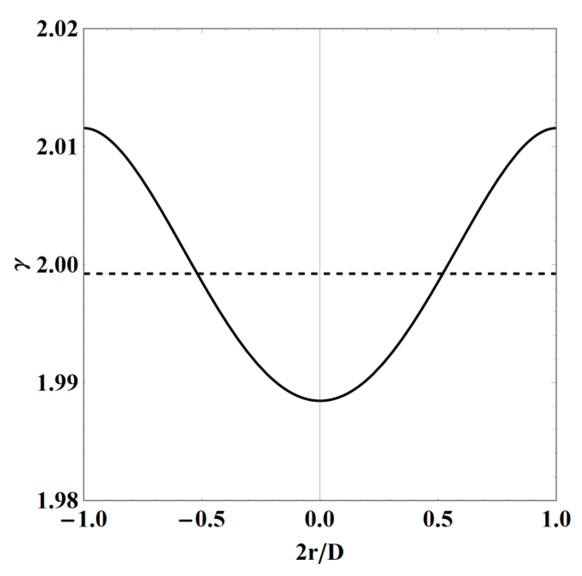
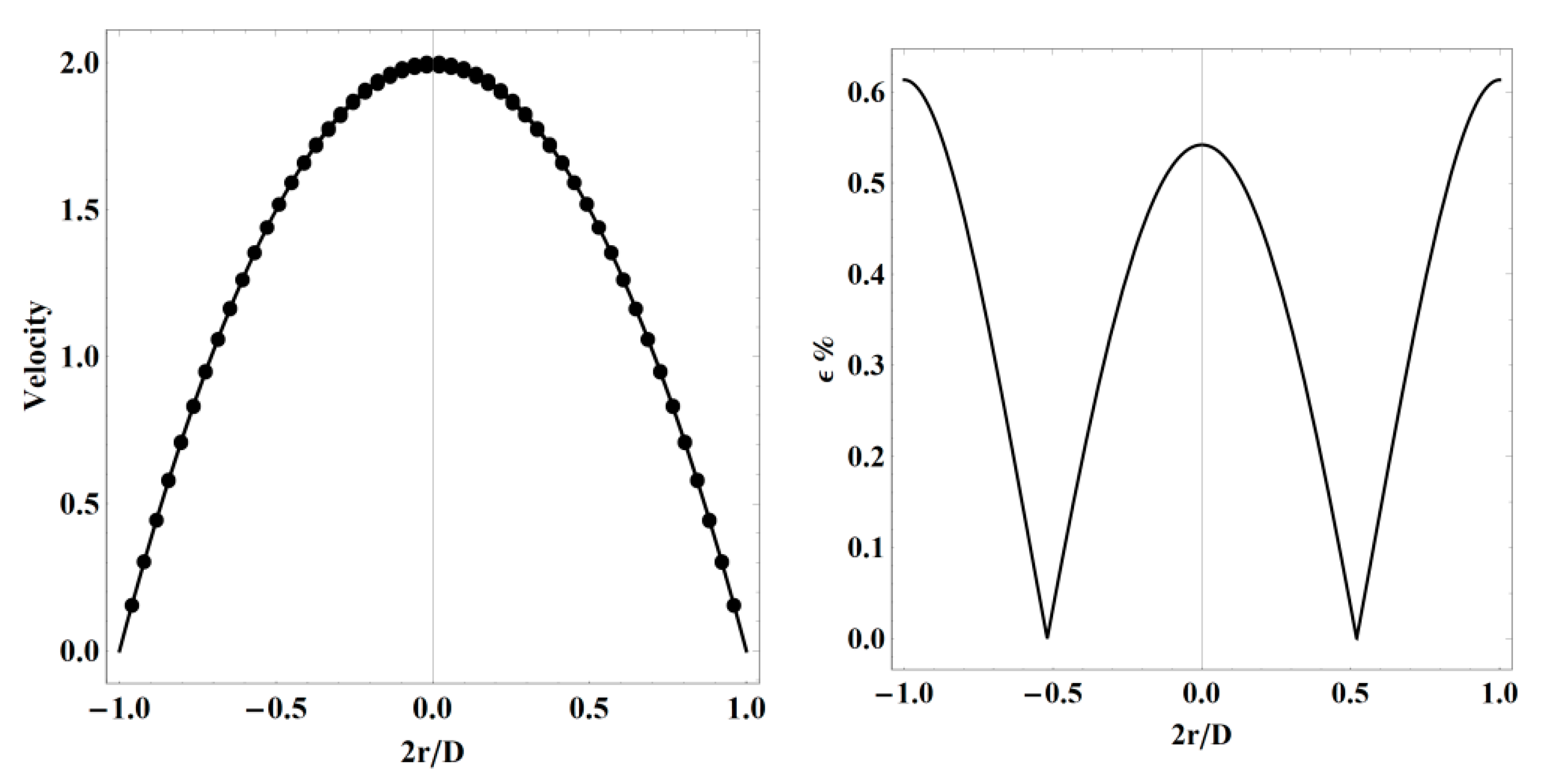
Figure 1. γ function (continuous line) and its average value 1.99923 (dashed line). Plot considering the example values: ρ = 1060 kg/m3, η = 3.45 × 10⁻³ Pa s, D = 0.003 m, T = 1.68 s and Wo = 1.61.
Dynamics 01 00002 g001
Figure 2. Comparison between the Womersley profile (line) and the transient Poiseuille profile (dot). Non-dimensional velocity comparison (left); percentage error (right). Plot considering the example values: ρ = 1060 kg/m3, η = 3.45 × 10⁻³ Pa s, D = 0.003 m, T = 1.68 s and Wo = 1.61.
Dynamics 01 00002 g002
Figure 3. Different shape of the Womersley function due to the different Womersley number varies.
Dynamics 01 00002 g003
Figure 4. Computational domain and Mesh.
Dynamics 01 00002 g004
Figure 5. Comparison between the original Womersley profile (line) and the transient Poiseuille function profile (dot) using several times in different sections. The velocity was considered in m/s.
Dynamics 01 00002 g005
Table 1. Numerical value of the Womersley f(2r/D) profile and Poiseuille profile considering the example values: ρ = 1060 kg/m3, η = 3.45 × 10⁻³ Pa s, D = 0.003 m, T = 1.68 s, and Wo = 1.61.
2r/Df(2r/D)vP(2r/D)ε%2r/Df(2r/D)vP(2r/D)ε%
0.001.988451.999230.5420610.551.395211.394460.053681
0.051.983601.994230.5362410.601.281331.279510.142441
0.101.969021.979240.5188700.651.157221.154560.230149
0.151.944721.954250.4902210.701.022831.019610.314656
0.201.910651.919260.4507450.750.878120.874660.393649
0.251.866791.874280.4010730.800.723080.719720.464652
0.301.813101.819300.3420120.850.557720.554790.525025
0.351.749521.754330.2745470.900.382040.379850.571956
0.401.676011.679360.1998340.950.196110.194930.602458
0.451.592491.594390.1192001.000.000000.00000-
0.501.498911.499420.034141
Publisher’s Note: MDPI stays neutral with regard to jurisdictional claims in published maps and institutional affiliations.

