Article

Intercept Capacity: Unknown Unitary Transformation

1
Department of Electrical and Electronic Engineering, University of Melbourne, Australia
2
EWRD, DSTO, PO Box 1500, Edinburgh, Australia
*
Author to whom correspondence should be addressed.
Submission received: 22 May 2008 / Accepted: 10 November 2008 / Published: 20 November 2008

Abstract

:
We consider the problem of intercepting communications signals between Multiple-Input Multiple-Output (MIMO) communication systems. To correctly detect a transmitted message it is necessary to know the gain matrix that represents the channel between the transmitter and the receiver. However, even if the receiver has knowledge of the message symbol set, it may not be possible to estimate the channel matrix. Blind Source Separation (BSS) techniques, such as Independent Component Analysis (ICA) can go some way to extracting independent signals from individual transmission antennae but these may have been preprocessed in a manner unknown to the receiver. In this paper we consider the situation where a communications interception system has prior knowledge of the message symbol set, the channel matrix between the transmission system and the interception system and is able to resolve the transmissionss from independent antennae. The question then becomes: what is the mutual information available to the interceptor when an unknown unitary transformation matrix is employed by the transmitter.

1. Introduction

In this paper we are interested in differential entropy and mutual information as it applies to wireless communication systems employing antenna arrays at both the transmission and receiving sites. Systems of this type are more commonly known as Multiple-Input Multiple-Output (MIMO) communication systems. MIMO communication techniques are known to provide increased information capacity over that
Figure 1. MIMO Wireless Intercept Model.
Entropy 10 00722 g001
Figure 2. 
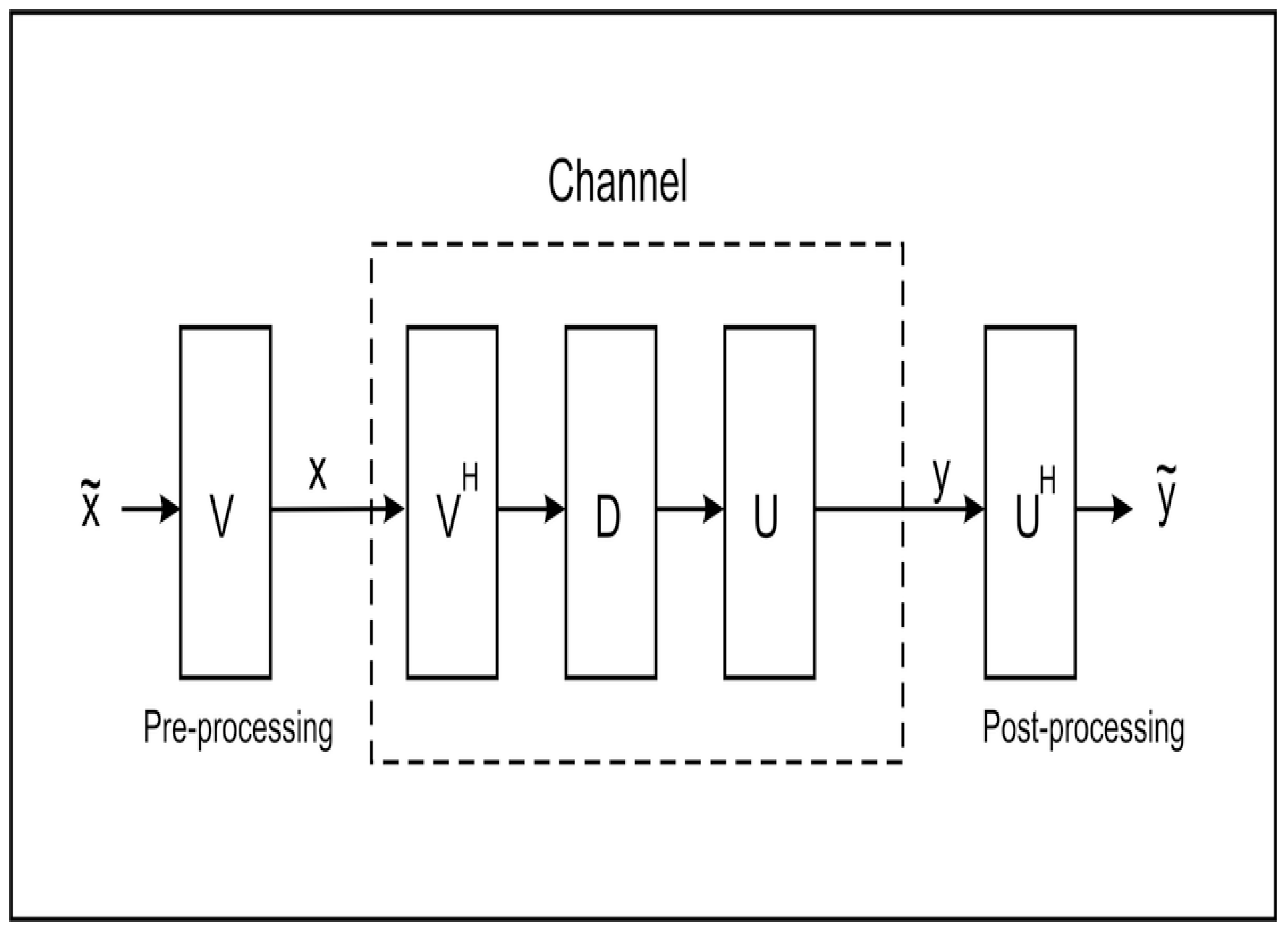
Converting MIMO channel to parallel channel via SVD.
Entropy 10 00722 g002
obtainable via a single transmit antenna to single receive antenna system [1, 2]; however this extra capacity comes at the expense of increased system complexity and additional processing. To correctly receive and detect the transmitted message, the receive system must know the channel, or mixing, matrix as well as the message symbol set being used. The channel matrix may be estimated when a predetermined, known message sequence is incorporated into the transmitted message and the receiver knows where in the message this sequence occurs. However this training sequence may not always be available and this presents a blind source estimation problem where neither the message nor the channel matrix are known to the receiver. One possible solution to this problem is to employ a Blind Source Separation (BSS) technique such as Independent Component Analysis (ICA) [3] which can go some way to extracting the signals from individual transmission antennae with the caveat that all but one of the transmitted signals must have a non-gaussian probability distribution. In some cases the transmitted signals may have been preprocessed in a manner unknown to the receiver. In this paper we consider the situation where a communications receiving system has prior knowledge of the message symbol set, the channel matrix between the transmission system and the receiving system, is able to resolve the transmissions from the, assumed independent, transmitter antennae but does not know the unitary transformation that has been applied at the transmitter. The question then becomes: what is the mutual information available to the receiver when an unknown unitary transformation matrix is employed by the transmitter?
In the following sections we derive expressions for differential entropy, mutual information and hence capacity for a two-element transmit array to two-element receive array system which we shall refer to as a 2-Dimensional (2D) system. The 3D case is studied in the appendix giving a basis for a high snr approximation for the general N-Dimensional (ND) case. The general snr, ND case is derived and the resulting intended-receiver and intercept receiver mutual informations are compared.

2. Problem and Assumptions

The model that we shall employ for a MIMO system is the simple linear transformation
y = H x + n
where y is the received signal vector, x is the transmitted vector, n is additive receiver noise and H is the channel gain or mixing matrix between the transmitter and receiver. The standard MIMO channel model [11] assumes independent identically distributed (i.i.d.), frequency-flat Rayleigh fading between the transmit and receive antennae. Consequently the components H i , j of H are typically modelled with a complex Normal density i.e. H i , j C N ( 0 , 1 ) . Here we shall assume H to be constant for both the intended and eavesdropper channels. In [11] the authors show that, for the case where the channel is unknown and with block coding over a coherence time T, the signal structure that achieves capacity is formed by the product of an isotropically distributed unitary matrix and a independent real, nonnegative diagonal matrix. For the purpose of this study we shall treat all of y , x , and n as real random variables. The benefit of this approach will be to simplify the derivations whilst recognising that, if the real and imaginary parts of the variables are independent, the results may be readily extended to the complex case by increasing the dimensionality of the vectors.
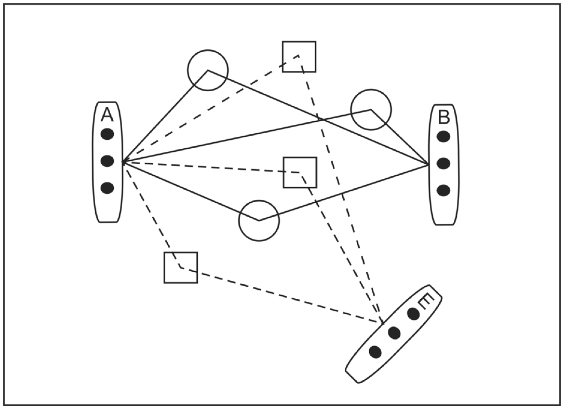
Figure 1 illustrates the scenario that we are studying. Employing a well-known cryptographic convention [4], the transmission source array is labelled Alice (A), the intended cooperative receiver array is labelled Bob (B) and the unintended, passive intercept receiver is labelled Eve (E). The lines represent the paths that signals take from transmitter antennae to receiver antennae. Shapes in the signal paths represent objects that cause signal scattering. An important point to realise here is that the paths (channel H B ) between A and B are different to those between A and E (channel H E ).
The channel matrix can be factorized using Singular Value Decomposition (SVD) as : H = UDV and we can then use:
U y = DV x + U n or y ˜ = D x ˜ + n ˜ .
This allows us to view the MIMO system as if it were composed of a set of parallel channels and the input data vector can be designed with this in mind. Figure 2 shows how this channel, with pre and post-processing, may be configured. For such an approach to work the transmitter requires precise knowledge of the channel matrix and it is a simple matter for the intended receiver to obtain the (scaled) message, since D is a real diagonal matrix. However for an unintended receiver, with a different (known) channel matrix, an unknown unitary transformation has been applied. In this case we desire to know how the mutual information, is affected. We make the following assumptions:
  • y is a real N × 1 observation vector.
  • U is a real N × N unitary (orthogonal) matrix.
  • x is a real N × 1 random Gaussian signal vector, x i N ( 0 , σ x 2 ) .
  • n is a real N × 1 random Gaussian noise vector, n i N ( 0 , σ n 2 ) .
  • | | x | | = i = 1 N x i 2 = A = constant .
  • the intended channel ( H B ) is known to both Alice and Bob.
  • Eve knows the intercept channel ( H E ) but not the intended channel.
  • the channels H B and H E vary slowly with time (or over many symbol periods) and may be assumed constant for the present study.
Based on the last assumption, Eve attempts to estimate the signal vector by applying the channel inverse as
x ^ = H E 1 y = V x ˜ + H E 1 n E .
Eve is therefore unable to directly obtain x ˜ due to the unknown unitary matrix V . In applying the channel inverse, the noise vector has also been scaled and the modified noise covariance term H e 1 Σ n H e T shows that the intercept receiver may be operating with a different signal to noise ratio to that of the intended receiver. This also indicates that Eve could obtain better mutual information with a better channel.
Optimal power allocation to the parallel channels between Alice and Bob would typically be implemented via a technique called waterfilling, see [5] chapter 5, and hence lead to optimal system capacity. We have not taken waterfilling into account in this study and simply assume that equal power is assigned to each of the parallel channels.
We could proceed to derive the eavesdropper mutual information in a cartesian or a polar coordinate system. Of course it doesn’t matter which coordinate system we choose - we should get the same answer. It is well known that differential entropy involves a Jacobian (J) in the transformation of coordinates [6] , leading to a ln det ( J ) term but this will cancel in the mutual information calculations because mutual information is a relative entropy i.e. the difference between two entropies. For the purpose of this study our derivations will be based on a cartesian coordinate system. We shall derive differential entropies according to the definitions given by Cover and Thomas in [7], i.e. the differential entropy h ( Y ) of a continuous random variable Y with a probability density p ( y ) is defined as
h ( Y ) Y p ( y ) ln ( p ( y ) ) d y ,
where Y is the support set of the random variable. When we have two random variables Y , X with joint probability density p ( y , x ) , the conditional differential entropy is defined as
h ( Y | X ) Y , X p ( y , x ) ln ( p ( y | x ) ) d y d x ,
where X is the support set of the random variable X. The Mutual Information (MI) between the two random variables Y and X is defined as
I ( Y ; X ) = Y , X p ( y , x ) ln p ( y , x ) p ( y ) p ( x ) d y d x = h ( Y ) h ( Y | X ) = h ( X ) h ( X | Y ) .
The capacity C is then obtained by maximizing the mutual information over all probability distributions for the source i.e. over p ( x ) :
C = sup p ( x ) I ( Y ; X ) .
It is well known [7] that a Gaussian source distribution is an entropy maximizer (for a given variance) so that, by treating x as a vector with i.i.d Gaussian components, the resulting differential entropy expressions will determine the capacity. Since the channels are assumed known we may consider
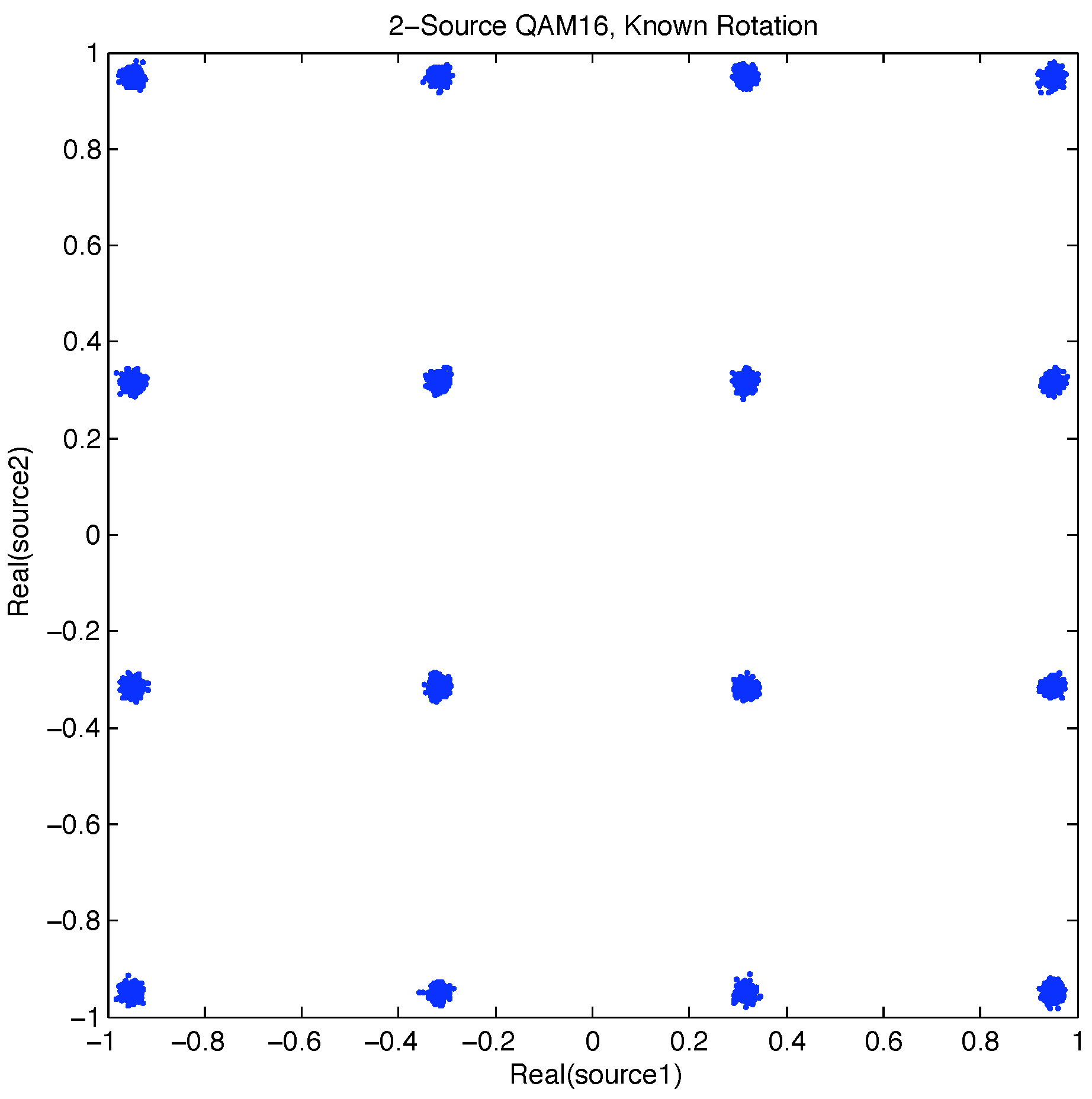
 y = x + n
Figure 3. 2D Transmitter message symbol set.
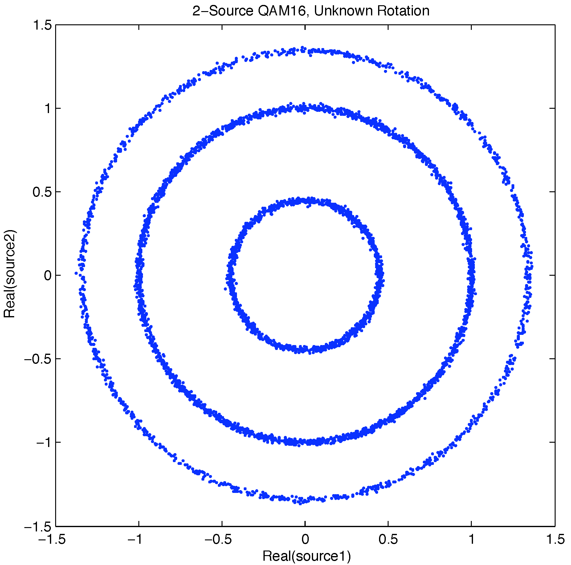
Entropy 10 00722 g003
Figure 4. Received ring distribution caused by unknown rotation on message symbol set.
Entropy 10 00722 g004
to represent the fully informed (unitary transformation known) case and y = Vx + n to represent the partially informed (unitary transformation unknown) case. We can write x = x | | x | | | | x | | to obtain
y = V x | | x | | | | x | | + n = v A + n
where A = | | x | | and v = V x | | x | | is a unit vector for which we may or may not know the rotations. For the random vectors y and x the mutual information for the fully informed model is given by:
I F = h ( y ) h ( y | x , V )
and for the partially informed model the mutual information is obtained from:
I P = h ( y ) h ( y | A )
where the message amplitude A is known but not the rotation angles.

3. 2D Capacity

To illustrate the consequence of not knowing the rotation imposed by the orthogonal transformation in the 2D case, figure 3 shows a message symbol set where each of the two transmitters can set one of four possible values. Thus a constellation containing 16 points may be realised at the receiver and the density of these points is determined by the additive noise. If the rotation is unknown but the amplitude levels are known then the receiver might obtain a message that looks something like figure 4 where the density of the rings is determined by the additive noise.

3.1. 2D Density Function

We can construct the joint density function beginning with
p ( y 1 , y 2 | x 1 , x 2 ) = p ( y 1 | x 1 ) p ( y 2 | x 2 ) = 1 2 π σ n 2 exp [ y x ] T [ y x ] 2 σ n 2
and then letting | x | 2 = x 1 2 + x 2 2 , x 1 = | x | cos α and x 2 = | x | sin α i.e. | x | is the magnitude of the vector [ x 1 x 2 ] T and α is the angle of this vector relative to the origin. Similarly | y | 2 = y 1 2 + y 2 2 , y 1 = | y | cos ϕ and y 2 = | y | sin ϕ , where | y | is the magnitude of the vector [ y 1 y 2 ] T and ϕ is the angle of this vector relative to the origin.
so that
p ( y 1 , y 2 | x 1 , x 2 ) = 1 2 π σ n 2 exp | y | 2 | x | 2 2 | x | | y | cos ( ϕ α ) 2 σ n 2 .

3.2. x and V known

In this case V rotates the original vector x o through a known angle to a new, known x and we can treat this case with the probability density function (pdf)
p ( y 1 , y 2 | x 1 , x 2 ) = 1 ( 2 π σ n 2 ) exp ( y 1 x 1 ) 2 2 σ n 2 1 ( 2 π σ n 2 ) exp ( y 2 x 2 ) 2 2 σ n 2
and the differential entropy is
h ( y | x ) = 0 p ( y | x ) ln p ( y | x ) d y = 1 2 ln ( 2 π e σ n 2 ) + 1 2 ln ( 2 π e σ n 2 ) = ln ( 2 π e σ n 2 ) .

3.3. A known, V unknown

In this case V rotates the original vector x o through an unknown angle γ so that x 1 = A cos γ and x 2 = A sin γ , giving the pdf
p ( y 1 , y 2 | A , γ ) = 1 ( 2 π σ n 2 ) exp | y | 2 A 2 2 σ n 2 exp A | y | cos ( ϕ γ ) σ n 2 .
Now, with β ϕ γ and p ( β ) = 1 2 π ,
p ( y 1 , y 2 | A ) = 0 2 π p ( y 1 , y 2 | A , β ) p ( β ) d β = 1 2 π σ n 2 exp | y | 2 A 2 2 σ n 2 I 0 A | y | σ n 2 .
At high enough SNR we may approximate the Bessel function as
I 0 ( K x ) 1 K x exp { K x } .
Therefore
p ( y 1 , y 2 | A ) σ n 2 π σ n 2 ( 2 π A | y | ) exp ( | y | A ) 2 2 σ n 2 1 2 π A 1 2 π σ n 2 exp ( | y | A ) 2 2 σ n 2 .
and the differential entropy is
h ( y | A ) = 0 p ( y | A ) ln p ( y | A ) d y ln ( 2 π A ) + 1 2 ln ( 2 π e σ n 2 )

3.4. x and V unknown

In this case we assume that we only have knowledge of the variance of x and n and hence the variance of y . With the components of both x and n treated as zero-mean Gaussian, then the components of y will also be zero-mean Gaussian with variance equal to the sum of the variances of x and n i.e. y i N ( 0 , σ y 2 ) where σ y 2 = σ x 2 + σ n 2 . The joint pdf for y is
p ( y 1 , y 2 ) = 1 2 π σ y 2 exp y 1 2 2 σ y 2 1 2 π σ y 2 exp y 2 2 2 σ y 2
which leads us to the differential entropy
h ( y ) = 0 p ( y ) ln p ( y ) d y = 1 2 ln ( 2 π e σ y 2 ) + 1 2 ln ( 2 π e σ y 2 ) = ln ( 2 π e σ y 2 ) .

3.5. Capacity

The fully informed mutual information was defined in equation (8) and so when both x and V are given, with Gaussian distributions for the source and noise, we have the fully informed capacity
C F 2 = ln ( 2 π e σ y 2 ) ln ( 2 π e σ n 2 ) = ln σ y 2 σ n 2 .
Similarly partially informed mutual information was defined in equation (9) so that, when the rotation matrix is unknown, we obtain the partially informed capacity
C P 2 ln ( 2 π e σ y 2 ) ln ( 2 π A ) 1 2 ln ( 2 π e σ n 2 ) = ln σ y 2 A σ n + 1 2 ln e 2 π
In a similar fashion we may derive the entropies and mutual information for the 3D case. The derivation is given in Appendix A, where we find that
C F 3 = ln σ y 3 σ n 3 .
and
C P 3 ln σ y 3 A 2 σ n + ln e 2

4. ND Capacity

4.1. High SNR Case

At high snr we found that the partially informed probability density functions factored into two parts:
2D case: p ( y | A ) 1 2 π A 1 2 π σ n 2 exp ( | y | A ) 2 2 σ n 2 3D case: p ( y | A ) 1 4 π A 2 1 2 π σ n 2 exp ( | y | A ) 2 2 σ n 2 .
The first part appears to have the form of a uniform density on the surface of an N-dimensional sphere. The second part appears to represent a Gaussian distribution across an N-dimensional shell. Therefore p ( y | A ) may be viewed as an N-dimensional, variable density, shell with mean radius A. From Wikipedia (“Sphere”) [8] the general equations for the surface area and volume of an N-dimensional sphere, with radius A = i N x i 2 , are given by:
Surface Area = 2 π N 2 A N 1 Γ N 2
and
Volume = 2 π N 2 A N N Γ N 2
Thus the required N-D, high SNR entropies, may be written as:
h ( y | x ) = N 2 ln ( 2 π e σ n 2 ) ,
h ( y | A ) ln 2 π N 2 A N 1 Γ N 2 + 1 2 ln 2 π e σ n 2 ,
h ( y ) = N 2 ln ( 2 π e σ y 2 ) .
The densities p ( y ) and p ( y | x ) could be pictured as N-dimensional, probability spheres. Hence the fully informed capacity becomes the difference in entropy between an N-dimensional probability sphere, representing the signal plus noise vector distribution, and an N-dimensional sphere, representing the noise vector distribution. In the partially informed case the capacity becomes the difference in entropy between an N-dimensional probability sphere, representing the signal plus noise vector distribution, and an N-dimensional probability shell, representing the amplitude known plus noise distribution. The ND fully informed capacity may be written as
C F N = h ( y ) h ( y | x ) = N 2 ln σ y 2 σ n 2
and the partially informed capacity may be approximated by
C P N h ( y ) h ( y | A ) = 1 2 ln σ y 2 σ n 2 + 1 2 ln π 1 2 N 3 e N 1 + ln Γ N 2 .
Defining the signal-to-noise ratio as ρ = A 2 σ n 2 and with σ y 2 = σ x 2 + σ n 2 = A 2 + σ x 2 , then the capacities may be expressed as
C F N N 2 ln 1 + ρ
C P N 1 2 ln 1 + ρ + 1 2 ln π 1 2 N 3 e N 1 + ln Γ N 2 .

4.2. General Case

In this section we derive the general form for p ( y | A ) thus allowing us to obtain the capacity for any dimension and snr. The derivation utilises a result by Vesely [9] that shows how the “mass” of an N dimensional spherical shell is distributed along one sphere axis. This result greatly simplifies the multidimensional integrals that we require to solve. The surface area, S N ( r 0 ) , of an N dimensional sphere, as a function of radius, may be represented as
S N ( r 0 ) = r 0 r 0 r 0 S N 1 ( r 2 ) r 2 d r 1
where r 2 = r 0 2 r 1 2 . We can rewrite the above as
1 = r 0 r 0 r 0 S N 1 ( r 2 ) r 2 S N ( r 0 ) d r 1 = r 0 r 0 p N ( r 1 ) d r 1
which shows how the “mass”of the shell is distributed along the single sphere axis r 1 .
p N ( r 1 ) = r 0 S N 1 ( r 2 ) r 2 S N ( r 0 ) = ( N 1 ) C N 1 r 2 N 3 N C N r 0 N 2 = ( N 1 ) C N 1 N C N 1 r 0 1 r 1 2 r 0 2 N 3 2
where
C N = 2 π N / 2 N Γ ( N / 2 ) .
The integrals that we are dealing with take the form
p ( y | x ) = ( 2 π σ n 2 ) N / 2 exp | y | 2 | x | 2 2 σ n 2 exp i = 1 N x i y i σ n 2 = ( 2 π σ n 2 ) N / 2 exp | y | 2 | x | 2 2 σ n 2 exp x y σ n 2
from which we wish to obtain p ( y | | x | ) . Assuming now that | x | is given we have
p ( y | x , | x | ) = ( 2 π σ n 2 ) N / 2 exp | y | 2 | x | 2 2 σ n 2 exp x y σ n 2
and so to obtain p ( y | | x | ) we must integrate over the x i as follows
p ( y | | x | ) = | x | = A p ( y | x , | x | ) p ( x ) d x = ( 2 π σ n 2 ) N / 2 exp | y | 2 | x | 2 2 σ n 2 | x | = A exp x y σ n 2 p ( x ) d x
We proceed to calculate this integral by first noting that the x i are uniformly distributed over the surface of an N-dimensional sphere and we only need to perform the integral along a single dimension, e.g. x 1 and replace p ( x ) with p ( x 1 ) using the results derived earlier. To better understand this, consider the dot product x y . The dot product will be unchanged if both vectors are operated on by the same rotation matrix. Let the rotation matrix be M R N × N , then
( M x ) ( M y ) = ( M x ) T ( M y ) = x T M T M y = x T y = x y
since M M T = M M 1 = I . So we are free to choose any rotation matrix and the integral will be unaffected. Let us choose M such that M y = | y | [ 1 , 0 , , 0 ] = | y | e , where e is a unit vector, i.e. the vector y is rotated to lie along the y 1 axis. Let x = ( M x ) then we have
x ( M y ) = x | y | e = | y | ( x ) T e = | y | x 1 .
Hence, with | x | = A ,
| x | = A exp x y σ n 2 p ( x ) d x = A A p N ( x 1 ) exp | y | x 1 σ n 2 = ( N 1 ) C N 1 N C N 1 A A A 1 x 1 2 A 2 N 3 2 exp | y | x 1 σ n 2 d x 1
We may make a change of variable by letting z = x 1 A to get
| x | = A exp x y σ n 2 p ( x ) d x = ( N 1 ) C N 1 N C N 1 1 1 z 2 N 3 2 exp | y | A z σ n 2 d z
The general form for the density, given A, is therefore
p ( y | A ) = ( 2 π σ n 2 ) N 2 exp A 2 | y | 2 2 σ n 2 ( N 1 ) C N 1 N C N 1 1 1 z 2 N 3 2 exp | y | A z σ n 2 d z .
The entropy calculation involves a multidimensional integration over the components in y :
h ( y | A ) = y p ( y | A ) ln p ( y | A ) d y .
With the general form for the differential entropies we are now able to derive the capacity for both the fully informed cases and the partially informed (amplitude only) cases. The capacity for dimensions two to five have been calculated for both cases and the results are presented in figure 5 and figure 6. Comparing the two figures we note that the partially informed curves have a smaller slope than their fully informed counterparts. If both receivers were operating with the same snr then we could also make the observation that the partially informed values are always less than their fully informed counterparts. However, as indicated in section 2 earlier, due to the channel matrix inversion required by Eve and a possibly different local (local to the receivers) noise environment, this may not be the case.

5. Summary

The problem of determining the information intercept capacity, available to a receiving system which knows its channel matrix but has no prior knowledge of a unitary transformation that has been applied at the transmitter, has been analysed. Entropy derivations were carried out for two dimensions and three dimensions giving some insight to the general dimensional, high snr case. The exact capacity for the N-Dimensional case has been obtained but requires numerical integration to derive the differential entropy for the partially informed case.
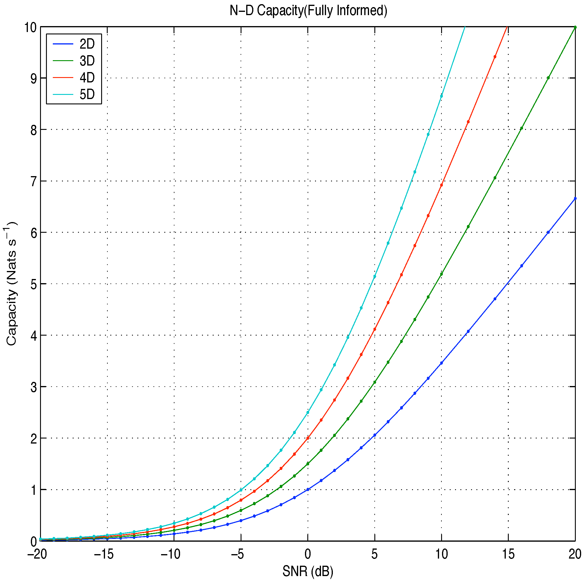
Figure 5. Capacity: fully informed Vs SNR.
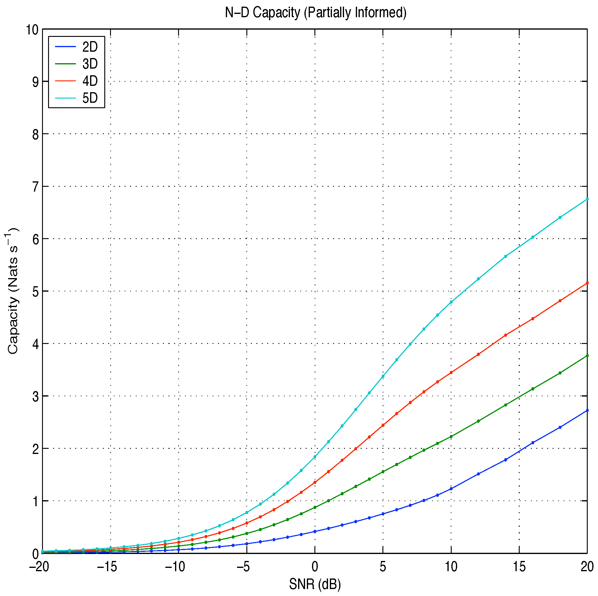
Entropy 10 00722 g005
Figure 6. Capacity: partially informed Vs SNR.
Entropy 10 00722 g006
The fully informed capacity has been likened to the difference in entropy between two N-dimensional probability spheres: the larger sphere, representing the distribution of the signal plus noise vector, and the smaller sphere, representing the distribution of the noise vector. At high snr, the partially informed capacity was found to be equal to the difference in entropy between an N-dimensional probability sphere, representing the distribution of the signal plus noise vector, and an N-dimensional probability shell, representing the distribution of the amplitude plus noise vector.

Acknowledgements

We would like to thank the anonymous reviewers for their observations and helpful suggestions, which improved the original manuscript.

References and Notes

  1. Foschini, G.J.; Gans, M.J. On Limits of Wireless Communications in a Fading Environment when Using Multiple Antennas. Wireless Pers. Commun. 1998, 6, 311–335. [Google Scholar]
  2. Telatar, E. Capacity of Multi-antenna Gaussian Channels, AT&T-Bell Lab. Internal Tech. Memo. 1995. [Google Scholar]
  3. Comon, P. Independent Component Analysis, A new concept? Signal Process. 1994, 36, 287–314. [Google Scholar] [CrossRef] [Green Version]
  4. Maurer, U.M. Secret Key Agreement by Public Discussion From Common Information. IEEE Trans. Inform. Theory 1993, 39, 733–742. [Google Scholar] [CrossRef]
  5. Tse, D.; Viswanath, P. Fundamentals of Wireless Communication; Cambridge University Press: U.K, 2005. [Google Scholar]
  6. Papoulis, A. Probability, Random Varables, and Stochastic Processes; McGraw-Hill, 1989. [Google Scholar]
  7. Cover, T.M.; Thomas, J.A. Elements of Information Theory; John Wiley & Sons, Inc., 1991. [Google Scholar]
  8. Wikipedia. N-sphere — Wikipedia, The Free Encyclopedia. 2008. http://en.wikipedia.org/wiki/N-sphere.
  9. Vesely, F. From Hyperspheres to Entropy. http://homepage.univie.ac.at/franz.vesely/sp.english/sp/sp.html.
  10. Prudnikov, A.P.; Brychkov, Yu.A.; Marichev, O.I. Integrals and Series; Gordon and Breach Sci. Publ.: New York, 1986; p. 464. [Google Scholar]
  11. Marzetta, T.L.; Hochwald, B.M. Capacity of a Mobile Multiple-Antenna Communication Link in Rayleigh Flat Fading. IEEE Trans. Inform. Theory 1999, 45, 139–157. [Google Scholar] [CrossRef]

Appendix: Derivation of 3D Mutual Information

We can construct the joint probability density function in the following manner. Beginning with
p ( y 1 , y 2 , y 3 | x 1 , x 2 , x 3 , V ) = 1 ( 2 π σ n 2 ) 3 2 exp [ y Vx ] T [ y Vx ] 2 σ n 2

x known

In the case where x is known after the transformation the pdf is given by
p ( y 1 , y 2 , y 3 | x 1 , x 2 , x 3 ) = exp ( y 1 x 1 ) 2 2 σ n 2 ( 2 π σ n 2 ) exp ( y 2 x 2 ) 2 2 σ n 2 ( 2 π σ n 2 ) exp ( y 3 x 3 ) 2 2 σ n 2 ( 2 π σ n 2 )
and the entropy is
h ( y | x ) = 0 p ( y | x ) ln p ( y | x ) d y = 1 2 ln ( 2 π e σ n 2 ) + 1 2 ln ( 2 π e σ n 2 ) + 1 2 ln ( 2 π e σ n 2 ) = 3 2 ln ( 2 π e σ n 2 ) .

A known, α , β unknown

For the vector [ x 1 x 2 x 3 ] T there are two rotation angles to consider: α , β and so, with
| x | 2 = A 2 x 1 = A sin α cos β x 2 = A sin α sin β x 3 = A cos α ,
we have the joint probability of the two angles p ( α , β ) = sin α 4 π . Therefore p ( y | x ) p ( y | A , α , β ) becomes
p ( y | x ) = 1 ( 2 π σ n 2 ) 3 2 exp | y | 2 | x | 2 2 σ n 2 exp x 1 y 1 + x 2 y 2 + x 3 y 3 σ n 2 p ( y | A , α , β ) = 1 ( 2 π σ n 2 ) 3 2 exp | y | 2 A 2 2 σ n 2 exp A σ n 2 [ sin α cos β y 1 + sin α sin β y 2 + cos α y 3 ]
The integral
p ( y | A ) = 0 2 π 0 π p ( y | A , α , β ) p ( α , β ) d α d β
is obtained by using the form given in Prudnikov et al [10] :
0 2 π 0 π sin α exp A σ n 2 [ sin α cos β y 1 + sin α sin β y 2 + cos α y 3 ] d α d β = 2 π σ n 2 A | y | exp A | y | σ 2
and so
p ( y | A ) = 1 4 π A | y | 1 2 π σ n 2 exp ( | y | A ) 2 2 σ n 2 ,
which may be approximated, at high SNR, as:
p ( y | A ) 1 4 π A 2 1 2 π σ n 2 exp ( | y | A ) 2 2 σ n 2 ,
The differential entropy is
h ( y | A ) = 0 p ( y | A ) ln p ( y | A ) d y ln ( 4 π A 2 ) + 1 2 ln ( 2 π e σ n 2 )

x unknown

In this case we assume that we only have knowledge of the variance of x and n and hence the variance of y . With both x and n treated as zero-mean Gaussian, then y will also be zero-mean Gaussian with variance equal to the sum of the variances of x and n i.e. y i N ( 0 , σ y 2 ) where σ y 2 = σ x 2 + σ n 2 .
p ( y 1 , y 2 , y 3 ) = exp y 1 2 2 σ y 2 2 π σ y 2 exp y 2 2 2 σ y 2 2 π σ y 2 exp y 3 2 2 σ y 2 2 π σ y 2
giving the differential entropy as
h ( y ) = 0 p ( y ) ln p ( y ) d y = 1 2 ln ( 2 π e σ y 2 ) + 1 2 ln ( 2 π e σ y 2 ) + 1 2 ln ( 2 π e σ y 2 ) = 3 2 ln ( 2 π e σ y 2 ) .

Capacity

Define I F h ( y ) h ( y | x )
and I P h ( y ) h ( y | A )
where I F is the mutual information in the best case where both x and V are given. I P is the mutual information when the rotation matrix is unknown. Since the source and noise distributions are Gaussian, and assuming constant source variance, we then obtain the fully informed and partially informed capacities as
C F 3 = 3 2 ln ( 2 π e σ y 2 ) 3 2 ln ( 2 π e σ n 2 ) = ln σ y 3 σ n 3
and
C P 3 = 3 2 ln ( 2 π e σ y 2 ) ln ( 4 π A 2 ) 1 2 ln ( 2 π e σ n 2 ) = ln σ y 3 A 2 σ n + ln e 2

