An Assessment of Hermite Function Based Approximations of Mutual Information Applied to Independent Component Analysis

Abstract
:1. Introduction
2. Independent Component Analysis and Mutual Information
2.1. Orthogonal Series for Nonparametric Density Estimation
2.2. Kernel Density Estimation
2.3. RADICAL

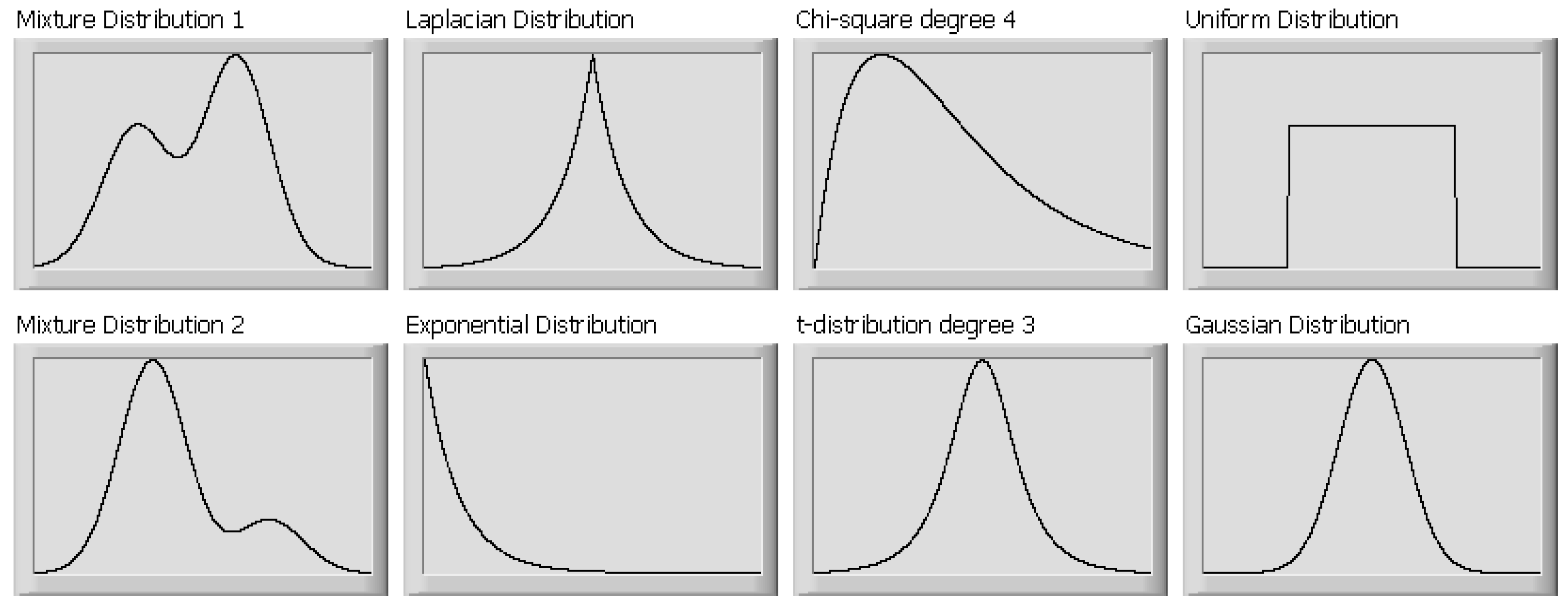
| Distribution 1 | Distribution 2 | |
| Scenario 1 | , | |
| Scenario 2 | Laplacian | Gaussian |
| Scenario 3 | t-distribution, degree 3 | t-distribution, degree 5 |
| Scenario 4 | Exponential distribution | t-distribution, degree 3 |
| Scenario 5 | Exponential distribution | Uniform |
| Scenario 6 | Chi-squared, degree 3 | Uniform |
| Scenario 7 | Gaussian | Uniform |
| Scenario 8 | Gaussian | t-distribution, degree 4 |
2.4. FastICA
3. Simulations

| Shannon MI: Hermite | Renyi MI: Hermite | Shannon MI: Kernel | Renyi MI: Kernel | RADICAL | FastICA | |
| Scenario 1 | 3.0 | 2.9 | 2.3 | 2.8 | 2.7 | 2.4 |
| Scenario 2 | 5.9 | 4.0 | 3.9 | 3.7 | 5.1 | 3.1 |
| Scenario 3 | 2.5 | 1.5 | 1.6 | 1.6 | 1.5 | 2.1 |
| Scenario 4 | 1.9 | 1.3 | 1.4 | 1.4 | 1.3 | 2.2 |
| Scenario 5 | 1.4 | 1.6 | 1.4 | 1.7 | 1.4 | 2.8 |
| Scenario 6 | 1.6 | 2.0 | 1.6 | 2.2 | 1.6 | 2.7 |
| Scenario 7 | 2.4 | 3.3 | 2.3 | 3.6 | 2.3 | 4.2 |
| Scenario 8 | 4.9 | 1.8 | 2.1 | 2.2 | 1.7 | 2.2 |
| mean | 3.0 | 2.3 | 2.1 | 2.4 | 2.2 | 2.7 |

| Shannon MI: Hermite | Renyi MI: Hermite | Shannon MI: Kernel | Renyi MI: Kernel | RADICAL | FastICA | |
| 1000 points | 3 | 1 | 244 | 244 | 54 | 0 |
| 2000 points | 5 | 2 | 485 | 485 | 110 | 0 |
| 4000 points | 9 | 5 | 3786 | 3786 | 238 | 1 |
| 8000 points | 21 | 10 | 14978 | 14978 | 485 | 2 |
4. Further Work
5. Conclusion
Acknowledgements
References and Notes
- Amari, S.; Cichocki, A.; Yang, H. H. A new learning algorithm for blind signal separation. Advances in Neural Information Processing Systems 1996, 8, 757–763. [Google Scholar]
- Bingham, E.; Hyvarinen, A. A fast fixed-point algorithm for independent component analysis of complex-valued signals. Int. J. of Neural Syst. 2000, 10 (1), 1–8. [Google Scholar] [CrossRef]
- Boscolo, R.; Pan, H.; Roychowdhury, V. P. Independent component analysis based on nonparametric density estimation. IEEE Trans. Neural Networks. 2004, 55–65. [Google Scholar] [CrossRef]
- Como, P. Independent component analysis, A new concept? Signal Process. 1994, 287–314. [Google Scholar] [CrossRef] [Green Version]
- Erdogmus, D.; Hild II, K. E.; Principe, J. C. Independent components analysis using Renyi’s mutual information and Legendre density estimation. In Proceedings of International Joint Conference on Neural Networks, USA, July 2001, 4; pp. 2762–2767.
- Hild II, K. E.; Erdogmus, D.; Principe, J. C. Blind source separation using Renyi’s mutual information. IEEE Signal Process. Lett. 2001, 8, 174–176. [Google Scholar] [CrossRef]
- Hyvarinen, A. Fast and robust fixed-point algorithms for independent component analysis. IEEE Trans. Neural Networks. 1999, 10, 626–634. [Google Scholar] [CrossRef] [PubMed]
- Hyvarinen, A.; Karhunen, J.; Oja, E. Independent Component Analysis. John Wiley & Sons, 2001. [Google Scholar]
- Izenman, A.J. Recent developments in nonparametric density estimation. J. Amer. Statistical Assoc. 1991, 86, 205–223. [Google Scholar] [CrossRef]
- Learned-Miller, E. G.; Fisher III, J. W. ICA using spacing estimates of Entropy. J. Mach. Learn. Res. 2003, 4, 1271–1295. [Google Scholar]
- Lee, I.; Lee, T. Nonparameteric Independent Component Analysis for Circular Complex Variables. In Proceedings of IEEE International Conference on Acoustics, Speech and Signal Processing, Honolulu, 2007, 2; pp. 665–668.
- Obradovic, D.; Deco, B. Information maximization and independent component analysis: Is there a difference? Neural Computat. 2000, 2085–2101. [Google Scholar] [CrossRef]
- Parzen, E. On esimation of a probability density function and mode. Ann. Math. Statist. 1962, 33, 1065–1076. [Google Scholar] [CrossRef]
- Silverman, B. W. Density Estimation for Statistics and Data Analysis, Chapman and Hall. 1985. [Google Scholar]
- Schwartz, S. C. Estimation of a probability density by an orthogonal series. Ann. Math. Statist. 1966, 38, 1262–1265. [Google Scholar] [CrossRef]
- Walter, G. G. Properties of Hermite series estimation of probability density. Ann. Statist. 1977, 5, 1258–1264. [Google Scholar] [CrossRef]
- Webb, A. Statistical Pattern Recognition; Hodder Arnold, 1999. [Google Scholar]
© 2008 by the authors; licensee Molecular Diversity Preservation International, Basel, Switzerland. This article is an open-access article distributed under the terms and conditions of the Creative Commons Attribution license (http://creativecommons.org/licenses/by/3.0/).
Share and Cite
Sorensen, J. An Assessment of Hermite Function Based Approximations of Mutual Information Applied to Independent Component Analysis. Entropy 2008, 10, 745-756. https://0-doi-org.brum.beds.ac.uk/10.3390/e10040745
Sorensen J. An Assessment of Hermite Function Based Approximations of Mutual Information Applied to Independent Component Analysis. Entropy. 2008; 10(4):745-756. https://0-doi-org.brum.beds.ac.uk/10.3390/e10040745
Chicago/Turabian StyleSorensen, Julian. 2008. "An Assessment of Hermite Function Based Approximations of Mutual Information Applied to Independent Component Analysis" Entropy 10, no. 4: 745-756. https://0-doi-org.brum.beds.ac.uk/10.3390/e10040745