Generalised Entropy of Curves for the Analysis and Classification of Dynamical Systems

Abstract

This paper provides a new approach for the analysis and eventually the classification of dynamical systems. The objective is pursued by extending the concept of the entropy of plane curves, first introduced within the theory of the thermodynamics of plane curves, to ${\mathbb{R}}^n$ space. Such a generalised entropy of a curve is used to evaluate curves that are obtained by connecting several points in the phase space. As the points change their coordinates according to the equations of a dynamical system, the entropy of the curve connecting them is used to infer the behaviour of the underlying dynamics. According to the proposed method all linear dynamical systems evolve at constant zero entropy, while higher asymptotic values characterise nonlinear systems. The approach proves to be particularly efficient when applied to chaotic systems, in which case it has common features with other classic approaches. Performances of the proposed method are tested over several benchmark problems.

1. Introduction

This paper provides a new approach for the analysis and eventually the classification of dynamical systems. Some classification methods are already known from literature and are now a cornerstone in modern systems theory. For instance, it is possible to classify a linear system as stable, asymptotically stable or unstable, on the basis of the eigenvalues of its transition matrix. The same approach can be extended to nonlinear systems applying a linearisation procedure with respect to some nominal evolution, although now information can only be inferred about the particular evolution. A less conventional method based on the time-frequency plane [1] is used to distinguish between 5 possible nonlinearities. This method can only be applied to SDOF (Single Degree Of Freedom) nonconservative systems, that is systems that can be described by (1)

$$\ddot{x}\left(t\right)+c\dot{x}\left(t\right)+f\left(x\left(t\right)\right)=0,$$

(1)

where c is a small positive parameter and $f\left(x\right)$ is a function of the state variable x identifying the type of nonlinearity. However, an extension of the previous approach to a wider class of nonlinearities still has to come. Alternatively, in [2], two systems are considered equivalent if any variable of one system may be expressed as a function of the variables of the other system and of a finite number of their derivatives. This is also known as Lie-Bäcklund isomorphism. From this point of view, the class of simplest systems, also called flat systems, includes all systems equivalent to a linear controllable system of any dimension with the same number of inputs. The drawback of this approach from a mathematical point of view is the difficulty of obtaining criteria for checking flatness. Besides, a complete classification of nonlinear systems according to the Lie-Bäcklund isomorphism is still to be done.

Chaotic systems are an important class of nonlinear systems. Chaotic attractors can be recognised by visual inspection of phase space portraits, and numerical quantification of chaos can be computed by several well known methods such as Lyapunov Exponents, auto-correlation functions and the power spectrum [3,4]. For instance, Lyapunov Exponents can be used to classify attractors into equilibria, cycles and chaotic sets. However, a drawback of this approach is that this classification makes sense only when the dynamical systems under exam admit attractive sets.

In this paper a novel method for comparing nonlinear systems is proposed and is based on a generalisation of the entropy of a plane curve [5]. Roughly speaking, the entropy of a curve is 0 when the curve is a straight line, and increases as the curve becomes more “wiggly". Starting from the seminal work of [5], a new theory, called “thermodynamics of curves", was developed [6], with some analogies with thermodynamics. However, defining the entropy of a curve only for plane curves has restricted its use to a few applications, as for instance [7].

In [8] and [9] a first attempt to extend the concept to higher dimensions was made leading to a natural application for the analysis of nonlinear systems. The main idea is to study the evolution in time of the entropy of a curve which starts from entropy 0 and consisting of the segments connecting an ordered set of points in the phase space of a dynamical system. As the selected points follow their corresponding trajectories in the phase space, also the curve connecting them evolves and its entropy can be evaluated iteratively. With the proposed method, all curves evolving according to linear dynamics keep their entropy constant and fixed to 0. If the entropy increases, it is a symptom of some nonlinear behaviour. In particular, larger or smaller values of the entropy might discriminate between stronger and milder nonlinearities. This ability is potentially very useful for the analysis and control of dynamical systems. First of all, a class of well-established methods for controlling linear systems is available, but an analogous systematic approach for nonlinear systems is still an open problem. Therefore it is convenient to know how much a nonlinear system can be considered close to a linear one [10]. Moreover, linear behaviours often imply the capacity of predicting a trajectory in the phase space in the long term. On the other hand, if the straight segment connecting points in the phase space is dynamically bent and folded and its entropy increases, then it can be expected that it is harder to make a reliable prediction of the system [11].

This paper follows the previous works [8]-[11] and provides here a general and systematic approach to the analysis of nonlinear systems in more dimensions; in particular special attention is dedicated to the analysis of chaotic systems and it is shown how the proposed approach is related to the well known Lyapunov exponents and other asymptotic quantities.

The paper is organised as follows: the next section is dedicated to a review of the main concepts from thermodynamics of curves and to its generalisation to higher dimensions. Section 3 introduces the algorithmic procedure to compute the proposed indicator and in 4 its main properties are listed and proved. Section 5 describes the behaviour of the proposed indicator when applied to the analysis of chaotic systems and compares it with other known indicators. Simulation results for the analysis of classic benchmark dynamical systems are described and discussed in section 6. Finally in the last section we summarise our results and conclude the paper.

2. Generalised Thermodynamics of Curves

Here, the main properties of thermodynamics of curves are briefly recalled, while [5] and [6] provide a full account of the general theory. From a theorem by Steinhaus [12] the expected number of intersections between a plane curve Γ and a random line D intersecting it, is given by:

$$E\left[D\right]=\sum _{n=1}^{\infty }n{P}_n=\frac{2L}{C},$$

(2)

where $P_n$ is the probability for a line to intersect a plane curve in n points. Probability is intended as the number of lines which intersect the plane curve with respect to the total number of intersecting lines. The quantity L is the length of the plane curve Γ and C is the length of the boundary of its convex hull. Therefore the probability only depends on the shape of the particular plane curve Γ. In analogy with Shannon’s measure of entropy [13] the entropy of a curve can be defined as

$$H\left(\Gamma \right)=-\sum _{n=1}^{\infty }{P}_{n}log\left(P_n\right),$$

(3)

where $P_n$ has the same meaning as in equation (2) and the base of the logarithm is 2 as typical in information theory. A classic computation for the maximal entropy provides the entropy of a plane curve Γ [7] as

$$H\left(\Gamma \right)=log\left(\frac{2L}{C}\right).$$

(4)

The definition of the temperature of a curve is generally given as the inverse of $\beta \left(\Gamma \right)$ [6], where

$$\beta \left(\Gamma \right)=log\left(\frac{2L}{2L-C}\right).$$

(5)

The main feature of the previous entities is that only straight segments are represented by a temperature $T={\beta }^{-1}=0$, and then $H=0$. This is in accordance with Nernst’s thermodynamic assumption and provides the analogy with thermodynamics as in physics. However, the use of the term “entropy" can be misleading, and one should always be aware that here is intended as the entropy of a curve, and although there are analogies with entropy as in mechanics or thermodynamics, there might still be significative differences. An important one is discussed in section 4.

In [8,9] the entropy of plane curves was first extended to higher dimensions, by defining

$$H\left(\Gamma \right)=log\left(\frac{2L}{d}\right),$$

(6)

where now d is the diameter of the smallest hypersphere covering the curve Γ and the logarithm base is still 2. This definition circumvents the difficulty of defining the length of the convex hull perimeter C in higher dimensions, but it still preserves the property that the minimal entropy is associated only with straight segments. This extension is very helpful because it is now easy to find new applications for the entropy of curves without dimensional constraints. In particular we suggest that it can be used for the analysis of dynamical systems, as it is described in the next section.

3. Entropy Based Analysis of Dynamical Systems

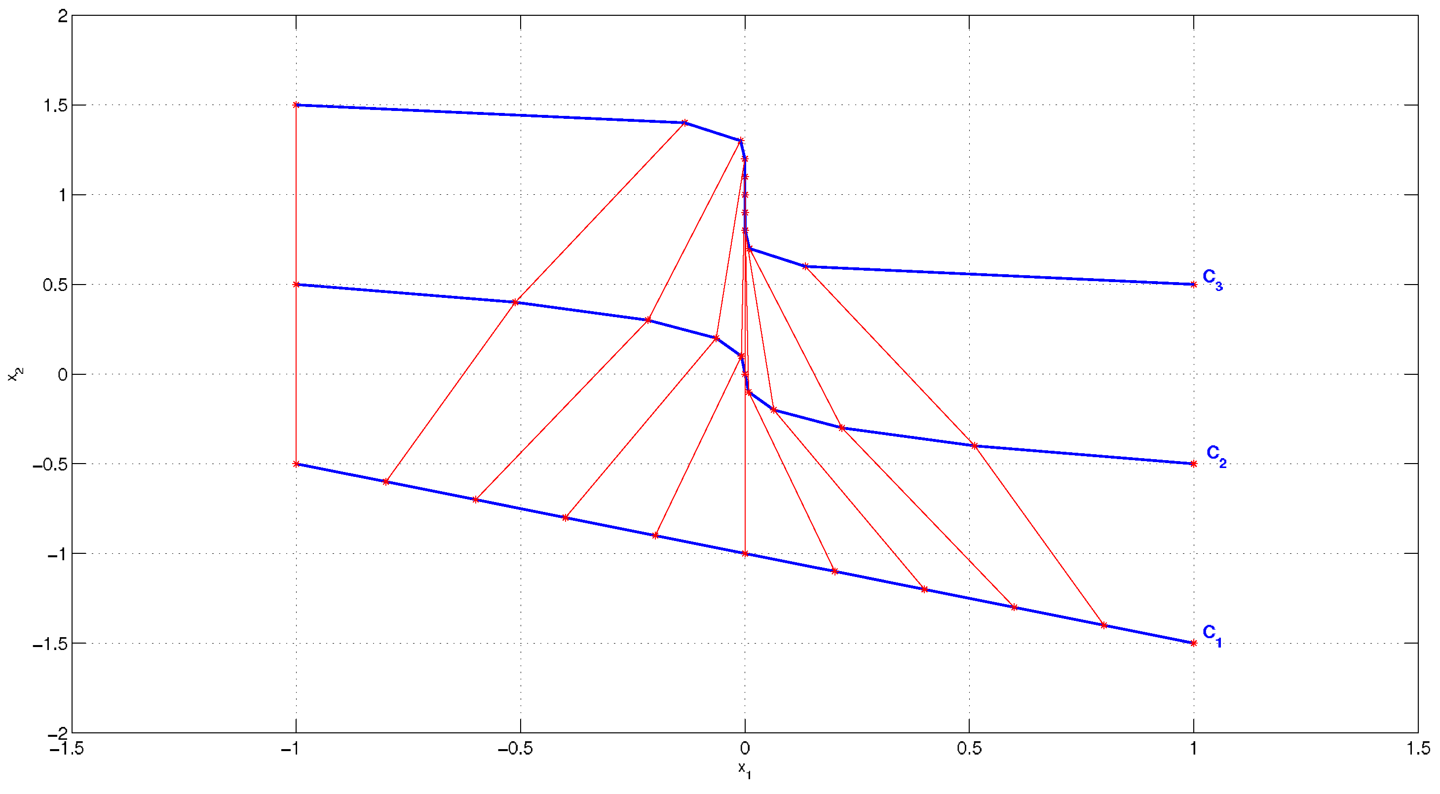
Let us consider a set of sample initial conditions for a dynamical system that are aligned along a straight line in the phase plane (or equivalently in the state space). The straight line connecting all the points has zero entropy, according to definition (6) in the previous section. As initial conditions evolve in the state space accordingly to the system dynamics, also the curve connecting them evolves, as shown in the example of figure 1. In particular, if points evolve according to linear dynamics, the entropy of the curve connecting them remains zero because collinearity is preserved under affine transformations. On the other hand, higher values of the entropy are a symptom of nonlinearity.

Figure 1. Evolution of a line in the phase space at three different time steps.

Figure 1. Evolution of a line in the phase space at three different time steps.

It should be remarked that the proposed approach does not compute the future trajectory of the initial line, but only the future trajectories of the initial points, and the line is derived consequently by connecting the points. According to this new approach, the upper bound of the indicator (6) depends now on the number of points that are used, so we normalise (6)

$$H_{norm}=\frac{H\left(\Gamma \right)-1}{log\left(N-1\right)},$$

(7)

where $N-1$ is the number of segments approximating the line, and the proof that the entropy computed according to (8) is bounded between zero and one is provided in Property 2, section 4. Also notice that at least two segments should be used, so that $N>2$ and indicator (8) has sense. By comparing equations (6) and (7) it is possible to obtain equation (8) to compute directly $H_{norm}$

$$H_{norm}=\frac{log\left({\displaystyle \frac{L}{d}}\right)}{log\left(N-1\right)}.$$

(8)

Notation $H_{norm}$ reminds that the entropy of a curve has been normalised, but from now on only the normalised value will be used and therefore the subscript $norm$ will be dropped for the sake of simplicity.

Assuming that a dynamical system evolves according to a discrete-time model

$$x\left(k+1\right)=f\left(x\left(k\right),k\right)x\in {\mathbb{R}}^m,$$

(9)

where m represents the dimension of the state vector, then the indicator (8) can be computed according to the following procedure

Algorithm 1:

• Initialisation: $k=0$

  (a)

  Choose N points $x_1\left(0\right),...,x_N\left(0\right)$ ordered along a straight line

  (b)

  $H\left(0\right)$ is 0

• Evolution: step k

  (a)

  Compute the next state for each point $x_1\left(k+1\right),...,x_N\left(k+1\right)$ according to (9)

  (b)

  Consider the line that connects sequentially all the points and take its length $L\left(k\right)$

  (c)

  Compute the smallest hypersphere that contains all the points, and take its diameter $d\left(k\right)$

  (d)

  Compute $H\left(k\right)$ according to (8)

  (e)

  Go to next step ( $k=k+1$ ).

Deterministic inputs can be included in equation (9) without significant changes, and have not been considered here for the sake of simplicity. Computation of the minimum covering sphere in point 2.c) is solved here using the approach of [14], and a brief discussion with the description of the algorithm is reported in the appendix for the sake of completeness.

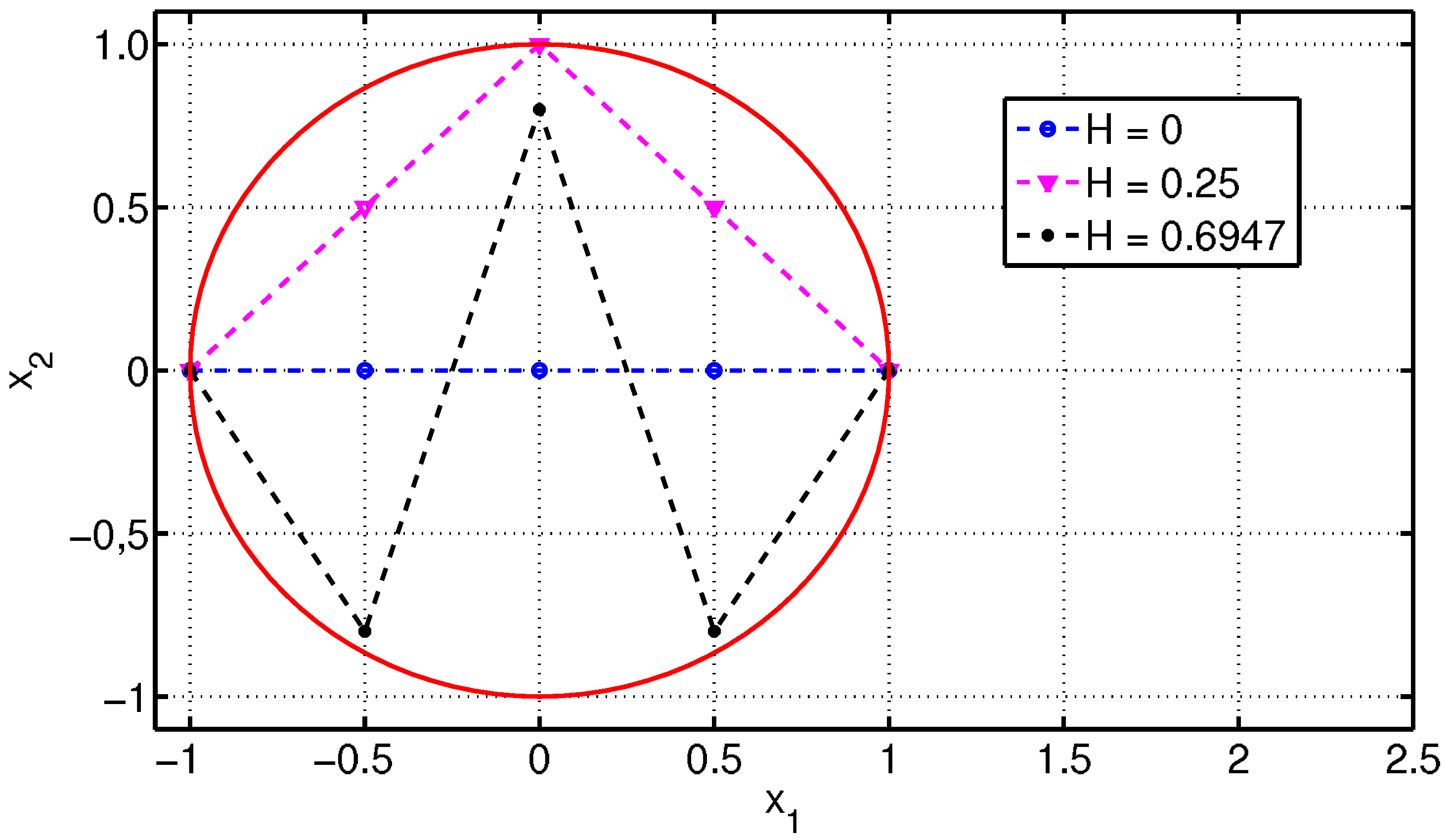
The rationale of indicator (8) is that it describes the regularity of a line: if all points are aligned sequentially along a straight line, then the segment has entropy 0. On the other hand, more tortuous lines have higher entropies, as illustrated in the example in figure 2.

Figure 2. Three plane lines covered by the same circle: more irregular lines have higher entropies.

Figure 2. Three plane lines covered by the same circle: more irregular lines have higher entropies.

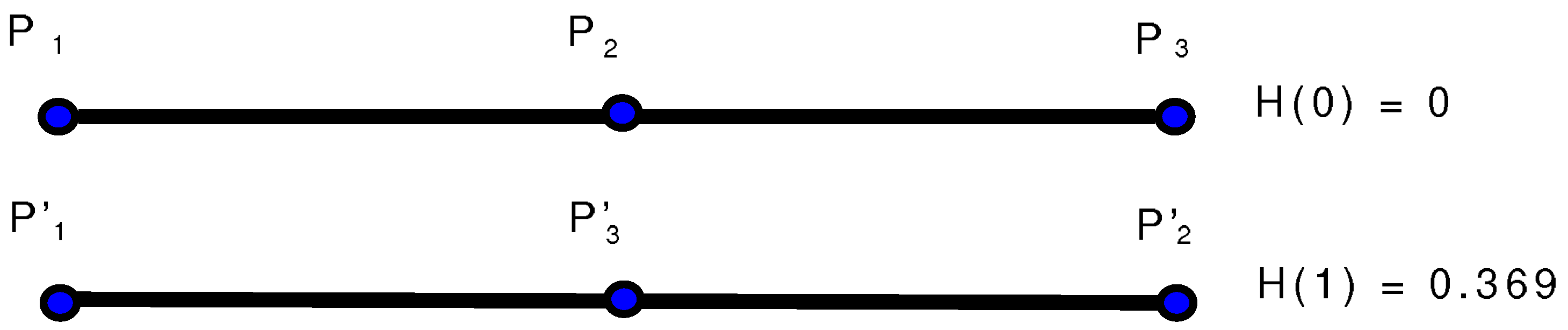
A second property is that the generalised entropy takes into account the ordering of the points in the sequence. This is described in Figure 3. At the beginning points $P_1$, $P_2$ and $P_3$ are chosen ordered along a straight line according to the first step of the previous algorithm. In this case $L=d=\overline{P_1{P}_3}$ and thus $H\left(0\right)=0$. If at the next step the system dynamics exchange $P_2$ and $P_3$, then $L=\overline{P_1^{{}^{\prime }}{P}_2^{{}^{\prime }}}+\overline{P_2^{{}^{\prime }}{P}_3^{{}^{\prime }}}$ while $d=\overline{P_1^{{}^{\prime }}{P}_2^{{}^{\prime }}}$. Therefore $H\left(1\right)>0$. By taking into account the ordering of the points, the generalised entropy is able to capture if the system dynamics are folding the initial segment over itself, which is clearly a symptom of nonlinearity.

Figure 3. A straight line turns into another straight line, but if the ordering of the points changes then the entropy changes as well.

Figure 3. A straight line turns into another straight line, but if the ordering of the points changes then the entropy changes as well.

The proposed indicator has many other interesting properties that make it suited for the analysis of dynamical systems, and they are described in the next section.

4. Properties of the generalised entropy

This section lists the main properties of the generalised entropy.

Property 1: Let Γ be a curve in ${\mathbb{R}}^n$, then the entropy of Γ is 0 if and only if Γ is a straight line.

Proof: The sufficient condition, i.e. a straight line has zero entropy according to (8) is easily verified. The necessary condition to be proved is that if $H=0$, and thus the diameter of the smallest hypersphere covering the curve Γ is equal to the length of Γ, then the only possibility is that the curve Γ is straight. To prove the necessary condition it should be noted that $\Gamma \subset A$, being A the hypersphere centered in the mid-point of Γ and diameter L equal to the lenght of Γ. Therefore, being the Minimum Covering Sphere (MCS) minimal, its diameter is always smaller or equal than L and, as a consequence of the fact that the MCS is unique, if $d=L$ then A must be the MCS. The curve Γ has at least two distinct points on the sphere surface, otherwise a smaller hypersphere can always be found. So, $d=L$ implies that Γ must have a point in the centre of the MCS and at least two on the surface. Now, since the overall length of Γ is d, then Γ must be formed by the two segments connecting the centre with the two points on the surface, otherwise it would be longer than just d by triangle inequality. In this case, the only possibility is that Γ is the diameter itself, otherwise the centre would not be a convex combination of the two points on the hypersphere surface, which is a necessary condition for the MCS [15]. Therefore the curve Γ corresponds to the diameter and it is a straight line.

Remark: This was the main property of the entropy of a plane curve and it still holds also for our generalised indicator.

Property 2: Let Γ be a curve in ${\mathbb{R}}^n$, then the entropy of Γ is always between 0 and 1.

Proof: As a consequence of the proof of property 1, the entropy of a curve Γ is bounded from below by 0. Besides, the maximum distance between two points within a hypersphere can not exceed the diameter. Thus, $L\le \left(N-1\right)·d$ and so $H\le 1$.

Remark: This property is guaranteed by the choice of the normalisation factor $log\left(N-1\right)$ in equation (8). The introduction of a normalising constant might not seem a proper choice because it affects the computation of the entropy of a curve. For instance, two identical curves described by a different number of points have now different entropies. However, from the point of view of dynamical systems analysis, it is convenient to have a fixed full scale range, although some care is required in providing the value of the entropy always accompanied with the information about the number of used points. Extensive simulations have been performed to investigate the sensitivity of equation (8) to the choice of the number of initial points and they showed that the asymptotic value of the entropy increases of one unit if the number of points doubles (i.e. it is proportional to the logarithm of the number of points). This result is in accordance with general intuition, for instance it directly follows from equation (8) if one assumes that the asymptotic distance between points does not depend on the number of considered points, and it is obviously true for the upper bound of the entropy as a consequence of property 2. Another important consequence of property 2 is that Algorithm 1 can be used consistently also to analyse unstable dynamical systems where the length of the curve tends to infinity. Finally, the normalisation step paves the way to a probabilistic approach.

Property 3: Let $\Gamma \left(k\right)$ be the curve in ${\mathbb{R}}^n$ at time step k generated by a dynamical system according to Algorithm 1. Then, if $\Gamma \left(0\right)=0$ then $\Gamma \left(k\right)=0$, $\forall k\in \mathbb{N}$ if the dynamical system is linear.

Proof: A linear system is described by the transition state function

$$x\left(k+1\right)=Ax\left(k\right)+b,$$

(10)

where A is a matrix and b is a vector of opportune dimensions, and (10) corresponds to an affine transformation of the vector $x\left(k\right)$. Collinearity and ordering of points are preserved under affine transformations, therefore a straight line remains a straight line and its entropy is constantly zero.

Remark: This property still holds for the approximation of the curve with arbitrary points, and it is the main reason why the entropy of curves is a valid tool for the analysis of dynamical systems. It should also be noted that the property is true even if the linear dynamical system (10) is time variant and includes deterministic inputs u (i.e. it is described by the more general equation $x\left(k+1\right)=A\left(k\right)x\left(k\right)+B\left(k\right)u\left(k\right)$). This more general case includes typical dynamical systems like for instance switching linear systems (provided that the switching condition is a function of time and not a function of the current state).

Property 4: Let Γ be a curve in ${\mathbb{R}}^n$, then the entropy of Γ is insensitive to scale changes, rotations and translations.

Proof: Entropy of a curve is defined as a ratio of lengths and therefore is not affected by scale changes. Furthermore, rotations and translations do not change lengths.

Property 5: Let $\Gamma \left(k\right)$ be the curve in ${\mathbb{R}}^n$ at time step k generated by a dynamical system according to Algorithm 1. If the dynamical system is one-dimensional, the state transition function is monotone and $\Gamma \left(0\right)=0$, then $\Gamma \left(k\right)=0$, $\forall k\in \mathbb{N}$

Proof: The proposed entropy indicator is based on the alignment or misalignment of a sequence of points. The case when the state space dimension is 1 is a degenerate situation in the sense that all the points remain necessarily aligned along the only (available) dimension. Therefore the proposed indicator only perceives the change of ordering of the points along the line, which is the only possibility for the entropy to be larger than 0, as it was shown in figure 3. The sequence of points does never change ordering if and only if $x_1\left(k\right)<x_2\left(k\right)$ implies $x_1\left(k+1\right)<x_2\left(k+1\right)$ (monotonically increasing) or implies $x_1\left(k+1\right)>x_2\left(k+1\right)$ (monotonically decreasing) for each choice of the points $x_1\left(k\right)$ and $x_2\left(k\right)$. Therefore, when the dynamical system has only one dimension the proposed entropy approach measures some way the monotonicity of the state transition function.

Remark: Even if the state function is not monotonic, the indicator might still be 0 if the initial segment is chosen in a region of the state space where the state function is monotonic. For instance, if an initial segment of ordered positive numbers is chosen and the state function is $x\left(k+1\right)=x{\left(k\right)}^2$, the non-monotonic behaviour of this system is missed.

Note 1: Following from the previous properties, one may think that nonlinear systems defined over dimensions greater than one always provide values of the entropy which are greater than zero. However, as already mentioned in property 3 the value of the entropy is constantly equal to zero for whatever choice of the initial line if the state transition function is such that transforms all straight lines into straight lines without affecting the ordering. The most famous class of transformations that preserve collinearity and ordering is indeed that of affine functions, which corresponds to the notion of linear dynamical systems. However degenerate dynamical systems that do not correspond to affine transformation can still be built ad hoc such that collinearity and ordering are preserved, as can be obviously seen in the next two-dimensional example:

$$\left\{\begin{array}{c}{x}_1\left(k+1\right)=x_1^3\left(k\right)\hfill \\ x_2\left(k+1\right)=x_1^3\left(k\right)\hfill \end{array}\right..$$

(11)

It could be argued however that dynamical systems like the previous one are intrinsically one-dimensional just the same.

Note 2: In this paper, we present an indicator that aims at evaluating the nonlinearity of dynamical systems. The indicator computes the entropy of a curve associated to a dynamical system (where the association comes into play because the curve evolves according to the system dynamics as described in Algorithm 1). Sometimes, for brevity, it is tempting to associate the entropy directly to the dynamical system. This shorter notation can however be misinterpreted with dramatic consequences because it conceals the fact that entropy is computed only of a curve. On the contrary, in our paper we never compute the entropy of the dynamical system, which is something completely different, and the entropy of curves does not inherit automatically the properties of the entropy as in the classic Boltzmann notion. As an example, one could expect that the entropy we compute here can never decrease, while this is not true because the entropy of curves evaluates the irregularity of a curve that, at least in principle, can decrease in time according to particular dynamic equations. Here, the term entropy is maintained for uniformity with the original notation [5,6].

The value of the proposed indicator can be computed either theoretically exploiting the previous properties and theorems, or by Algorithm 1. The theoretical approach can be used if the dynamical system is linear to infer that the entropy will be constantly zero, or if the dynamical system has symmetric properties that lead to a geometrical solution. For instance, if the nonlinear system is $x\left(k+1\right)=x{\left(k\right)}^2$, then an initial line symmetric with respect to the origin will fold up on itself so that (8) will be $log\left(2\right)/log\left(N-1\right)$.

If the dynamical system does not have particular symmetries or properties, it will be generally very hard to predict the behaviour of the indicator and it is necessary to use the algorithmic procedure. On the other hand, a drawback of Algorithm 1 is that it might be numerically unstable if the points converge all to an equilibrium or diverge. In the first case, all distances among the points go to zero, while in the second case they go to infinity. For this reason, the algorithmic procedure gives the best results in the case that the norms of the state points remain bounded and do not converge to one only value. A possible application is therefore the analysis of chaotic systems, when the states evolve within attractors. Besides, literature of chaotic systems is rich of indicators that are used to quantify the amount of chaoticity, starting from the well-known Lyapunov exponents. It is therefore of interest to investigate how the proposed indicator is related with the other approaches.

5. Analysis of Chaotic Behaviours

The generalised entropy indicator introduced in this work can be computed in an algorithmic way which is particularly convenient for the evaluation of chaotic behaviours. Chaotic behaviours have been widely studied in the recent years, and methods like the Lyapunov Exponents (LEs), the auto-correlation function and the power spectrum have become classic tools of chaos theory [4]. Other less conventional indicators have been introduced in the last few years, as for instance [16,17,18] and the very recent [19]. However, no approach has prevailed over the others yet, since depending on the particular dynamical system, or on the particular aspect of interest, one method can be more convenient and more informative than the others.

The different indexes try to quantify the amount of chaos by observing the evolution of different quantities. In this framework the entropy approach proposed here is closely related to LEs and to the $d_{\infty }$ parameter introduced in [20,21], since they are both concerned on the evaluation of some distances, as will be clarified in the following.

The maximum LE [22] gives a quantitative characterization of the exponential divergence of initially nearby trajectories. Similarly to the entropy approach, it is not generally possible to compute LEs in an analytic way, but one has to resort to numerical methods. LEs are computed evaluating the evolution of some points in the phase space, and two recent references for computation in continuous time systems and discrete time can be found in [23] and [24] respectively. A recent survey of the theory of Lyapunov exponents is also available from [25]. A drawback of LEs is that two dynamical systems having the same LEs can behave in a very different way [26]. In particular, if a chaotic system in ${\mathbb{R}}^n$ is characterised by LEs ${\lambda }_1,{\lambda }_2,...,{\lambda }_n$, then a linear continuous dynamical system with state transition matrix $A=diag\left[{\lambda }_1,{\lambda }_2,...,{\lambda }_n\right]$ has the same LEs. Although it is still true that two trajectories arbitrarily close diverge in the long term if the dynamical system is linear and unstable, yet the behaviour is far from chaotic. This is a major difference with respect to the proposed generalised entropy indicator. A second drawback of LEs is that it is not clear how to compute them for dynamical systems defined over a discrete state space. In this case, it is not straightforward how to define the distance between two states and whether two trajectories converge or not. On the contrary, the proposed generalised indicator provides a nice extension for the investigation of unusual dynamical systems defined on a discrete state space, as for instance the Kaprekar routine [27] addressed in the next section.

The parameter $d_{\infty }$ was first introduced in [20] and measures the asymptotic distance between trajectories. An iterative procedure to compute the value of $d_{\infty }$ starts from the choice of several pairs of initial conditions. The mean distance $d_j$ between two trajectories after j iterations can be computed as

$$d_j=\frac{1}{N}\sum _{i=1}^N∥x_j^{\left(i\right)}-x_j^{{}^{\prime }\left(i\right)}∥,$$

(12)

where, using the same notation of [21], $x_j^{\left(i\right)}$ and $x_j^{{}^{\prime }\left(i\right)}$ are the pair i (out of the total of N) of points at iteration j. Finally $d_{\infty }$ is computed by averaging $d_j$ after n iterations, when n tends to ∞. The previous approach can be used for the analysis of chaotic dynamical systems, where the distance reaches a characteristic asymptotic value [21] that has lost memory of the initial conditions [28]. In [21] it is not outlined how the initial points of a pair should be chosen, apart from being very close one to the other. If it were possible to choose all of them along a line, then the asymptotic entropy according to the equation (8), here called for analogy $H_{\infty }$, would be

$$H_{\infty }=\frac{log\left({\displaystyle \frac{\left(N-1\right)d_{\infty }}{diam}}\right)}{log\left(N-1\right)},$$

(13)

where, to avoid confusion with the mean distance $d_j$ (12), we call $diam$ the diameter of the smallest hypersphere that encloses all the points (which in equation (8) had been called d). It should be noted that also $diam$ reaches an asymptotic value, since after the first steps, the points get spread enough to cover the whole attractor. Therefore a proportional relationship between the logarithm of $d_{\infty }$ and the entropy indicator proposed here gets established. In [21], a relationship between $d_{\infty }$ and the maximum LE is computed according to the equation

$$d_{n+1}=\Lambda d_n-\Psi d_n^2,$$

(14)

where $log\left(\Lambda \right)$ is the maximum Lyapunov exponent, and Ψ represents the folding action. Therefore, asymptotically, apart from the simple solution $d_{\infty }=0$, the fixed point is $d_{\infty }=\frac{{\displaystyle \Lambda -1}}{{\displaystyle \Psi }}$. The previous relationship emphasises the fact that the maximum LE measures the stretching effect, while $d_{\infty }$ takes into account also the folding aspects through the term Ψ. However, during the first steps the stretching effect is dominant over the folding one, and thus the rate of growth of the initially small distance $d_0$ is directly related to the maximum LE. In [29] an empirical way of estimating the maximum LE from the evolution of $d_j$ is suggested, although results are not very accurate. However this is important to remind, because it points out that not only the asymptotic value of the entropy of curves is an interesting parameter, but also the entropy rate provides significative information of the underlying dynamics.

Finally, it is remarked that the previous relationships between LEs, $d_{\infty }$ and the entropy indicator only hold when the dynamical system is chaotic.

6. Results and Discussion

Extensive simulations have been performed to study the behaviour of the proposed index in many benchmark problems. In the following, some of the most significant results that have been obtained are presented and compared.

Figure 4. Comparison of the entropy of curves computed for a two-state dynamical system as a function of the probability of changing the state.

Figure 4. Comparison of the entropy of curves computed for a two-state dynamical system as a function of the probability of changing the state.

An interesting example is the case when the state can either be 0 or 1. At each time step the state remains the same or changes as according to the outcome of a Bernoulli experiment. The generalised entropy computed in this situation is larger when the two probabilities of remaining in the same state and switching to the second one are close one to each other, as shown in figure 4. This is in analogy with the entropy as in information theory, [13] and [30], and emphasises that the proposed indicator takes into account the predictability of a dynamical system. Indeed, a probability of $50\%$ of switching the state represents the most unpredictable situation and is characterised by the highest entropy.

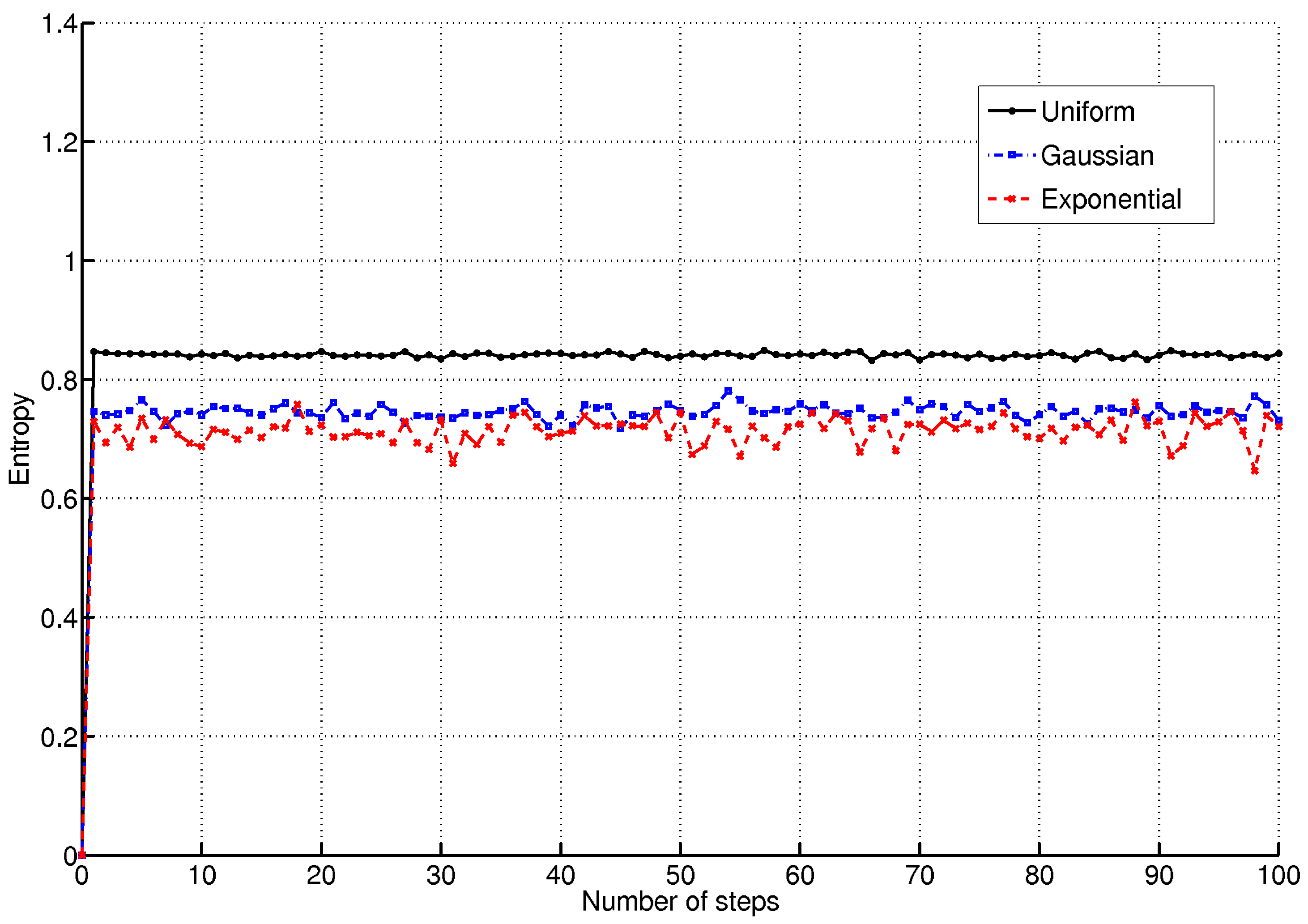
Figure 5. Comparison of the entropy of curves associated to some probability distributions. Highest entropies are reached respectively by the exponential, the Gaussian and then the uniform distribution.

Figure 5. Comparison of the entropy of curves associated to some probability distributions. Highest entropies are reached respectively by the exponential, the Gaussian and then the uniform distribution.

A similar example is shown in figure 5, where entropies of curves associated to several probability distributions are compared. In this case the dynamical system is described by the equation

$$x\left(k+1\right)\sim \mathcal{P}\left(x\right),$$

(15)

where ’$\sim \mathcal{P}$’ means that the state is sampled according to the probability distribution $\mathcal{P}$. In the comparison three different simulations have been performed, where the state is sampled according to a uniform, Gaussian and exponential probability distribution respectively. It should be noted that it is possible to associate an entropy of curves to a distribution without specifying the typical values characterising a distribution. This implies for instance that it is not necessary to specify the bounds of the uniform distribution, because the entropy is insensitive to translations or changes of scales, according to property 4 in the previous section. Similarly, in the Gaussian case, the entropy does not depend on the mean or on the variance and in the exponential case it does not depend on the mean or on the value of the parameter μ. Dynamical systems (15) are characterized by the loss of memory of the previous state, but in the Gaussian and in the exponential cases lower entropies are achieved since samples have higher probabilities the closer they are to the mean value. On the other hand, the uniform case represents the least predictable dynamical system.

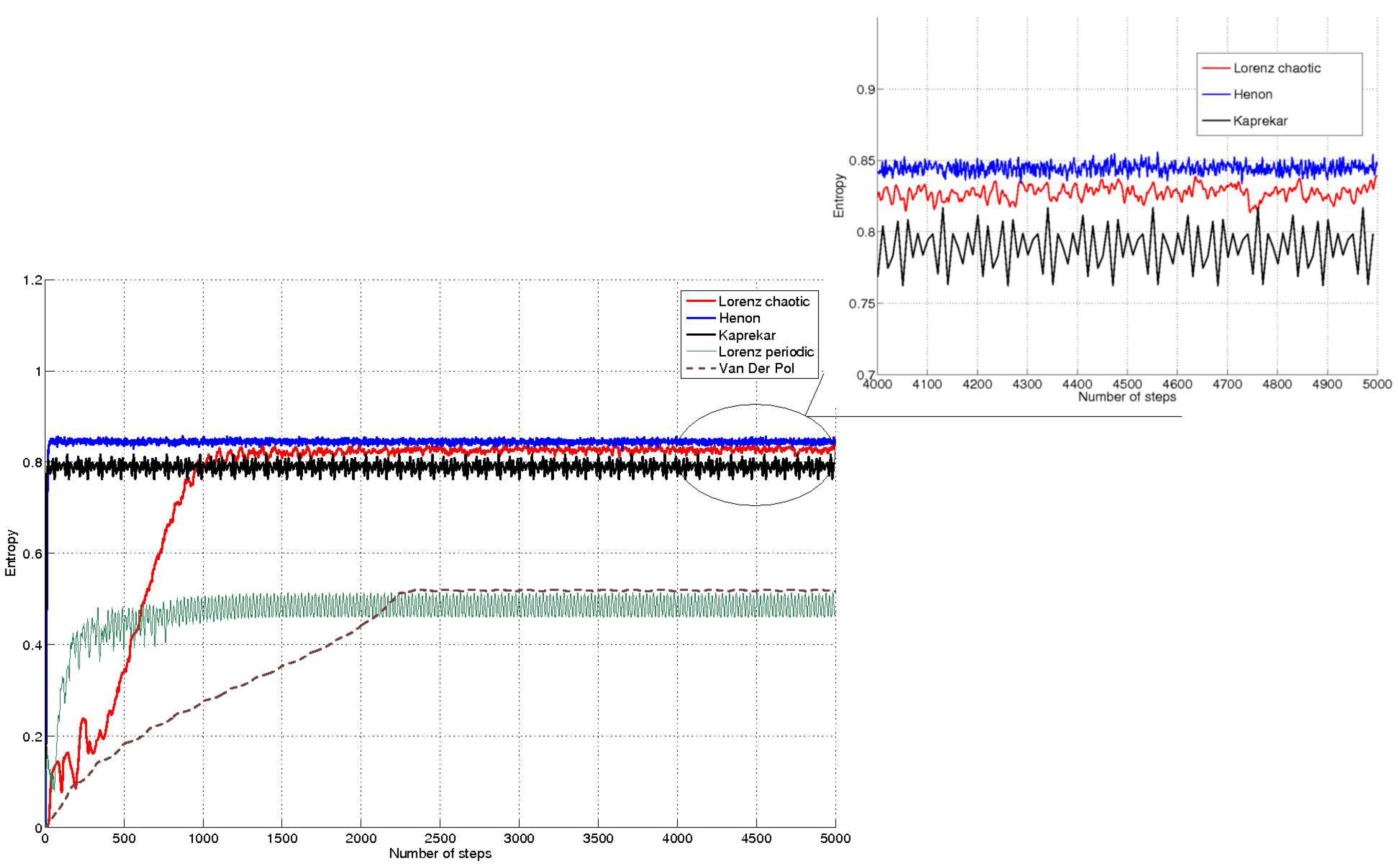
Figure 6 compares several dynamical systems, such as Lorenz attractor, Hénon map, Van Der Pol oscillator and Kaprekar routine. Lorenz equations are described by

$$\left\{\begin{array}{c}\dot{x_1}=-\sigma \left(x_1-x_2\right)\hfill \\ \dot{x_2}=R{x}_1-x_2-x_1{x}_3\hfill \\ \dot{x_3}=x_1{x}_2-b{x}_3\hfill \end{array}\right.,$$

(16)

and have been discretised with a sampling time of $0.01$ s. In a first example the chaotic behaviour of the equations was obtained by choosing the classic values $\sigma =10$, $R=28$ and $b=8/3$. In a second example a periodic solution of the Lorenz equations is obtained by choosing $R=260$. Hénon map is described by

$$\left\{\begin{array}{c}{x}_1\left(k+1\right)=x_2\left(k\right)+1-a{x}_1^2\left(k\right)\hfill \\ x_2\left(k+1\right)=b{x}_1\left(k\right)\hfill \end{array}\right.,$$

(17)

where the typical values $a=1.4$ and $b=0.3$ have been used. Van Der Pol oscillator is described by:

$$\left\{\begin{array}{c}\dot{x_1}=x_2\hfill \\ \dot{x_2}=\left(1-x_1^2\right)x_2-x_1\hfill \end{array}\right.,$$

(18)

where a discretisation step of $0.01s$ has been used again.

Figure 6. Comparison of the entropy of curves for some dynamical systems. Higher entropies are achieved respectively by the chaotic Hénon map, Lorenz equations in the chaotic case and Kaprekar routine. Lower entropy values are reached by the Van Der Pol oscillator and Lorenz equations in the periodic case.

Figure 6. Comparison of the entropy of curves for some dynamical systems. Higher entropies are achieved respectively by the chaotic Hénon map, Lorenz equations in the chaotic case and Kaprekar routine. Lower entropy values are reached by the Van Der Pol oscillator and Lorenz equations in the periodic case.

The same notation of [4] was used to describe the previous dynamical systems. Finally, Kaprekar routine [27] consists of an algorithm that can be applied to integer numbers and works performing alternately the following steps:

Step 1 

Rearrange the digits of a number $a\left(k\right)$ in ascending and descending order so to obtain two new numbers $\underline{a}\left(k\right)$ and $\overline{a}\left(k\right)$ respectively.

Step 2 

Compute $a\left(k+1\right)=\overline{a}\left(k\right)-\underline{a}\left(k\right)$. Increase time index k and go back to step 1

In the example, Kaprekar routine has been applied to ten digit numbers. All the previous examples are compared in figure 6, where $N=1000$ points have been used in all the examples.

Remark: It might be argued that a comparison among so different dynamical systems is somewhat artificial. For instance, Lorenz equations have three states, the Hénon map and the Van Der Pol oscillator have two states and Kaprekar routine has one only dimension. Two of them are continuous time dynamical systems (although discretisation is performed) and two of them are discrete time. Moreover the Kaprekar routine is described by non-continuous equations and its domain is a discrete set. What is meant to show here is the flexibility of the proposed algorithm, which can be used efficiently to describe the nonlinear behaviour of classic continuous dynamical systems as well as less conventional dynamics like the Kaprekar routine. Not the same holds for other approaches like Lyapunov exponents.

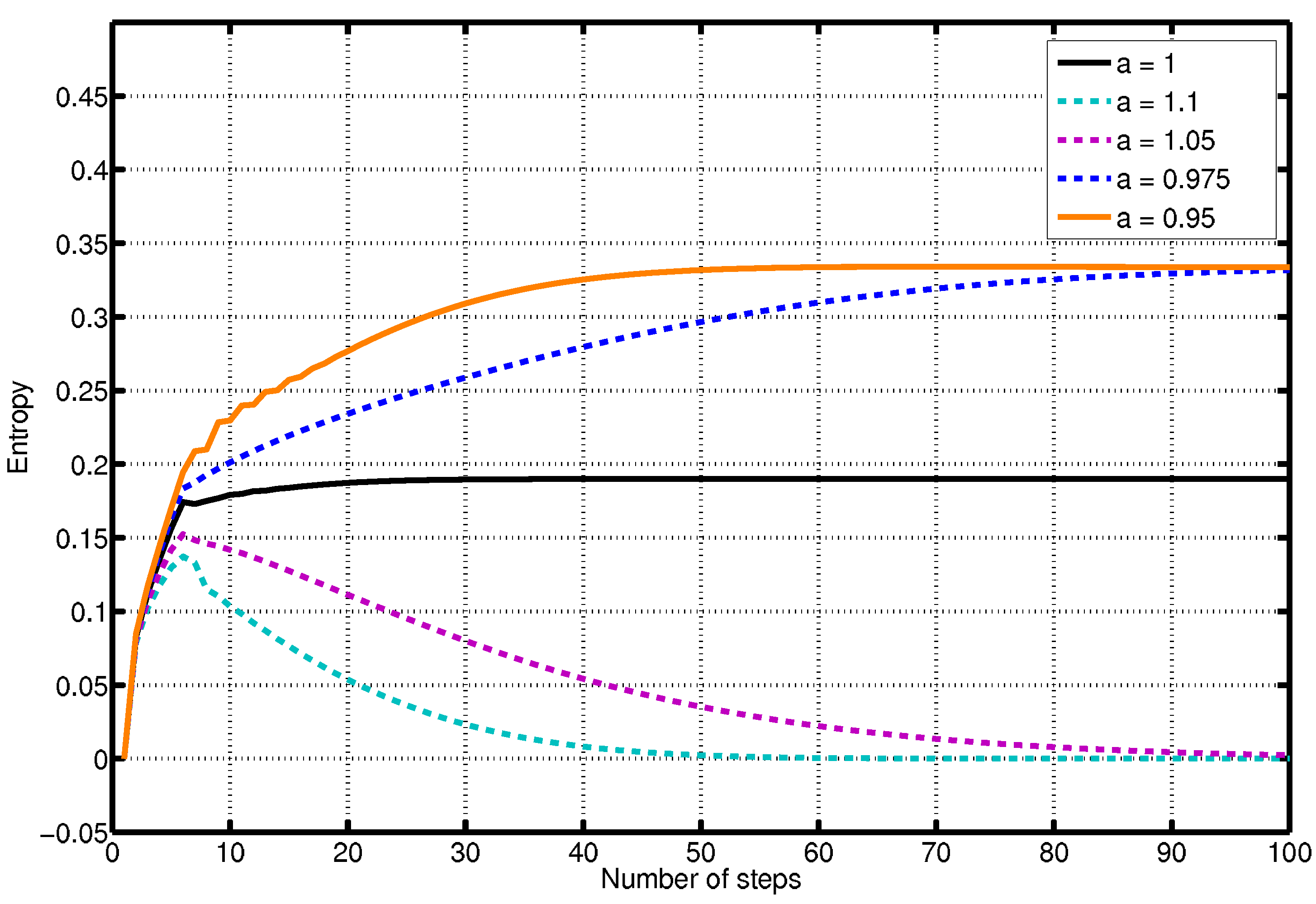
The next example is dedicated to the comparison of the entropy indicator for a dynamical system where a parameter a is used to tune the amount of nonlinearity. The investigated dynamical system evolves according to the equations:

$$\left\{\begin{array}{c}{x}_1\left(k+1\right)=a·x_1\left(k\right)\hfill \\ x_2\left(k+1\right)=3.2·x_2\left(k\right)·\left(1-x_2\left(k\right)\right)\hfill \end{array}\right..$$

(19)

The first component of the system (19) evolves with linear dynamics, so its expected entropy is 0. The second component evolves according to a logistic equation, which is a function that can be used to represent demographic models, where the multiplicative parameter is a positive number representing a combined rate for reproduction and starvation [3]. In the example here the value of the parameter is $3.2$, and the equation has two equilibrium points. In the example, when $\left|a\right|<1$, the linear component goes to zero and the dynamical system reduces to the nonlinear part. On the contrary, when $\left|a\right|>1$, the linear component overrides the nonlinear one. Finally when $\left|a\right|=1$ the two components have comparable values. The entropy of the system reflects this situation, and it either assumes the value of the dominant component or an intermediate value in the last case.

The simulation results are shown in figure 7, where the higher entropies are reached when a has values $0.95$ and $0.975$ (nonlinear dominance). The curves converging to 0 entropy are due to values of a equal to $1.1$ and $1.05$ (linear dominance). The curve in the centre is obtained when $a=1$. In addition, it can be noted that the value of a affects the time that is necessary before the linear component becomes dominant or can be neglected, therefore affecting the transient behaviour of the entropy. Also notice that in the case that the linear component prevails over the nonlinear one the entropy recognises the nonlinearity (the entropy indicator is not constantly zero), and then it decreases to zero. The fact that the entropy decreases implies that the curve in the phase space after the first few steps becomes more regular.

Figure 7. Comparison of the entropy of curves indicator applied to a dynamical system in function of a parameter that weighs the contributions of the linear and nonlinear components

Figure 7. Comparison of the entropy of curves indicator applied to a dynamical system in function of a parameter that weighs the contributions of the linear and nonlinear components

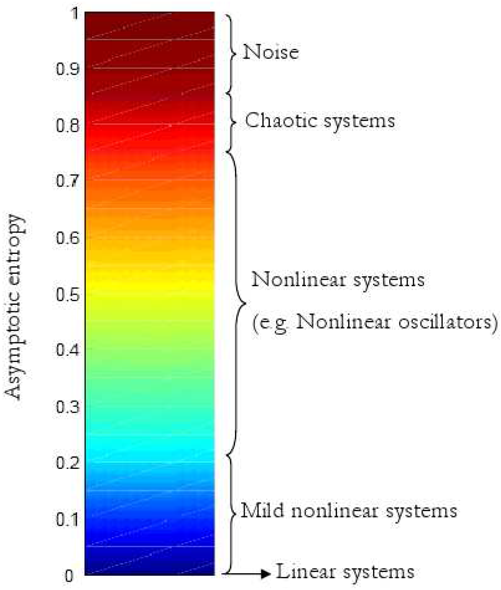
Figure 8. A thermometer is used to classify dynamical systems according to the asymptotic value of the associated entropy of curves.

Figure 8. A thermometer is used to classify dynamical systems according to the asymptotic value of the associated entropy of curves.

The results shown so far associated a particular value of the entropy of curves to a dynamical system without specifying the choice of the initial line. Extensive simulations have been performed to prove that dependence on the initial conditions, for instance the direction or the length of initial line is not relevant. This is the case of many nonlinear systems, as those previously investigated, provided that the initial condition is chosen within the state space region of interest, for instance the attractor set for chaotic systems. In such situations, the entropy indicator manages to describe some nonlinearity properties of the dynamical system in exam, and simulation results were used to build up a thermometer with several degrees of nonlinearity associated to nonlinear behaviours, as shown in figure 8.

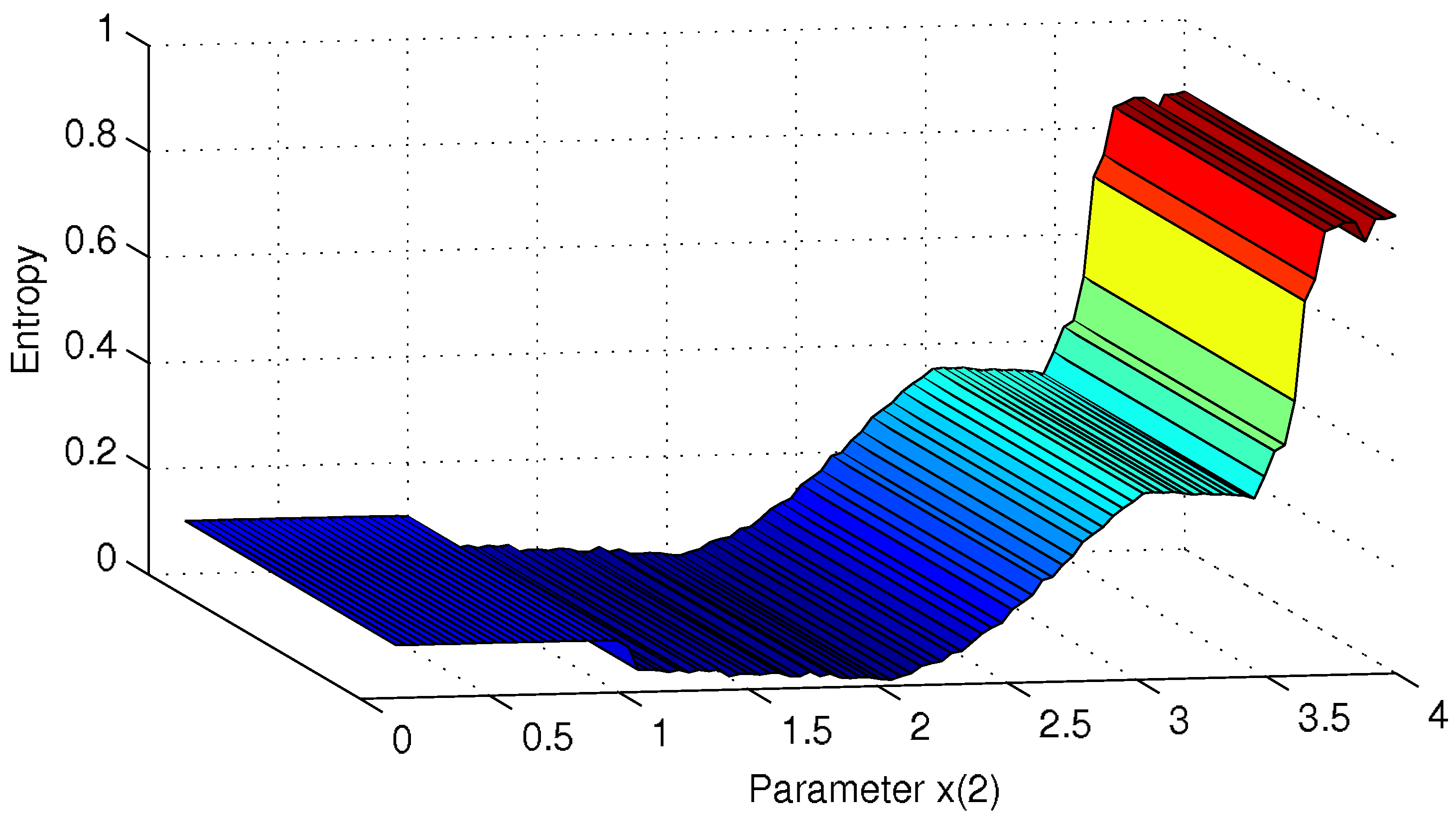
According to simulations, noise and chaotic systems often have similar asymptotic entropy, and therefore are assumed to have comparable degrees of nonlinearity. However uniform noise and Bernoulli experiments with equal probabilities have higher entropy than chaotic systems. Entropies higher than $0.9$ are not usually reached, although dynamical systems can be designed on purpose so that values of the entropy close to the limit of 1 can be achieved. Finally it is reminded that 0 entropy is achieved by all possible linear (arbitrarily time variant and unstable) dynamical systems. However, this thermometer is far from encompassing all possible nonlinear behaviours. For instance, in many situations the initial conditions (i.e. the first straight line) can affect the generalised entropy indicator and its final value, and therefore it does not make sense to associate the indicator to a dynamical system, since it depends on some initial choices. This can be unavoidable if the behaviour of the nonlinear system depends on the initial conditions as well. In this case Monte Carlo choices of the initial conditions might be necessary to distinguish among different behaviours of the same nonlinear system. As an example of this situation the logistic equation is considered in the case that the state is extended to include the fixed rate parameter:

$$\left\{\begin{array}{c}{x}_1\left(k+1\right)=x_2\left(k\right)·x_1\left(k\right)\left(1-x_1\left(k\right)\right)\hfill \\ x_2\left(k+1\right)=x_2\left(k\right)\hfill \end{array}\right..$$

(20)

It might sound misleading to describe a one dimensional system as the logistic map as a two dimensional one as in (20) (although please note that this is artificial because the second state does not evolve). This is done here to propose a well-known example where the behaviour of the dynamical system depends on the initial conditions in the phase space. This is not true in the conventional notation where the parameter is not considered as a state. It is known from literature [3] that the logistic function presents both stable and chaotic behaviours depending on the initial value of the parameter ($x_2$ according to the notation of (20)). Namely, system (20) has one equilibrium when $x_2\left(0\right)$ is smaller than 3, it oscillates for parameter values between 3 and $3.57$ (approximately), and shows a chaotic behaviour for values greater than $3.57$ and smaller than 4. There is a so-called “island of stability" for values around $3.8$ and finally it diverges for almost all initial conditions when the parameter is greater than 4. Therefore it is not very sensible to evaluate the dynamical system (20) with one only indicator, but it is reasonable to compute the entropy indicator as a function of the initial condition of the second component. The graph of the entropy indicator so obtained is summarised in figure 9 and reproduces realistically the known behaviour of the logistic function. Figure 9 shows the linear interpolation of the values of the asymptotic entropies computed for values of the parameter from $0.1$ to 4 with a $0.04$ interval step.

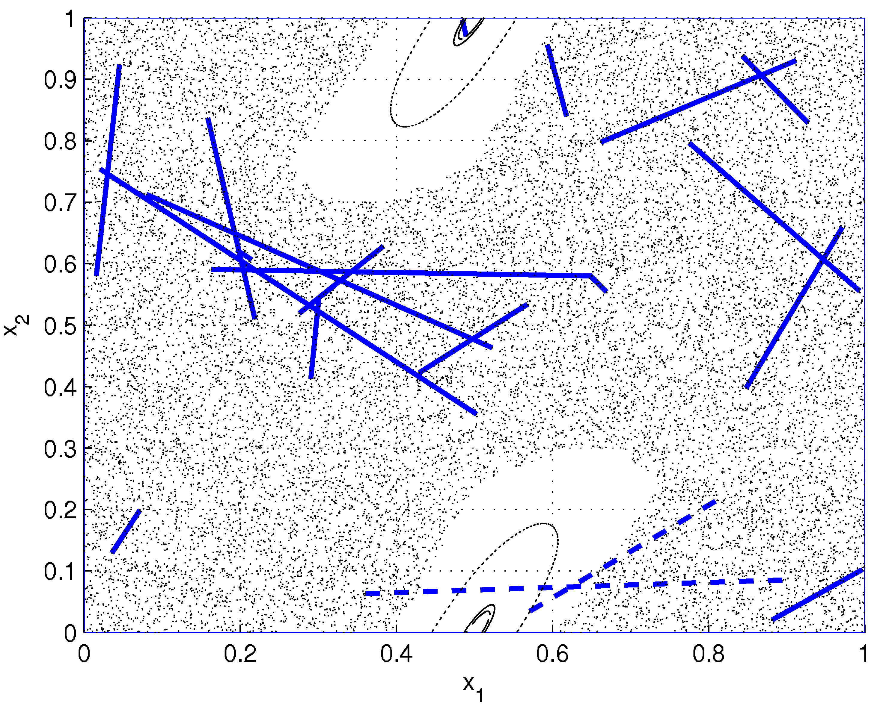
Following the same motivations of the previous example, a last problem is presented now where the behaviour of the dynamical system depends again on the special region of the phase space. This example is known as the standard map, and it is of particular interest in the nonlinear science and it corresponds to a conservative system where both order and chaos coexist. In fact, the phase space is composed at the same time of one large island of stability and a large connected chaotic domain [31]. Dynamical equations are

$$\left\{\begin{array}{cc}{x}_1\left(k+1\right)=x_1\left(k\right)+x_2\left(k+1\right)\hfill & (mod1)\hfill \\ & \\ x_2\left(k+1\right)=x_2\left(k\right)+\frac{{\displaystyle K}}{{\displaystyle 2\pi }}sin\left(2\pi x_1\left(k\right)\right)\hfill & (mod1)\hfill \end{array}\right.,$$

(21)

where here $K=3$ is used, so to discuss the example of [31] with the same value of the parameter. In this case, we choose 20 random initial segments inside the unit square, and 1000 random points within each segment. Figure 10 shows the initial segments, and the trajectories followed by the end-points of the segments. The trajectories followed by the end-points of the segments lying initially inside the island of stability can be followed easily by inspection, while points evolving in the chaotic region fill the region apparently homogeneously without following distinguishable orbits.

Figure 9. Comparison of the entropy indicator of the logistic equation as a function of the parameter.

Figure 9. Comparison of the entropy indicator of the logistic equation as a function of the parameter.

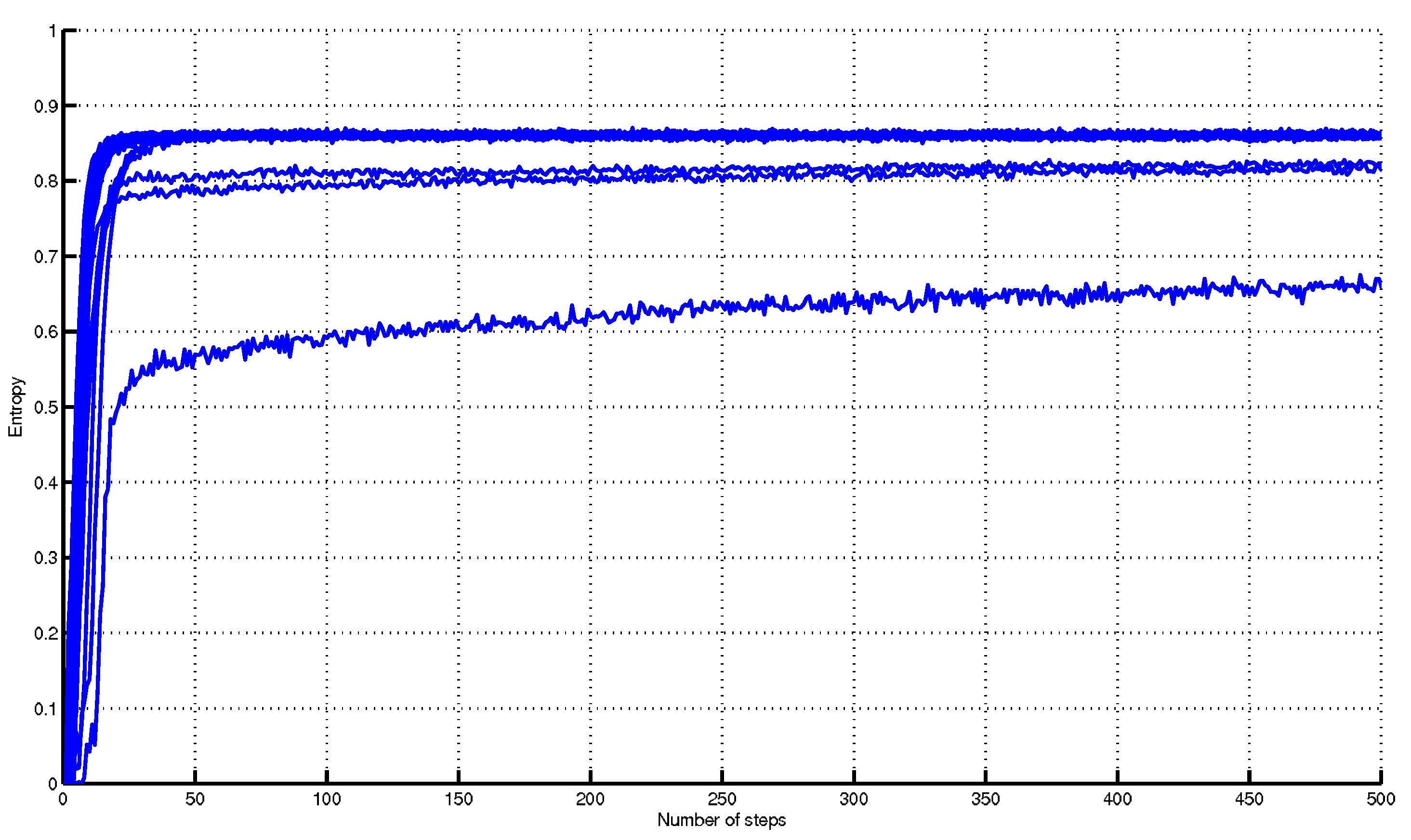
The 20 evolutions of the entropy are recorded and shown in figure 11, where one entropy graph is clearly different from the others. As one might imagine, it corresponds to the initial condition of the segment inside the island of stability (in figure 10 it corresponds to the small segment on top of the figure).

Moreover, there are other two entropy graphs slightly different from the others, and they correspond to the two dashed segments that partially cross the island of stability. While it is straightforward to classify the initial conditions from figure 11, the same does not occur if one just compares the values of the asymptotic entropies as a function of the initial conditions. In fact, it might be surprising to find that all entropy graphs saturate to the same final value, corresponding to that of the other 17 initial segments of figure 11 if a longer observation time range is chosen. Differently from all the previously studied examples, the information of the rate of growth of the generalised entropy (or alternatively the whole generalised entropy curves) should here be considered together with the asymptotic values to distinguish the initial conditions. Simulations show that the reason why entropy keeps increasing is that although trajectories associated to each initial point inside ordered regions look very regular, points progressively exchange their relative positions, also due to the $mod$ functions appearing in equations (21), and thereby affect the value of the generalised entropy. Also notice that generalised entropy saturates to an asymptotic value and therefore its rate of growth can not be constant, as it is expected because the H index is bounded from above as previously proved in Property 2. A final observation to say that the final value of convergence is very close to the one that is obtained in the case of uniform noise in example 5, so it suggests that in the end the motion of the points is as nonlinear as if driven by a random motion with uniform distribution, independently from the initial conditions.

Figure 10. Evolution of trajectories of points according to the standard map. Initial segments and the trajectories followed by one of their endpoints are also shown.

Figure 10. Evolution of trajectories of points according to the standard map. Initial segments and the trajectories followed by one of their endpoints are also shown.

Figure 11. Evolutions of the entropy for the 20 segments randomly chosen inside the unit square. The initial choice of the segments (whether inside or outside (or even crossing) the island of stability) clearly affects the entropy.

Figure 11. Evolutions of the entropy for the 20 segments randomly chosen inside the unit square. The initial choice of the segments (whether inside or outside (or even crossing) the island of stability) clearly affects the entropy.

7. Conclusions

This paper provides a generalised definition of the entropy of a curve and an algorithmic procedure to compute it. Moreover, the generalised indicator derived from the thermodynamics of curves is proposed to analyse the evolution of a curve in the phase space and infer some properties of the underlying dynamical system. The proposed indicator is proved to be bounded between 0 and 1 and it is constantly 0 if the dynamical system is linear. Several nonlinear systems, having completely different characteristics have been compared and classified according to the entropy index. In particular, examples show that the entropy indicator takes into account difficulties in predicting the evolution of dynamical systems and is able to quantify the amount of nonlinearity of linear/non linear systems. Finally, the generalised entropy is used to analyse chaotic systems, and some similarities with other known indicators were presented. In case of chaotic systems, the generalised entropy is also an alternative choice to Lyapunov Exponents, both because it reveals other aspects of the underlying dynamical system (i.e. it quantifies the stretching and the folding aspects at the same time) and because it extends the application field to the investigation of dynamical systems defined on a discrete state space. The proposed indicator has many useful properties and provides very promising results with a wide generality. Nevertheless, a systematic way to classify nonlinear systems in their whole generality is still an unsolved problem because a nonlinear system might present very different behaviours (stability, instability, limit cycles, attractors..) in different regions of the state space. In these situations it might be required to compute the entropy as a function of a parameter, as in the logistic example presented in the previous section, since it is not sensible to associate a unique nonlinearity value to a complex dynamical system where more behaviours coexist at the same time. Besides, the rate of growth of the entropy is another interesting parameter to evaluate dynamical systems, due to the theoretical reasons explained in section 5. In the last example for instance, it helps to discriminate different behaviours within the same dynamical system.

Although the proposed indicator derived from the theory of the entropy of plane curves is intended to discriminate linear from nonlinear systems and provide a degree of nonlinearity, there seems to be more interest to exploit its potentialities for the special case of the investigation of chaotic dynamical systems. For this reason, future lines of research will focus on the joint evaluation of the entropy and rate of entropy to analyse chaotic systems, as in the last proposed example, and compare the achieved results with the other (many) chaotic indicators from the literature.