Gravitational Entropy and Inflation

Abstract

The main topic of this paper is a description of the generation of entropy at the end of the inflationary era. As a generalization of the present standard model of the Universe dominated by pressureless dust and a Lorentz invariant vacuum energy (LIVE), we first present a flat Friedmann universe model, where the dust is replaced with an ideal gas. It is shown that the pressure of the gas is inversely proportional to the fifth power of the scale factor and that the entropy in a comoving volume does not change during the expansion. We then review different measures of gravitational entropy related to the Weyl curvature conjecture and calculate the time evolution of two proposed measures of gravitational entropy in a LIVE-dominated Bianchi type I universe, and a Lemaitre-Bondi-Tolman universe with LIVE. Finally, we elaborate upon a model of energy transition from vacuum energy to radiation energy, that of Bonanno and Reuter, and calculate the time evolution of the entropies of vacuum energy and radiation energy. We also calculate the evolution of the maximal entropy according to some recipes and demonstrate how a gap between the maximal entropy and the actual entropy opens up at the end of the inflationary era.

1. Introduction

The importance of gravity for the establishment of an arrow of time in the Universe was emphasized by P. C. W. Davies [1] in an article entitled Inflation and the time asymmetry in the Universe. He noted that gravity, when it is attractive, tends to contract matter and, if possible, make black holes. In this case, a smooth distribution of matter represents a small gravitational entropy.

However, if gravity is repulsive, so that it tends to smoothen the distribution of matter and energy, it seems natural to say that a state with an irregular mass distribution would be a low entropy state and a smooth state would be one of maximum entropy. Under attractive gravity, an inhomogeneous clumped field has high entropy, but with the switch to repulsive gravity, it is redefined as low entropy. Concentrations of mass, i.e., curvature, try to smooth themselves out, and the gravitational field tends towards uniformity.

This way of talking about gravitational entropy is in accordance with the second law of thermodynamics, securing that gravitational entropy increases during a period dominated by repulsive gravity. However, it is in conflict with the definition of gravitational entropy defined as an expression of the inhomogeneity of a gravitational field. A general agreement as to how one should define and describe mathematically the gravitational contribution to the cosmic entropy during a period dominated by repulsive gravity has not yet been obtained.

Before the Planck time, ${10}^{-43}$ s, the Universe was probably in a state of quantum gravitational fluctuations. Then, it entered an inflationary era lasting about ${10}^{-33}$ s, dominated by dark energy with a huge density, possibly in the form of Lorentz invariant vacuum energy (LIVE). The Universe then evolved exponentially fast towards a smooth and maximally symmetric de Sitter space, which represents the equilibrium end state with maximal entropy when the evolution is dominated by a non-vanishing cosmological constant. This was an essentially adiabatic expansion with small changes of entropy.

At the end of the inflationary era, the entropic situation changed abruptly. The vacuum energy was transformed to radiation and matter; gravity became attractive, and it became entropically favorable for the Universe to grow clumpy. As pointed out by Veneziano [2], in any inflationary scenario, most of the present entropy is the result of these dissipative processes. However, not only did the entropy of the matter increase, as calculated in Section 7, the value of the maximum possible entropy also increased—and much more than the actual entropy. Hence, a large gap opened between the actual entropy of the Universe and the maximum possible entropy of the Universe. According to Davies, this accounts for all the observed macroscopic time asymmetry in the physical world and imprints an arrow of time on it.

D. N. Page [3] has disputed this conclusion. He argued that because the de Sitter spacetime, the perturbed form of which is equal to the spacetime during most of the inflationary era, is time-symmetric, then for every solution of Einstein’s equations, which corresponds to decaying perturbations, there will be a time-reversed solution that describes growing perturbations. Page also noted that a sufficient, though not necessary, condition for decaying perturbations is the absence of correlations in the perturbations in the region. Davies’ reply to this [4] was that the perturbations will only grow if they conspire to organize themselves over a large spatial region in a cooperative fashion. Hence, it is necessary to explain why it is reasonable for the universe to have been in a state with no correlations initially.

Davies then went on to give the following explanation. Due to repulsive gravity, the de Sitter spacetime may be considered to be a state of equilibrium with maximal entropy. However, quantum effects will cause fluctuations about the de Sitter background. Large fluctuations are much rarer than small fluctuations. At the minimum point of such a fluctuation, the perturbations will be uncorrelated. A randomly chosen perturbed state will almost certainly be such a state of no correlations at the minimum of the fluctuation curve. This state is thus one in which the perturbations will decay rather than grow whichever direction of time is chosen as forward.

Hence, inflation lowers the entropy in a comoving volume, and expansion raises it; it is not obvious which should dominate. We shall therefore calculate the entropy change during the inflationary era in two simple universe models: a plane-symmetric Bianchi type I universe and a Lemaitre-Tolman-Bondi (LTB) universe, both dominated by LIVE, using measures of gravitational entropy, which we will introduce and motivate.

We intend to give a quantitative description of entropy generation at the end of the inflationary era and, also, of the opening up of a gap between the entropy of the material contents of the Universe and the maximum possible entropy of the Universe. For this purpose, we apply a universe model presented by Bonanno and Reuter [5,6,7], which allows for a transition from vacuum energy to radiation. We solve analytically the Friedmann equations of this model for the Hubble parameter as a function of time. The integration of the resulting relationship to find the time evolution of the scale factor must be performed numerically. We use the result of the numerical integration to calculate the time evolution of several physical quantities, in particular, the radiation entropy and the entropy production rate.

2. A Flat Universe Model with Ideal Gas and LIVE

We will first consider a flat, expanding Friedmann universe filled with ideal gas and LIVE. The density of LIVE is represented by a cosmological constant. In this section, we will assume that there is no exchange of energy between the LIVE and the gas.

The relativistic equation of continuity for the gas may be written:

$$\dot{\rho }+3(\rho +p)\frac{\dot{a}}{a}=0$$

(1)

where a is the scale factor normalized, so that $a\left(t_0\right)=1$ ($t_0$ is the cosmic time at present), i.e., it represents the ratio of the cosmic distance between two galaxy clusters at an arbitrary point of time relative to their present distance.

The monoatomic gas inside a comoving surface has N identical atoms, each with rest mass $m_0$. Hence, in the limit that the temperature and the pressure both vanish, $T\to 0$, $p\to 0$, i.e., in the dust limit, the mass of the gas is $M_0=N{m}_0$. When the temperature and pressure of the gas is T and p, the internal energy of the gas is:

$$U=\frac{3}{2}N{k}_{B}T=\frac{3}{2}pV=\frac{3}{2}p{a}^3$$

(2)

where $k_B$ is Boltzmann’s constant, and the mass of the gas is:

$$M=M_0+\frac{3}{2}p{a}^3$$

(3)

using units where the speed of light $c=1$. Due to the positive pressure of the gas, the gas will perform work on the environment at a comoving surface; so, the mass of the gas inside the surface will decrease during the expansion, but the dust contribution, $M_0$, is constant. Hence, the pressure is expected to decrease faster than $\propto a^{-3}$ during the expansion.

The density of the gas is:

$$\rho =\frac{M_0}{a^3}+\frac{3}{2}p$$

(4)

Differentiation with respect to time gives:

$$\dot{\rho }=-\frac{3M_0}{a^4}\dot{a}+\frac{3}{2}\dot{p}$$

(5)

Inserting the last two equations into the equation of continuity, Equation (1), the two terms containing $M_0$ cancel each other, and we arrive at the remarkably simple equation:

$$\frac{\dot{p}}{p}+5\frac{\dot{a}}{a}=0$$

(6)

Integration with $p\left(t_0\right)=p_0$ gives:

$$p=p_0{a}^{-5}$$

(7)

Hence, the pressure decreases faster than $\propto a^{-3}$, as expected. The mass of the gas inside a comoving surface decreases as:

$$M=M_0+\frac{3}{2}{p}_0{a}^{-2}$$

(8)

and the temperature of the gas decreases as:

$$T=T_0{a}^{-2}$$

(9)

with $T_0=p_0/N{k}_B$. Hence, for the gas in this universe model, there is a temperature-redshift relation:

$$T=T_0{(1+z)}^2$$

(10)

Substituting Equation (7) in Equation (4) shows the the density of the gas decreases with the scale factor as:

$$\rho =M_0{a}^{-3}+\frac{3p_0}{2}{a}^{-5}$$

(11)

Inserting this in the first Friedmann equation:

$$H^2={\left(\frac{\dot{a}}{a}\right)}^2=\frac{8\pi G}{3}\rho +\frac{\Lambda }{3}$$

(12)

leads to:

$$a^{3/2}\dot{a}=H_0\sqrt{{\Omega }_{\mathrm{p}}+{\Omega }_{\mathrm{m}}{a}^2+{\Omega }_{\Lambda }{a}^5}$$

(13)

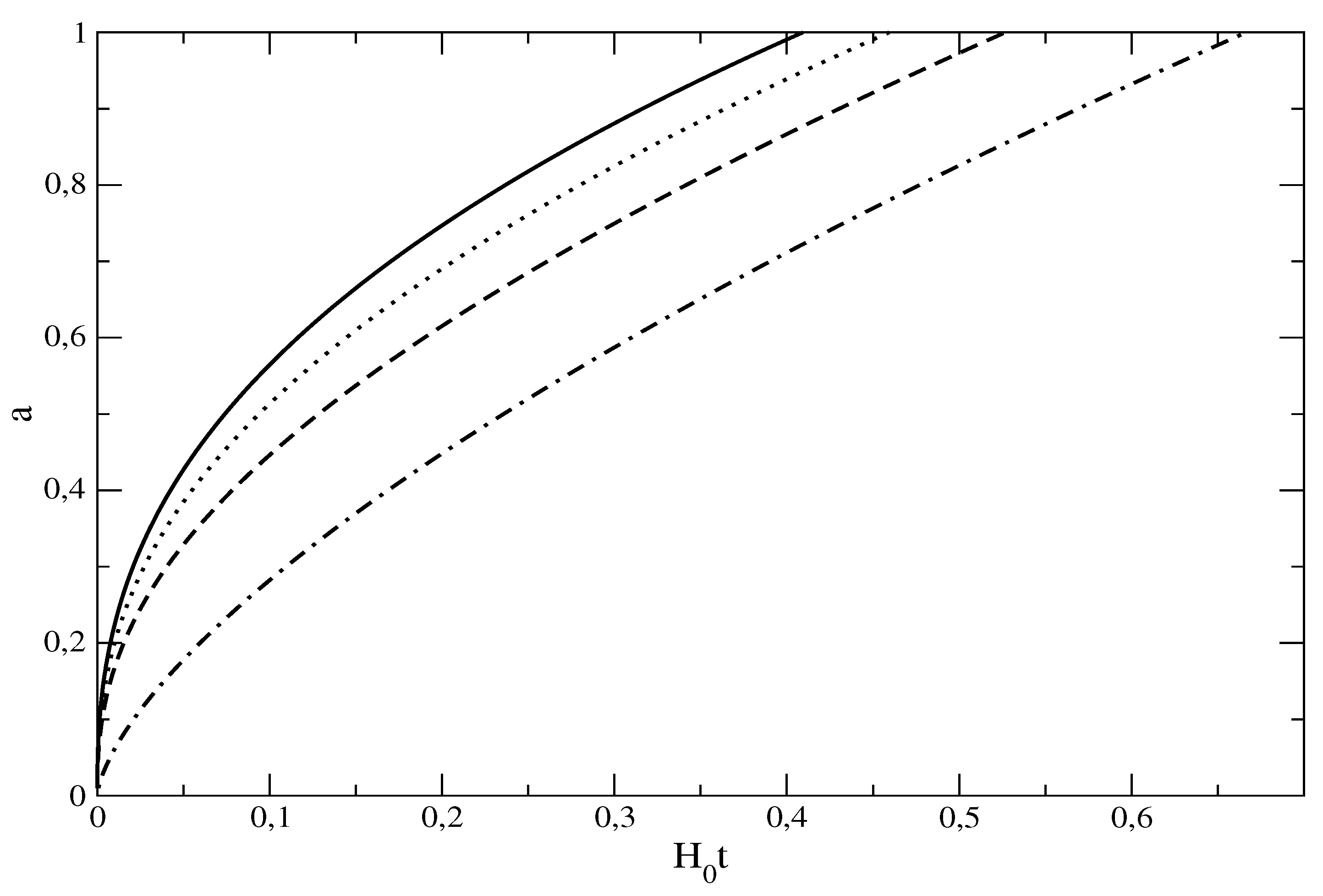
where $H_0$ is the present value of the Hubble parameter, and we have introduced the constants, ${\Omega }_{\mathrm{m}}=8\pi G{M}_0/3H_0^2$, ${\Omega }_{\mathrm{p}}=4\pi G{p}_0/H_0^2$ and ${\Omega }_{\Lambda }=\Lambda /3H_0^2$. Note that we have by definition that ${\Omega }_{\mathrm{m}}+{\Omega }_{\mathrm{p}}+{\Omega }_{\Lambda }=1$. Even without LIVE, this leads to an elliptic integral; so, we have solved this equation numerically. The results in the case, ${\Omega }_{\Lambda }=0$, are shown in Figure 1.

Figure 1. Variation of the scale factor with time for the ideal gas universe model of Section 2, with vanishing cosmological constant, for different values of ${\Omega }_{\mathrm{m}}$ and ${\Omega }_{\mathrm{p}}=1-{\Omega }_{\mathrm{m}}$: ${\Omega }_{\mathrm{m}}=0.1$ (full line), ${\Omega }_{\mathrm{m}}=0.5$ (dotted line), ${\Omega }_{\mathrm{m}}=0.8$ (dashed line) and ${\Omega }_{\mathrm{m}}=1$ (dot-dashed line).

Figure 1. Variation of the scale factor with time for the ideal gas universe model of Section 2, with vanishing cosmological constant, for different values of ${\Omega }_{\mathrm{m}}$ and ${\Omega }_{\mathrm{p}}=1-{\Omega }_{\mathrm{m}}$: ${\Omega }_{\mathrm{m}}=0.1$ (full line), ${\Omega }_{\mathrm{m}}=0.5$ (dotted line), ${\Omega }_{\mathrm{m}}=0.8$ (dashed line) and ${\Omega }_{\mathrm{m}}=1$ (dot-dashed line).

The entropy of the gas is given by the Sackur-Tetrode equation [8], which here takes the form:

$$S=K_1+K_{2}ln\left(a^{2}T\right)$$

(14)

where $K_1$ and $K_2$ are constants. It follows from this equation and Equation (9) that the entropy of a cosmic ideal gas in an expanding homogeneous universe is constant, independently of the other contents of the universe, as long as there is no exchange of energy between the gas and the other ingredients of the universe. The way that the scale factor depends upon time does not matter in this respect.

The constancy of the entropy of the ideal gas is not surprising. In a homogeneous universe, there are no global temperature differences and, hence, no heat for a non-interacting gas. It follows that the expansion is adiabatic and that the entropy of the cosmic gas is constant.

3. Measures of Gravitational Entropy

Since we do not have a theory of quantum gravity, the entropy of the gravitational field cannot be calculated by counting its microstates. In an effort to incorporate the tendency of (attractive) gravity to produce inhomogeneities—and in the most extreme cases, black holes—into a generalized second law of thermodynamics, Penrose [9] made some suggestions about how to define a quantity representing the entropy of a gravitational field. Such a quantity should vanish in the case of a homogeneous field and obtain a maximal value given by the Bekenstein-Hawking entropy for the field of a black hole. In this connection, Penrose formulated what is called the Weyl curvature conjecture, saying that the Weyl curvature should be small, near the initial singularity of the Universe. Wainwright and Anderson [10] interpreted this hypothesis in terms of the ratio of the Weyl and Ricci curvature invariants:

$$P_{\mathrm{WA}}^2=\frac{W_{\alpha \beta \gamma \delta }{W}^{\alpha \beta \gamma \delta }}{R_{\mu \nu }{R}^{\mu \nu }}$$

(15)

According to their formulation of the Weyl curvature hypothesis, $P_{\mathrm{WA}}$ should vanish at the initial singularity of the Universe. The physical content of the hypothesis is that the initial state of the Universe is homogeneous and isotropic. Hence, the hypothesis need not be interpreted as a hypothesis about gravitational entropy. Neither need it refer to an unphysical initial singularity, but should instead be concerned with an initial state, say, at the Planck time.

However, it was shown by Grøn and Hervik [11,12] that according to Einstein’s classical field equations, $P_{\mathrm{WA}}^2$, essentially due to its local nature, diverges at the initial singularity, both in the case of the homogeneous, but anisotropic, Bianchi type I universe models and the isotropic, but inhomogeneous, LTB universe models. This means that there are large anisotropies and inhomogeneities near the initial singularities in these universe models. Hence, the classical behavior is not in agreement with the Weyl curvature conjecture, as formulated in terms of Equation (15).

If the entropy represents a large number of gravitational microstates corresponding to a certain gravitational field, it may be more properly represented by a non-local quantity proportional to $P_{\mathrm{WA}}$. Such a quantity may be finite at the initial singularity, even if $P_{\mathrm{WA}}$ diverges. Grøn and Hervik [11,12] therefore considered the quantity:

$$S_{\mathrm{G}1}=\int k_{\mathrm{S}}{P}_{\mathrm{WA}}dV,dV=\sqrt{g_{11}{g}_{22}{g}_{33}}{d}^{3}x$$

(16)

Here, $k_{\mathrm{S}}$ is a constant, $g_{ii}$ are the spatial components of the metric and V is the invariant volume corresponding to a unit coordinate volume in coordinates co-moving with the cosmic fluid. It was shown in [11,12] that $S_{\mathrm{G}1}$ behaves in accordance with the Weyl curvature conjecture in the LTB models. However, $S_{\mathrm{G}1}$ diverges in the Schwarzschild spacetime, and so, it cannot reproduce the Bekenstein-Hawking entropy of a Schwarzschild black hole. Rudjord, Grøn and Hervik [13], therefore, suggested another definition of gravitational entropy. Considering the spacetime of a black hole, they defined a gravitational entropy current vector through the relation:

$$\overrightarrow{\Psi }=P{\overrightarrow{e}}_{\widehat{r}}$$

(17)

where $P^2$ is a quantity proportional to the Weyl curvature invariant. However, it cannot be given by Equation (15), since the Ricci curvature invariant vanishes in the Schwarzschild spacetime. Therefore, in [13], this expression was replaced by:

$$P^2=\frac{W^{\alpha \beta \gamma \delta }{W}_{\alpha \beta \gamma \delta }}{R^{\alpha \beta \gamma \delta }{R}_{\alpha \beta \gamma \delta }}$$

(18)

where the denominator is the Kretschmann curvature scalar. They proved that $P^2<1$ in all spacetimes with vanishing energy flux, a class that encompasses the spacetime outside the most general Kerr-Newman black hole and the isotropic and homogeneous Friedmann universe models. The entropy of a black hole is proportional to the area of the event horizon. Hence, the entropy can be written as a surface integral over the horizon, σ:

$$S_{\mathrm{G}2}=k_{\mathrm{S}}{\int }_{\sigma }\overrightarrow{\Psi }·d\sigma$$

(19)

and the constant, $k_{\mathrm{S}}$, is determined by demanding that the formula reproduces the Bekenstein-Hawking result for a Schwarzschild black hole, which results in $k_{\mathrm{S}}=k{c}^3{\left(4G\hslash \right)}^{-1}$, where k is Boltzmann’s constant. This means that according to this prescription, all of the entropy of a Schwarzschild black hole is due to the inhomogeneity of the gravitational field. An expression for the entropy density can be found by rewriting Equation (19) as a volume integral by means of the divergence theorem:

$$s=k_{\mathrm{S}}|\nabla ·\overrightarrow{\Psi }|$$

(20)

In the following, we will consider both the definition of gravitational entropy in Equation (16) and the one provided by Equations (17)–(19).

4. Gravitational Entropy in the Plane-Symmetric Bianchi Type I Universe

The line element of the LIVE-dominated, plane symmetric Bianchi type I universe is [14]:

$$d{s}^2=-c^{2}d{t}^2+R_i^2{\left(d{x}^i\right)}^2,i=1,2,3$$

(21)

where:

$$R_1=R_2=2^{2/3}{sinh}^{2/3}\tau ,R_3=2^{2/3}coth\tau {cosh}^{2/3}\tau ,\tau =\frac{1}{2}{(3\Lambda )}^{1/2}t$$

(22)

The comoving volume is:

$$V=sinh\left(2\tau \right)$$

(23)

For this spacetime, the Ricci scalar, the Weyl scalar and the Kretschmann curvature scalar are, respectively:

$$R_{\mu \nu }{R}^{\mu \nu }=36H_0^2,W_{\mu \nu \alpha \beta }{W}^{\mu \nu \alpha \beta }=\frac{12H_0^2}{{sinh}^4\tau },R_{\mu \nu \alpha \beta }{R}^{\mu \nu \alpha \beta }=24H_0^2+\frac{12H_0^2}{{sinh}^4\tau }$$

(24)

Hence, the quantities, $P_{\mathrm{WA}}$ and P are, respectively:

$$P_{\mathrm{WA}}=\frac{1}{\sqrt{3}{sinh}^2\tau },P=\frac{1}{\sqrt{1+2{sinh}^4\tau }}$$

(25)

This gives

$$S_{\mathrm{G}1}=\frac{k_{\mathrm{S}}}{\sqrt{3}}coth\tau ,S_{\mathrm{G}2}=k_{\mathrm{S}}\frac{sinh\tau cosh\tau }{\sqrt{1+2{sinh}^4\tau }}$$

(26)

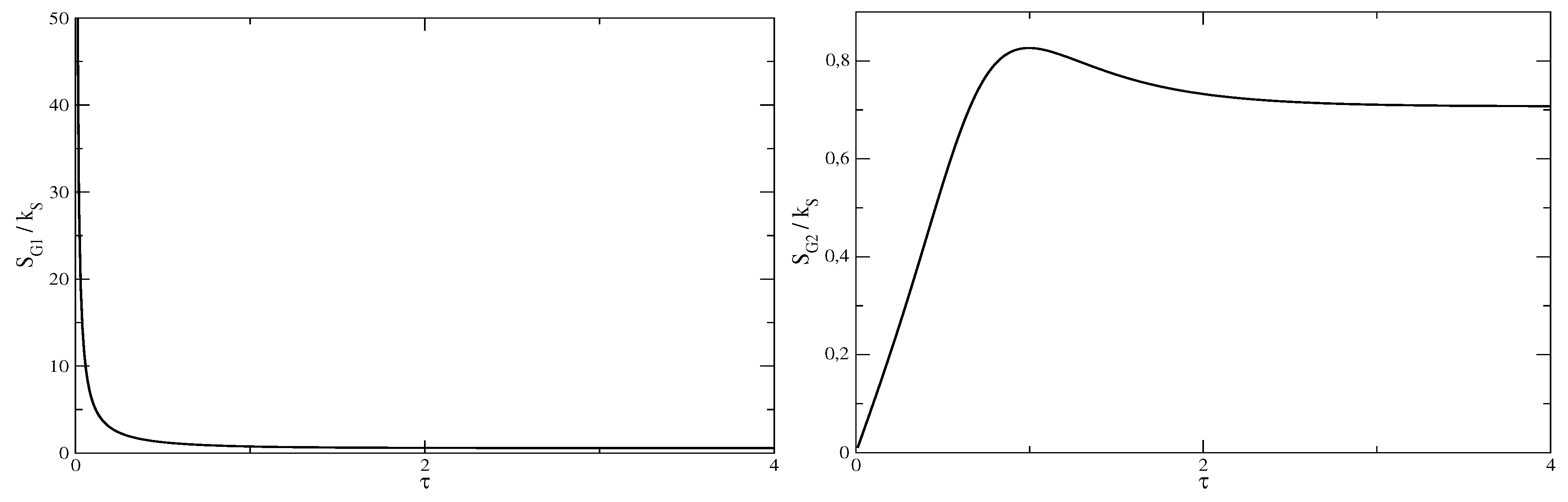
The time variations of these quantities at the beginning of the inflationary era are shown in Figure 2. We see that if $S_{\mathrm{G}1}$ or $S_{\mathrm{G}2}$ were a dominating form of entropy, then the entropy of the Universe decreased during most of the part of the inflationary era, except possibly during a transient initial period.

Figure 2. Time variation of the candidate gravitational entropies, $S_{\mathrm{G}1}$ (left panel) and $S_{\mathrm{G}2}$ (right panel), in a comoving volume during the beginning of the inflationary era.

Figure 2. Time variation of the candidate gravitational entropies, $S_{\mathrm{G}1}$ (left panel) and $S_{\mathrm{G}2}$ (right panel), in a comoving volume during the beginning of the inflationary era.

5. Gravitational Entropy in LTB Models with LIVE

We next turn our attention to inhomogeneous cosmological models described by the Lemaitre-Tolman-Bondi (LTB) line element:

$$d{s}^2=-d{t}^2+X^2(r,t)d{r}^2+R^2(r,t)d{\Omega }^2$$

(27)

where $d{\Omega }^2=d{\theta }^2+{sin}^2\theta d{\varphi }^2$. We follow [15] and consider a spherically symmetric energy-momentum tensor:

$$T_{\nu }^{\mu }=\mathrm{diag}(-\rho \left(r\right)-{\rho }_{\mathrm{m}}(r,t),p_r\left(r\right),p_t\left(r\right),p_t\left(r\right))$$

(28)

Here, ${\rho }_{\mathrm{m}}(r,t)$ is the density of pressureless matter, and the dark energy is represented by the density, $\rho \left(r\right)$, and the radial and transverse pressures, $p_r\left(r\right)$ and ${\rho }_r\left(r\right)$. In [15], it was shown that the Einstein equations imply:

$$H^2(r,t)=H_0^2\left(r\right)\left[{\Omega }_{\mathrm{m}}\left(r\right){\left(\frac{R_0}{R}\right)}^3+{\Omega }_{\mathrm{D}}\left(r\right)+{\Omega }_k\left(r\right){\left(\frac{R_0}{R}\right)}^2\right]$$

(29)

with:

$$H(r,t)=\frac{\dot{R}(r,t)}{R(r,t)}$$

(30)

$R_0\left(r\right)=R(r,t_0)$, $t_0$ being the present epoch, $H_0\left(r\right)=H(r,t_0)$, ${\Omega }_{\mathrm{D}}\left(r\right)=-8\pi G{p}_r\left(r\right){\left[3H_0^2\left(r\right)\right]}^{-1}$ and ${\Omega }_k\left(r\right)=1-{\Omega }_{\mathrm{m}}\left(r\right)-{\Omega }_{\mathrm{D}}\left(r\right)$. We will consider models with ${\Omega }_{\mathrm{m}}\left(r\right)=0={\Omega }_k\left(r\right)$ in order to mimic inflation. In this case, ${\Omega }_{\mathrm{D}}\left(r\right)=1$, which gives:

$$p_r\left(r\right)=-\frac{3H_0^2\left(r\right)}{8\pi G}$$

(31)

The Einstein equations then give the following simple equation for R:

$$\frac{\dot{R}}{R}=H_0\left(r\right)$$

(32)

with solutions of the form:

$$R(r,t)=R_0\left(r\right)e^{H_0\left(r\right)(t-t_0)}$$

(33)

The function, X, is determined by the condition, $X(r,t)=R^{\prime }(r,t)$, which also follows from the Einstein equations. The functions, $R_0\left(r\right)$ and $H_0\left(r\right)$, are arbitrary.

Since a definition of gravitational entropy should reproduce the Bekenstein-Hawking entropy of a Schwarzschild black hole, we choose to show results for the entropy, $S_{\mathrm{G}2}$, defined in Equation (19). Calculating the Weyl and Kretschmann invariants analytically is a cumbersome task and the resulting expressions not very illuminating, so this was done numerically from the components of the Riemann tensor.

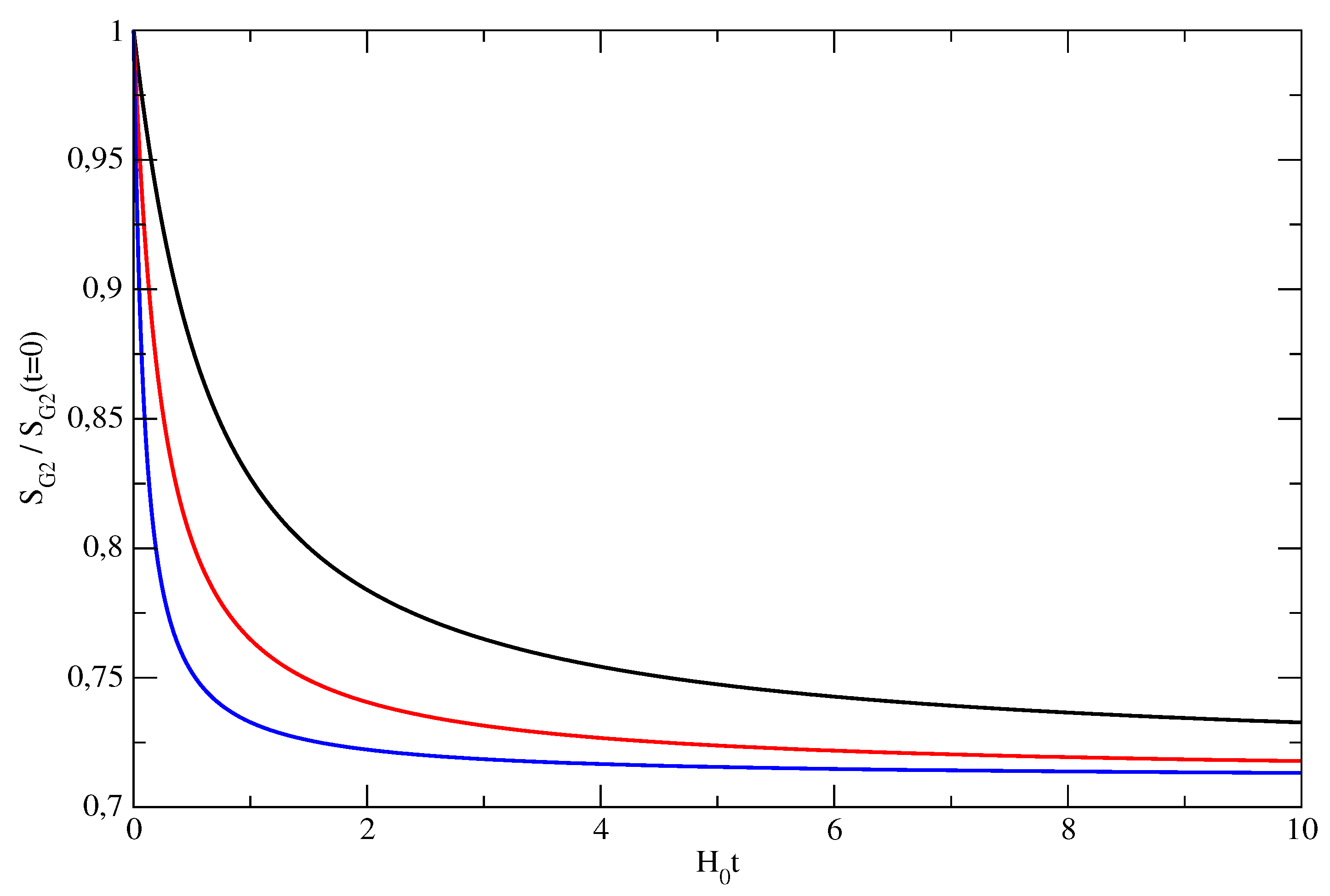
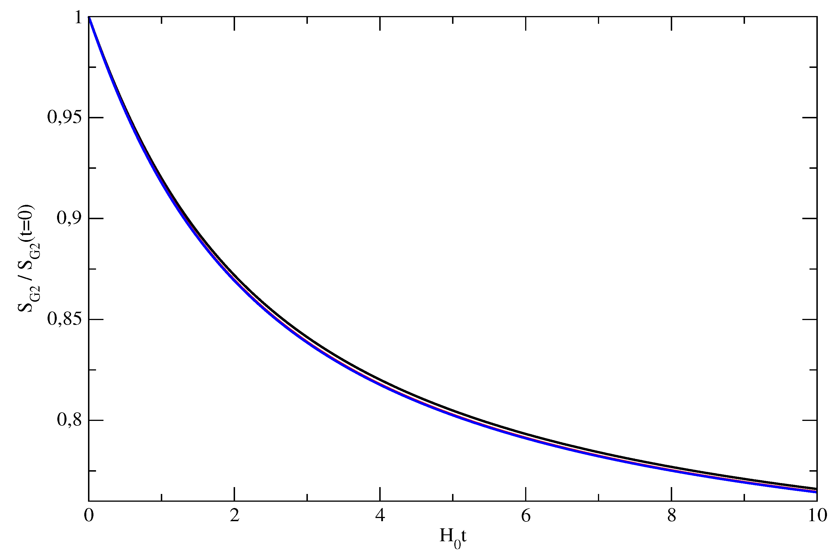
In Figure 3, we have plotted the time evolution of the entropy within spheres of different comoving radii. We have chosen $H_0\left(r\right)=H_{c}cosh(r/r_0)$, $R_0\left(r\right)=R_{c}sinh(r/r_0)$, where $H_c$, $R_c$ and $r_0$ are constants. If we choose instead $H_0\left(r\right)=H_{c}tanh(r/r_0)$, $R_0\left(r\right)=R_{c}tanh(r/r_0)$, we get the results shown in Figure 4 for the evolution of the entropy. In both cases, we see that the gravitational entropy, $S_{\mathrm{G}2}$, decreases rapidly in the beginning and, then, flattens out at later times. With this definition of gravitational entropy, we see that also in this model, as in the case of the Bianchi type I model of the previous section, the gravitational entropy is decreased by inflation.

Figure 3. The variation with time, relative to the initial value, of the total gravitational entropy within spheres of varying radius.The black curve corresponds to $r=2r_0$, the red curve to $r=3r_0$ and the blue curve to $r=4r_0$. Here, $H_0\left(r\right)=H_{c}cosh(r/r_0)$, $R_0\left(r\right)=R_{c}sinh(r/r_0)$.

Figure 3. The variation with time, relative to the initial value, of the total gravitational entropy within spheres of varying radius.The black curve corresponds to $r=2r_0$, the red curve to $r=3r_0$ and the blue curve to $r=4r_0$. Here, $H_0\left(r\right)=H_{c}cosh(r/r_0)$, $R_0\left(r\right)=R_{c}sinh(r/r_0)$.

Figure 4. The variation with time, relative to the initial value, of the total gravitational entropy within spheres of varying radius. The black curve corresponds to $r=2r_0$, the red curve to $r=3r_0$ and the blue curve to $r=4r_0$. Here, $H_0\left(r\right)=H_{c}tanh(r/r_0)$, $R_0\left(r\right)=R_{c}tanh(r/r_0)$.

Figure 4. The variation with time, relative to the initial value, of the total gravitational entropy within spheres of varying radius. The black curve corresponds to $r=2r_0$, the red curve to $r=3r_0$ and the blue curve to $r=4r_0$. Here, $H_0\left(r\right)=H_{c}tanh(r/r_0)$, $R_0\left(r\right)=R_{c}tanh(r/r_0)$.

6. A Model of Entropy Generation at the End of the Inflationary Era

A. Bonanno and M. Reuter [5,6,7] have investigated a new mechanism of entropy generation during the inflationary era. The physics behind their model is associated with the renormalization group and results in possible variations of the density of vacuum energy as represented by a time-varying cosmological “constant”, $\Lambda \left(t\right)$, and a varying gravitational “constant”, $G\left(t\right)$.

According to their model, the time variation of G is much smaller than that of Λ, and will be neglected here. Additionally, in the present work, we shall specifically consider a transformation of vacuum energy to radiation energy at the end of the inflationary era.

Following Bonanno and Reuter [7], the modified Friedmann equation and the continuity equation for a spatially flat universe have the forms:

$$\begin{array}{ccc}\hfill H^2& =& \frac{8\pi G}{3}\rho +\frac{\Lambda \left(t\right)}{3}\hfill \end{array}$$

(34)

$$\begin{array}{ccc}\hfill \dot{\rho }+4H\rho & =& -\frac{\dot{\Lambda }}{8\pi G}\hfill \end{array}$$

(35)

where ρ is the density of radiation, and the time variation of the density of the vacuum energy is given in terms of the Hubble parameter by:

$$\Lambda \left(t\right)={\Lambda }_0\left[1+{\left(\frac{H}{H_T}\right)}^4\right]$$

(36)

where $H_T$ is a constant.

From Equations (34) and (35), it follows that:

$$\dot{H}=-\frac{16\pi }{3}G\rho$$

(37)

Hence, we must have $\dot{H}<0$ in order to have the density of radiation, $\rho >0$. From Equation (34), it follows that:

$$\frac{8\pi G}{3H^2}\rho +\frac{\Lambda \left(t\right)}{3H^2}\equiv \Omega +{\Omega }_{\Lambda }=1$$

(38)

and from Equation (36), we have:

$${\Omega }_{\Lambda }=H_{\Lambda }^2\left(\frac{1}{H^2}+\frac{H^2}{H_T^4}\right)$$

(39)

with $H_{\Lambda }\equiv \sqrt{{\Lambda }_0/3}$.

Taking time derivatives of Equation (36) and Equation (37) and substituting in Equation (35), we find:

$$3\ddot{H}+12H\dot{H}=\frac{8{\Lambda }_0}{H_T^4}{H}^3\dot{H}$$

(40)

which can readily be integrated once, with respect to time, to give:

$$\dot{H}+2H^2=\frac{2H_{\Lambda }^2}{H_T^4}{H}^4+2C$$

(41)

where C is a constant of integration. From this result and Equation (37), we get:

$$\Omega =-\frac{\dot{H}}{H^2}=1-\frac{H_{\Lambda }^2}{H_T^4}{H}^2-\frac{C}{H^2}$$

(42)

and from Equation (39), we find:

$$\Omega +{\Omega }_{\Lambda }=1+\frac{H_{\Lambda }^2-C}{H^2}$$

(43)

Therefore, to satisfy the condition (38), we must choose $C=H_{\Lambda }^2$. Then, Equation (41) becomes:

$$\dot{H}=2\left(\frac{H_{\Lambda }^2}{H_T^4}{H}^4-H^2+H_{\Lambda }^2\right)=\frac{2H_{\Lambda }^2}{H_T^4}(H^2-H_1^2)(H^2-H_2^2)$$

(44)

where:

$$H_{1,2}^2=\frac{H_T^4}{2H_{\Lambda }^2}\left(1\pm \sqrt{1-\frac{4H_{\Lambda }^4}{H_T^4}}\right)$$

(45)

We must have $H_T>\sqrt{2}{H}_{\Lambda }$ to have real solutions, and in that case, $H_1>H_2>0$. Additionally, to ensure that $\dot{H}<0$, so that the radiation energy density is positive, the Hubble parameter must be in the interval, $H_2<H<H_1$. The general solution of Equation (44) can then be written as:

$${\left(\frac{H_1-H}{H_1+H}\right)}^{H_2}{\left(\frac{H+H_2}{H-H_2}\right)}^{H_1}=Kexp\left\{4H_{\Lambda }{\left[{\left(\frac{H_T}{H_{\Lambda }}\right)}^4-4\right]}^{1/2}t\right\}$$

(46)

with

$$K={\left(\frac{H_1-H_0}{H_1+H_0}\right)}^{H_2}{\left(\frac{H_0+H_2}{H_0-H_2}\right)}^{H_1}$$

(47)

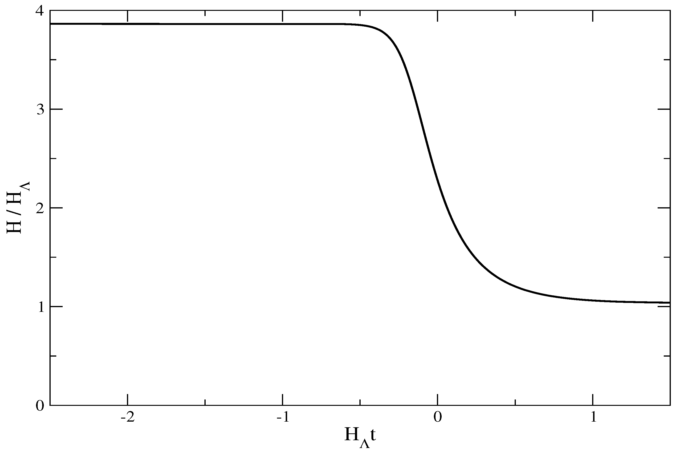
where $H_0=H\left(0\right)$. Note that ${lim}_{t\to \infty }H=H_2$, ${lim}_{t\to -\infty }H=H_1$ and $H_1>H_2$. The graph of H as a function of $H_{\Lambda }t$ is shown in Figure 5.

Figure 5. The variation with time of the Hubble parameter in the model of Section 6.

Figure 5. The variation with time of the Hubble parameter in the model of Section 6.

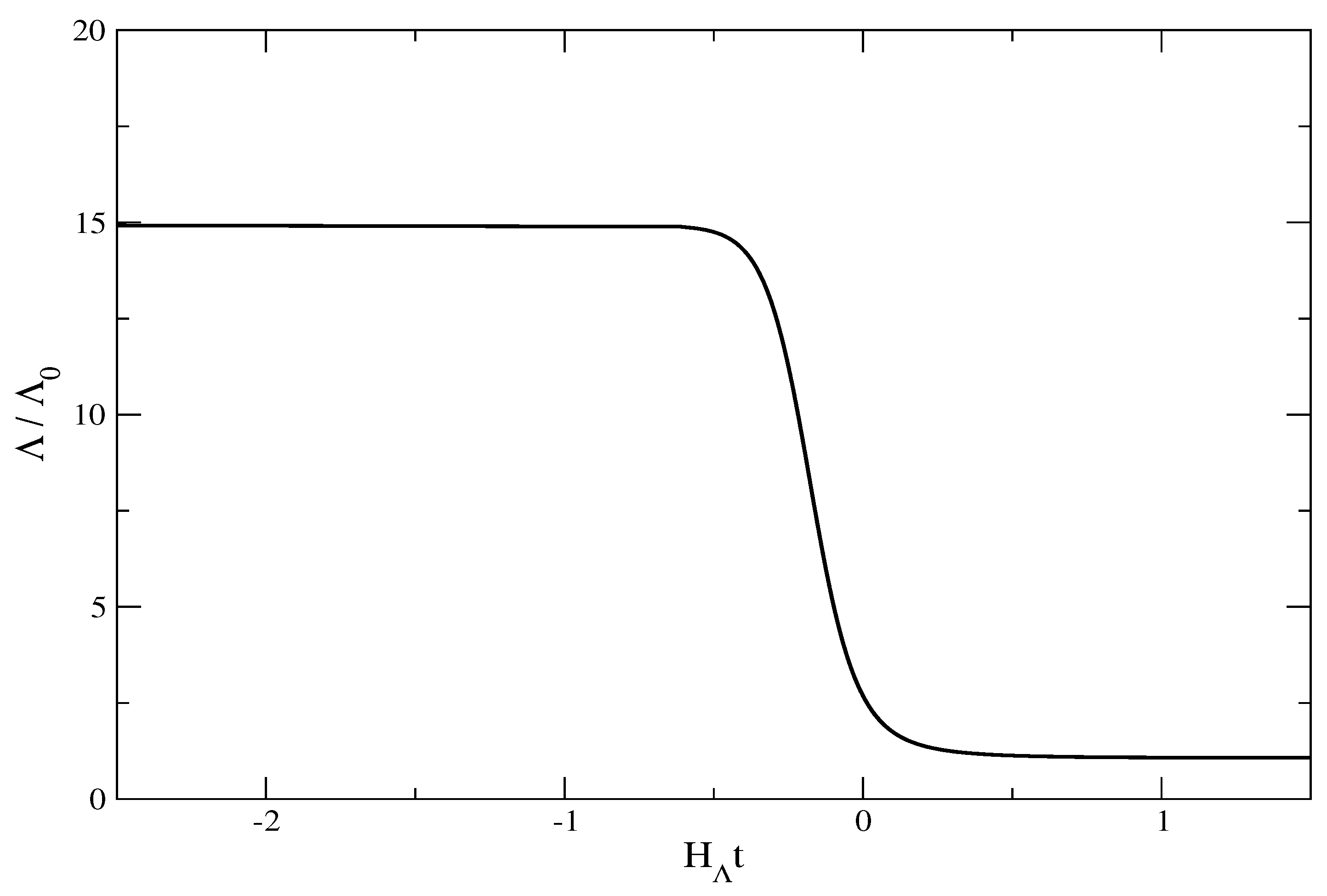
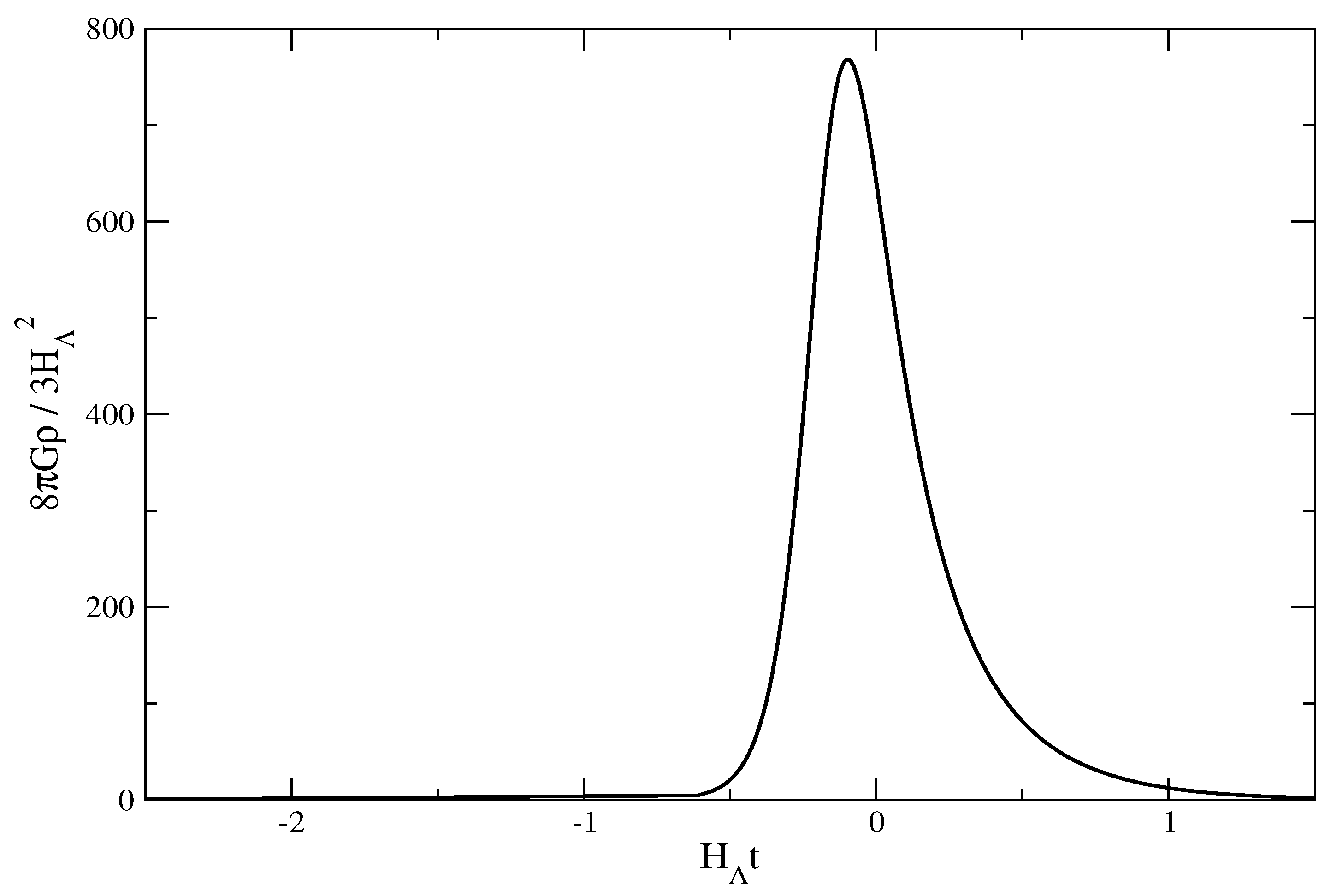
In Figure 6, $\Lambda /{\Lambda }_0$, given by Equation (36), is plotted as a function of τ. The density of the radiation can be found, e.g., from Equation (38), and is plotted in Figure 7. From Equations (37) and (40), it follows that the radiation density has a maximum for $H=H_T^2/\sqrt{2}{H}_{\Lambda }$. Inserting this in Equation (34) gives the maximum radiation density:

$${\rho }_{\max }=\frac{3H_{\Lambda }^2}{8\pi G}\left[\frac{1}{4}{\left(\frac{H_T}{H_{\Lambda }}\right)}^4-1\right]$$

(48)

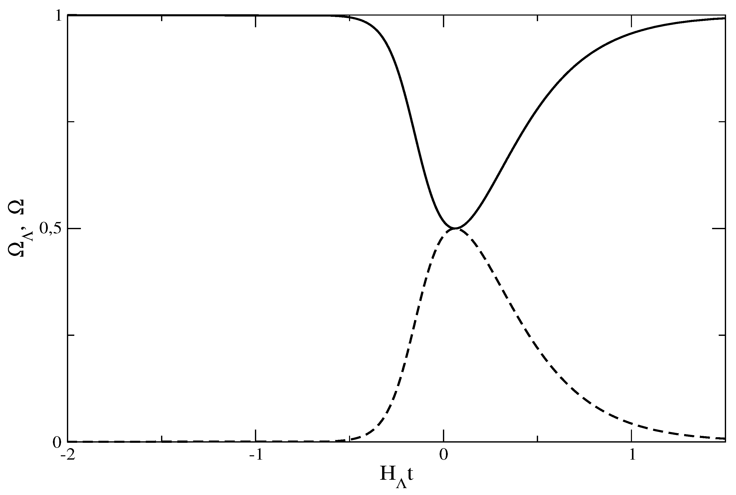
The maximum value of the density parameter of the radiation and the corresponding minimum value of the density parameter of the vacuum energy are, respectively:

$${\Omega }_{\max }=1-2{\left(\frac{H_{\Lambda }}{H_T}\right)}^2,{\Omega }_{\Lambda ,\min }=2{\left(\frac{H_{\Lambda }}{H_T}\right)}^2$$

(49)

Figure 6. The variation with time of $\Lambda /{\Lambda }_0$ in the model of Section 6.

Figure 6. The variation with time of $\Lambda /{\Lambda }_0$ in the model of Section 6.

Figure 7. The variation with time of the radiation energy density in the model of Section 6.

Figure 7. The variation with time of the radiation energy density in the model of Section 6.

Figure 8. The variation with time of the vacuum energy density parameter, ${\Omega }_{\Lambda }$, (full line), and the density parameter for radiation, Ω, (dashed line) in the model of Section 6.

Figure 8. The variation with time of the vacuum energy density parameter, ${\Omega }_{\Lambda }$, (full line), and the density parameter for radiation, Ω, (dashed line) in the model of Section 6.

Figure 8 shows the evolution of the density parameters, Ω and ${\Omega }_{\Lambda }$.

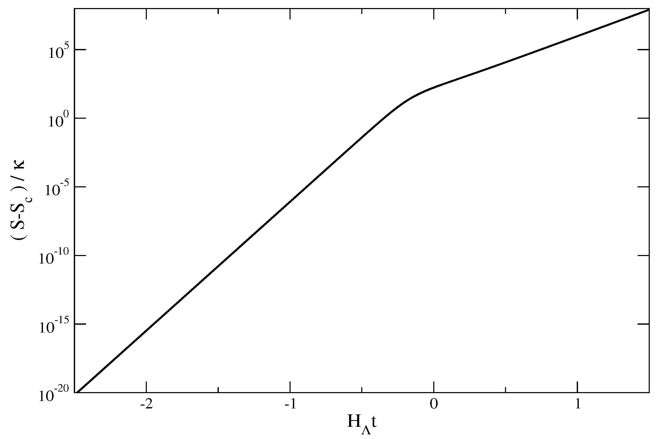
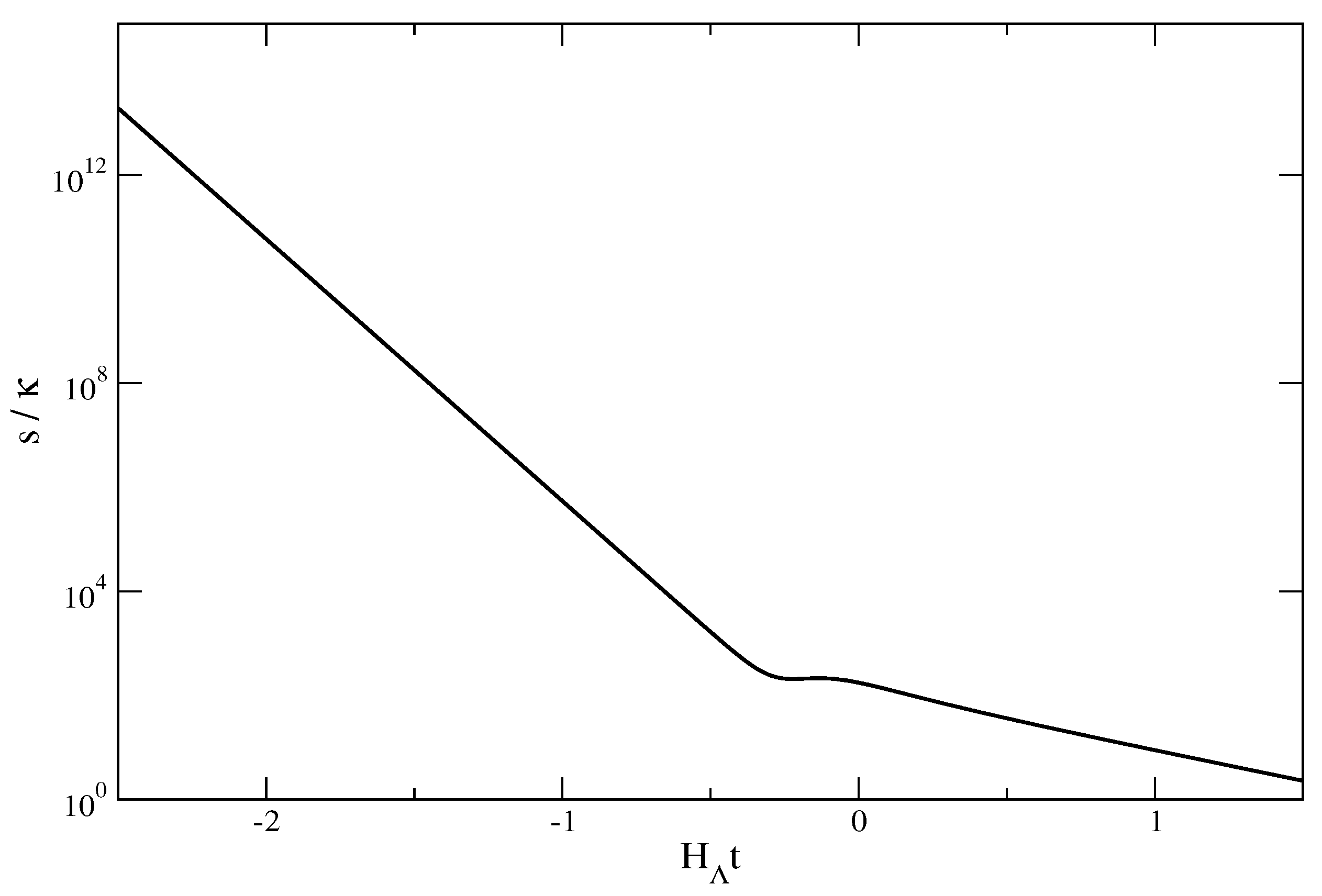
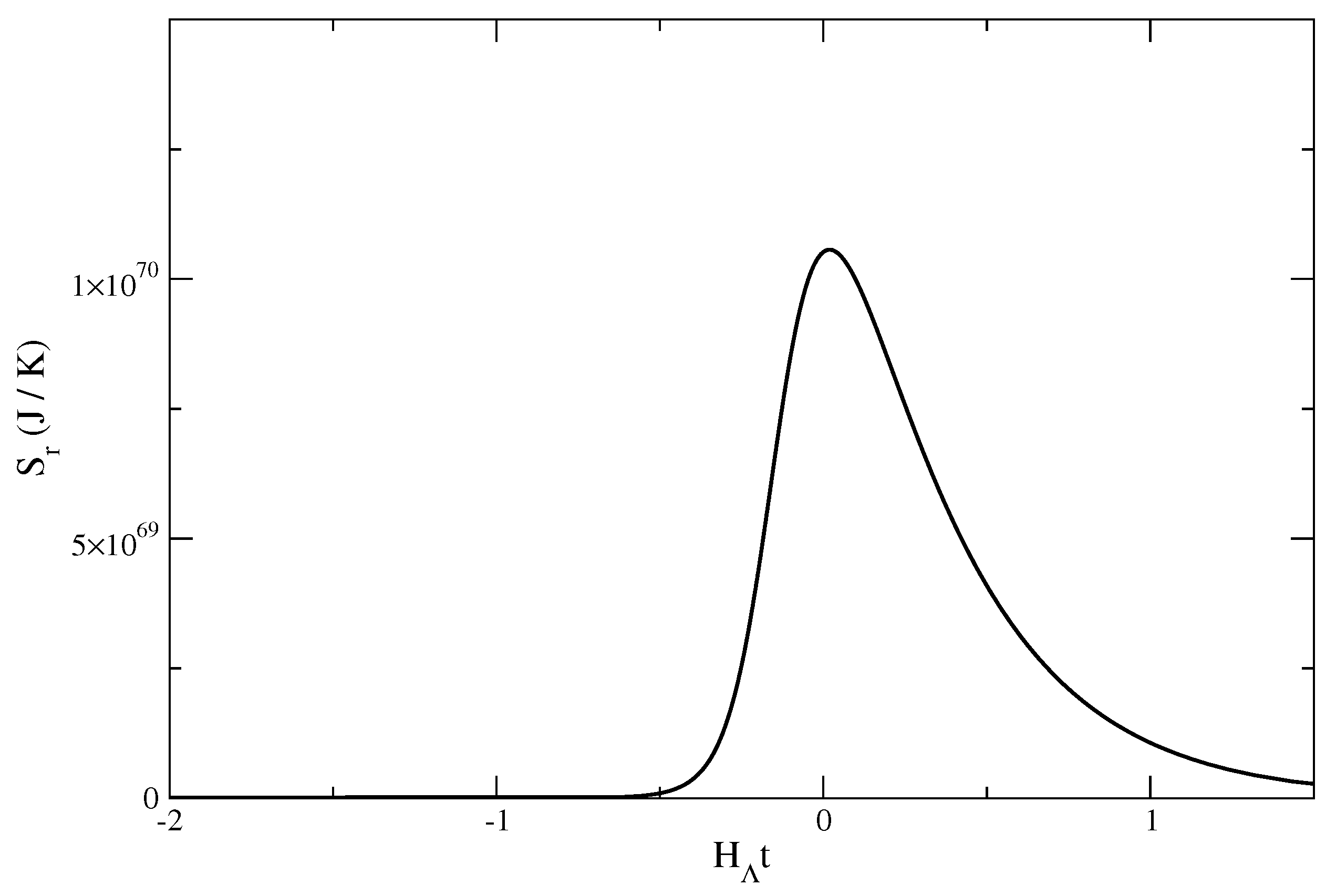
As shown in [7], the entropy of the radiation in a comoving volume is given by:

$$S\left(t\right)=\frac{4}{3}\kappa a^3{\rho }^{3/4}+S_c$$

(50)

and the entropy density by:

$$s\left(t\right)=\frac{4}{3}\kappa {\rho }^{3/4}+\frac{S_c}{a^3}$$

(51)

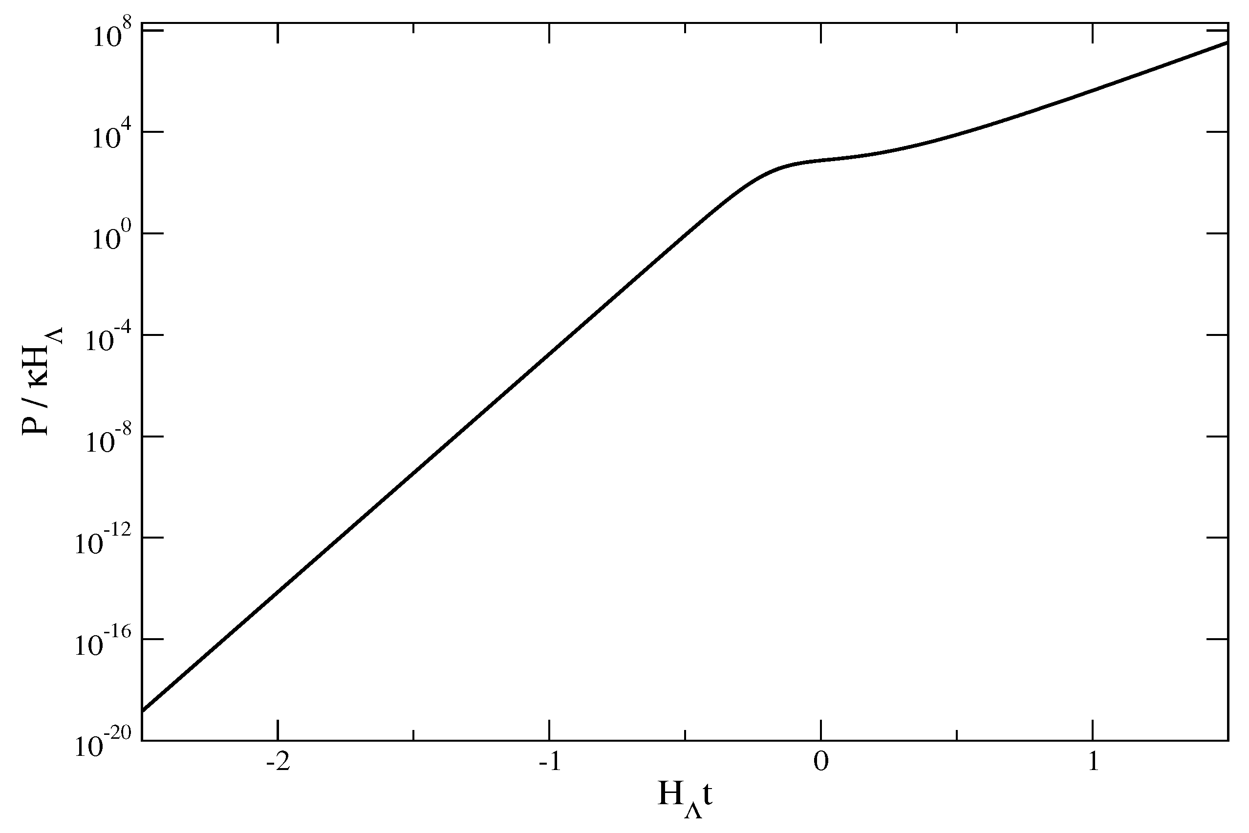
where κ is a constant. These functions are plotted in Figure 9 and Figure 10. In the case of a universe with non-interacting LIVE and radiation, the density of the radiation decreases as $\rho \propto a^{-4}$. Then, $a^3{\rho }^{3/4}=$ constant. In such a universe, the entropy of radiation in a comoving volume is constant. Finally, the entropy production rate, $P\left(t\right)=\dot{S\left(t\right)}$, can, from Equations (16) and (18) in [7], be written as:

$$P\left(t\right)=-\frac{a^3\dot{\Lambda }}{8\pi GT}=-\frac{\kappa a^3\dot{\Lambda }}{8\pi G{\rho }^{1/4}}.$$

(52)

Taking the time derivative of Equation (36) and using Equation (37), $\dot{\Lambda =-64\pi {\Lambda }_{0}G{H}^3\rho /3H_T^4}$; so, the entropy production rate is given by:

$$P\left(t\right)=\frac{8\kappa {\Lambda }_0{\left(aH\right)}^3{\rho }^{3/4}}{3H_T^4}=\frac{2\kappa {\Lambda }_0}{H_T^4}{H}^3(S-S_c).$$

(53)

This quantity is plotted in Figure 11.

Figure 9. The variation with time of the entropy in the model of Section 6.

Figure 9. The variation with time of the entropy in the model of Section 6.

Figure 10. The variation with time of the entropy density in the model of Section 6.

Figure 10. The variation with time of the entropy density in the model of Section 6.

Figure 11. The variation with time of the entropy production in the model of Section 6.

Figure 11. The variation with time of the entropy production in the model of Section 6.

7. The Concept of a Maximal Entropy for the Universe

There are several conjectures as to what the maximal entropy of the Universe may be [16]. One is the so-called Bekenstein bound [17]. According to this, the maximum entropy of a system with radius R and non-gravitational energy E is:

$$S_{\mathrm{Max}-\mathrm{Bek}}=2\pi \frac{k_B}{\hslash c}RE$$

(54)

The physical meaning is that the entropy lost into a black hole cannot be larger than the increase in the horizon entropy of the black hole. In the context of a flat FRWuniverse, the Bekenstein bound says that the maximal entropy inside a comoving surface with standard coordinate radius χ is:

$$S_{\mathrm{Max}-\mathrm{Bek}}=\frac{8{\pi }^2}{3}\frac{k_B}{\hslash c}{\chi }^4\rho a^4$$

(55)

For a universe dominated by a cosmic fluid with equation of state $p=w\rho$, the density changes during the expansion according to $\rho a^{3(1+w)}={\rho }_0$, where ${\rho }_0$ is the present density. Hence, the Bekenstein bound for the cosmic entropy is proportional to $a^{1-3w}$. In the radiation-dominated phase that lasted for about the first fifty thousand years after the Big Bang, the dominating fluid, i.e., the radiation, had $w=1/3$. Hence, the Bekenstein maximum of entropy was constant during the radiation-dominated era. For cosmic matter with $w<1/3$, for example, cold dark matter with $w=0$, the Bekenstein bound increases with time, and for cosmic dark energy with $w<-1$, the Bekenstein bound increases faster than in the matter-dominated era.

Secondly, the Holographic bound [18,19] may be formulated by asserting that for a given volume, V, the state of maximal entropy is the one containing the largest black hole that fits inside V, and this maximum is given by the finite area that encloses this volume. As applied to the space inside the cosmological horizon in a FRW universe, this gives the entropy bound:

$$S_{\mathrm{Max}-\mathrm{Hol}}=\pi k_B{\left(\frac{\chi a}{{\ell }_P}\right)}^2$$

(56)

where ${\ell }_P$ is the Planck length. In the present era of our Universe, which is becoming more and more dominated by dark energy, possibly in the form of LIVE, the holographic bound (56) increases exponentially fast in the future. Several versions of this bound have been discussed by Custadio and Horvath [20].

Frautschi [21] identified the maximum entropy inside the particle horizon of a universe as the entropy that is produced if all matter inside the horizon collapses to a single black hole. Again, as applied to a flat FRW universe, this leads to:

$$S_{\mathrm{Max}-\mathrm{Fra}}=\frac{64{\pi }^3{k}_{B}G}{9\hslash c}{\left({\chi }_{\mathrm{PH}}^3\rho a^3\right)}^2$$

(57)

For a universe dominated by a cosmic fluid with equation of state $p=w\rho$, this implies that $S_{\mathrm{Max}-\mathrm{Fra}}\propto a^{-3w}$. Hence, an era dominated by cold matter has approximately constant value for this upper bound on the entropy. The bound decreased in the radiation-dominated era, and it increases in the present and future dark energy-dominated era. However, this bound is ill-defined for the model of this section, since the scale factor behaves like $a\sim exp\left(H_{1}t\right)$ as $t\to -\infty$, and hence, there is no particle horizon.

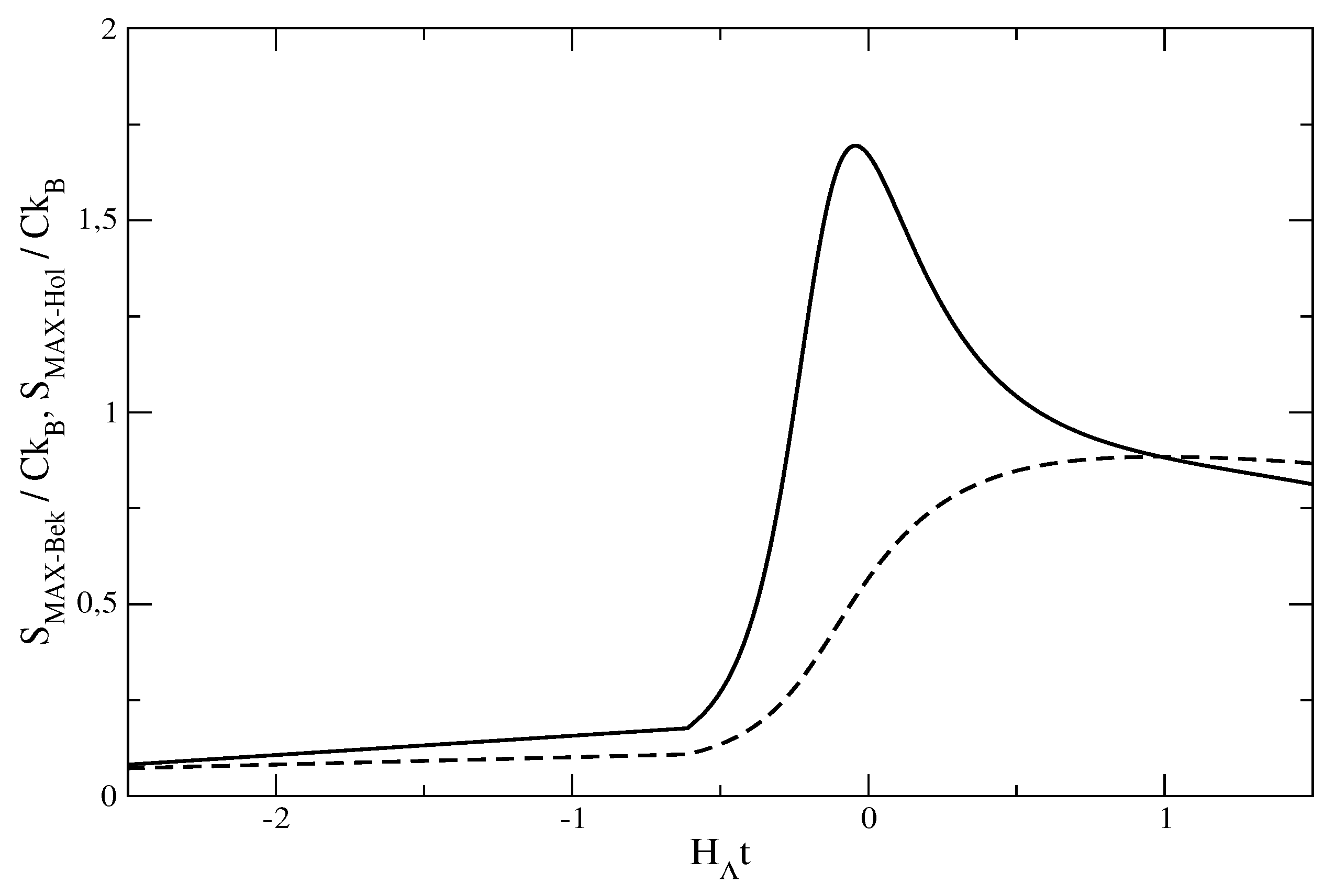
As applied to our description of the transition of vacuum energy to radiation energy at the end of the inflationary era, these proposals for the maximal entropy of the Universe give time variations of the maximal entropy, as shown in Figure 12. In Figure 13, we show the radiation entropy contained within the event horizon. The figures show that a gap opens up between the radiation entropy and all the entropy bounds and that the former is insignificant in comparison with the latter.

Figure 12. The Bekenstein (full line) and holographic (dashed line) upper bounds on the entropy of the universe as functions of time in the model of Section 6. The entropy is plotted in units of Boltzmann’s constant and have also been divided by a factor, $C=1.0295\times {10}^{122}$.

Figure 12. The Bekenstein (full line) and holographic (dashed line) upper bounds on the entropy of the universe as functions of time in the model of Section 6. The entropy is plotted in units of Boltzmann’s constant and have also been divided by a factor, $C=1.0295\times {10}^{122}$.

Figure 13. The radiation entropy contained within the event horizon as a function of time in the model of Section 6. Note that it is miniscule compared to the entropy bounds in the previous figures.

Figure 13. The radiation entropy contained within the event horizon as a function of time in the model of Section 6. Note that it is miniscule compared to the entropy bounds in the previous figures.

8. Entropy Gap and the Arrow of Time

P. C. W. Davis has summarized some main concepts related to the term “the arrow of time” in his Whithrow lecture [22]. Already, in 1854, Helmholtz introduced the term “the heat death of the universe” as a consequence of the second law of thermodynamics, which had recently been formulated. It says that the entropy of a closed system can never decrease. Since the Universe may be considered to be the supreme closed system, it follows that the entropy of the Universe cannot decrease. The final state is one of thermodynamic equilibrium, where nothing of the thermal energy in the Universe can be utilized to perform work. This is the heat death of the Universe.

On the other hand, the entropy of the Universe must have been smaller earlier in the history of the Universe than it is today. However, measurements of the temperature variations in the cosmic microwave background radiation show that the radiation was in a state of nearly thermal equilibrium with maximal thermal entropy, already 400,000 years after the Big Bang.

If the Universe contained LIVE, cold matter in the form of dust with practically zero temperature, and radiation, the dominating contribution to the thermal entropy of the Universe would come from the radiation, and the Universe was then in a state of maximal entropy at early times.

Assume now that there were two components contributing significantly to the thermal entropy of the Universe: an ideal gas and radiation. According to Equation (9), the temperature of the ideal gas depends on the scale factor as $T\propto a^{-2}$. The temperature of the radiation, on the other hand, varies with the scale factor as $T\propto a^{-1}$. Hence, even if the gas and the radiation had the same temperature at some early point in time, the expansion of the Universe would force the temperature of the gas and the radiation to evolve away from each other. There could then exist a cosmic heat engine acting between the gas and the radiation, producing useful work. Then, the thermal entropy of the Universe would be a decreasing function of time. If there is no other form of entropy, this would be in conflict with the second law of thermodynamics, unless one defined such a two-component universe as an open system, which we consider rather artificial.

A solution of this difficulty is to postulate that there must exist other types of entropy than the thermal one, and the sum of the entropies must have been much less than the maximal value at early periods in the history of the Universe.

A classic article discussing the concept of maximal entropy in an expanding universe and the significance of an entropy gap between the actual entropy of the Universe and the maximal entropy for the cosmic arrow of time is that of Frautschi [21]. He introduced the concept of a causal region in the Universe and defined the maximal entropy in the causal region as the entropy of a black hole made of the mass in the region. He then calculated the time evolution of the maximal entropy and the actual entropy in an expanding universe and showed how an entropy gap opens up between the maximal entropy and the actual entropy.

This has also been discussed by Penrose [9,23], who has estimated the gap quantitatively. He found that the maximum possible value of the entropy of the Universe at a given point in time can be taken to be the entropy of a black hole made up of the mass inside the cosmic event horizon at that time. This leads to a maximal entropy on the order of magnitude $S_{max}\approx {10}^{123}{k}_B$ at present. On the other hand, the thermal entropy of the radiation inside the horizon is on the order of $S\approx {10}^{90}{k}_B$. Hence, at the present time, there is a large entropy gap between the actual entropy of the Universe and the maximum possible entropy.

For a gravitating system, homogeneity means low entropy, and inhomogeneity with the matter collected in black holes means large entropy. The large entropy gap means that the Universe is in a very homogeneous state compared to a state where most of the matter is collected in black holes. This requires an explanation.

The most probable reason according to our present understanding is to be found in the extremely early inflationary era, which lasted for ∼${10}^{-33}$ s. In this era, gravity was repulsive, and the Universe evolved towards homogeneity. That is how an immensely large entropy gap opened up.

After the inflationary era, gravity became attractive, and the further entropic evolution of the Universe was to try to close the entropy gap. This gives a direction for the evolution of the Universe—an arrow of time.

More recently, Aquilano, Castagnino and Eiroa [24] have discussed the future evolution of the entropy gap due to conversion of gravitational and kinetic energy in stars. They found that the most significant process in this connection is the production of radiation in the photospheres of stars.

9. Conclusions

We have investigated the generation of entropy in different scenarios with matter, radiation and vacuum energy. Three types of entropy have been considered: thermal entropy related to the internal energy of a gas, gravitational entropy related to the inhomogeneity of a gravitational field, as represented by the Weyl curvature tensor, and horizon entropy, which originated from the relativistic theory of the thermodynamics of black holes. We have considered at least one example of each type.

There is no thermal entropy associated with dust, but a monoatomic ideal gas has a thermal entropy given by the Sackur-Tetrode equation. As shown in Section 2, the thermal entropy of a non-interacting ideal gas in a comoving volume remains constant during the expansion of the Universe.

The time evolution of the gravitational entropy of the Weyl type has been calculated for a plane-symmetric Bianchi type I universe model and two examples of the class of LTB universe models. In both cases, we found that the gravitational entropy associated with the global gravitational field in these universes was decreasing during the expansion. This is as expected. The Weyl entropy is expected to be of relevance mostly in connection with the increasing inhomogeneity of the mass distribution on a more local scale [25].

Finally, we have given a further development of a universe model presented by Bonanno and Reuter [5,6,7], which allows for the transition of vacuum energy to radiation energy. We have calculated the time evolution of several quantities at the end of the inflationary era for this model. During this brief period, the Hubble parameter changes from a nearly constant high value to a much lower value, as shown in Figure 5. The evolution of the density of the vacuum energy, shown in Figure 6, decreases in a similar way as the Hubble parameter, which is to be expected, since a vacuum dominated universe has constant Hubble parameter and a constant density of vacuum energy. The variation with time of the radiation energy density is shown in Figure 7. First, it increases, due to a rapid transition of vacuum energy to radiation; then, it decreases, due to the expansion of the Universe and the slowing down of the vacuum energy-radiation transition. Figure 9 and Figure 10 show that although the entropy density of the radiation decreases with time due to the expansion, the thermal entropy in a comoving volume increases, and Figure 11 shows that there is a steady entropy production. This is due to the conversion of vacuum energy to radiation energy. Figure 12 shows the time evolution of the Bekenstein and holographic upper bounds on the entropy of the Universe at the end of the inflationary era, and Figure 13 shows the thermal radiation entropy within the horizon during this period. Note that this entropy varies in a different way from the radiation entropy in a comoving volume, since the horizon is not a comoving surface. The radiation entropy inside the horizon reaches a maximum value and, then, starts decreasing. Hence, an entropy gap opens up between the actual entropy of the Universe and the maximum possible entropy. This imposes a thermodynamic arrow of time upon the Universe.

References

- Davies, P.C.W. Inflation and the time asymmetry in the Universe. Nature 1983, 301, 398–400. [Google Scholar]
- Veneziano, G. Entropy bounds and string cosmology. High Energy Phys.—Theory 1999. arXiv: hep-th/9907012. [Google Scholar]
- Page, D.N. Inflation does not explain time asymmetry. Nature 1983, 304, 39–41. [Google Scholar] [CrossRef]
- Davies, P.C.W. Inflation in the universe and time asymmetry. Nature 1984, 312, 524–527. [Google Scholar] [CrossRef]
- Bonanno, A.; Reuter, M. Cosmology with self-adjusting vacuum energy density from a renormalization group fixed point. Phys. Lett. B 2002, 527, 9–17. [Google Scholar] [CrossRef] [Green Version]
- Bonanno, A.; Reuter, M. Entropy signature of the running cosmological constant. J. Cosmol. Astropart. Phys. 2007. [Google Scholar] [CrossRef]
- Bonanno, A.; Reuter, M. Entropy production during asymptotically safe inflation. Entropy 2011, 13, 274–292. [Google Scholar] [CrossRef]
- Wallace, D. Gravity, entropy and cosmology: In search of clarity. Br. J. Philos. Sci. 2010, 61, 513–540. [Google Scholar] [CrossRef]
- Penrose, R. Singularities and Time Asymmetry. In General Relativity, an Einstein Centenary Survey; Hawking, S.W., Israel, W., Eds.; Cambridge University Press: New York, NY, USA, 1979; pp. 581–638. [Google Scholar]
- Wainwright, J.; Anderson, P.J. Isotropic singularities and isotropization in a clas of Bianchi type VIh cosmologies. Gen. Rel. Grav. 1984, 16, 609–624. [Google Scholar]
- Grøn, Ø.; Hervik, S. Gravitational entropy and quantum cosmology. Class. Quant. Grav. 2001, 18, 601–618. [Google Scholar] [CrossRef]
- Grøn, Ø.; Hervik, S. The weyl curvature conjecture. Int. J. Theor. Phys. Group Theory Nonlinear Opt. 2003, 10, 29–51. [Google Scholar]
- Rudjord, Ø.; Grøn, Ø.; Hervik, S. The weyl curvature conjecture and black hole entropy. Phys. Scr. 2008, 77, 1–7. [Google Scholar] [CrossRef]
- Grøn, Ø. Expansion isotropization during the inflationary era. Phys. Rev. D 1985, 32, 2522–2527. [Google Scholar] [CrossRef]
- Grande, J.; Perivolaropoulos, L. Generalized LTB model with inhomogeneous isotropic dark energy: Observational constraints. Phys. Rev. D 2011, 84, 023514. [Google Scholar] [CrossRef]
- Grøn, Ø. Entropy and gravity. Entropy 2012, 14, 2456–2477. [Google Scholar] [CrossRef]
- Bekenstein, J.D. Universal upper bound to entropy-to-energy ratio for bounded systems. Phys. Rev. D 1981, 23, 287–298. [Google Scholar] [CrossRef]
- T’ Hooft, G. Dimensional reduction in quantum gravity. Gen. Relativ. Quantum Cosmol. 2009. arXiv:gr-qc/9310026. [Google Scholar]
- Susskind, L. The world as a hologram. J. Math. Phys 1995, 36, 6377–6396. [Google Scholar] [CrossRef]
- Custadio, P.S.; Horvath, J.E. Supermassive black holes may be limited by the holographic bound. Gen. Rel. Grav. 2003, 35, 1337–1349. [Google Scholar] [CrossRef]
- Frautschi, S. Entropy in an expanding universe. Science 1982, 217, 593–599. [Google Scholar] [CrossRef] [PubMed]
- Davies, P.C.W. The arrow of time. Astron. Geophys. 2005, 46, 1.26–1.29. [Google Scholar] [CrossRef]
- Penrose, R. The Road to Reality; Jonathan Cape: London, UK, 2004. [Google Scholar]
- Aquilano, R.; Castagnino, M.; Eiroa, E. Entropy gap and time asymmetry II. Mod. Phys. Lett. 2000, A15, 875–882. [Google Scholar] [CrossRef]
- Amarzguioui, M.; Grøn, Ø. Entropy of gravitationally collapsing matter in FRW universe models. Phys. Rev. D 2005, 71, 083001. [Google Scholar] [CrossRef]
© 2013 by the authors; licensee MDPI, Basel, Switzerland. This article is an open access article distributed under the terms and conditions of the Creative Commons Attribution license (http://creativecommons.org/licenses/by/3.0/).
Share and Cite
MDPI and ACS Style
Elgarøy, Ø.; Grøn, Ø. Gravitational Entropy and Inflation. Entropy 2013, 15, 3620-3639. https://0-doi-org.brum.beds.ac.uk/10.3390/e15093620
AMA Style
Elgarøy Ø, Grøn Ø. Gravitational Entropy and Inflation. Entropy. 2013; 15(9):3620-3639. https://0-doi-org.brum.beds.ac.uk/10.3390/e15093620
Chicago/Turabian StyleElgarøy, Øystein, and Øyvind Grøn. 2013. "Gravitational Entropy and Inflation" Entropy 15, no. 9: 3620-3639. https://0-doi-org.brum.beds.ac.uk/10.3390/e15093620