Theoretical Foundations and Mathematical Formalism of the Power-Law Tailed Statistical Distributions

Abstract

We present the main features of the mathematical theory generated by the κ-deformed exponential function ${exp}_{\kappa }\left(x\right)={(\sqrt{1+{\kappa }^2{x}^2}+\kappa x)}^{1/\kappa }$, with $0\le \kappa <1$, developed in the last twelve years, which turns out to be a continuous one parameter deformation of the ordinary mathematics generated by the Euler exponential function. The κ-mathematics has its roots in special relativity and furnishes the theoretical foundations of the κ-statistical mechanics predicting power law tailed statistical distributions, which have been observed experimentally in many physical, natural and artificial systems. After introducing the κ-algebra, we present the associated κ-differential and κ-integral calculus. Then, we obtain the corresponding κ-exponential and κ-logarithm functions and give the κ-version of the main functions of the ordinary mathematics.

1. Introduction

Undoubtedly the most interesting feature of the statistical distribution function:

$$f_i={exp}_{\kappa }(-\beta E_i+\beta \mu )$$

(1)

where the κ-exponential is defined as:

$${exp}_{\kappa }\left(x\right)={(\sqrt{1+{\kappa }^2{x}^2}+\kappa x)}^{1/\kappa },0\le \kappa <1$$

(2)

is represented by its asymptotic behavior, namely:

$$f_i\genfrac{}{}{0pt}{}{}{\stackrel{\sim }{\beta E_i-\beta \mu \to 0}}exp(-\beta E_i+\beta \mu ),f_i\genfrac{}{}{0pt}{}{}{\stackrel{\sim }{E_i\to +\infty }}N{E}_i^{-1/\kappa }$$

(3)

The above κ-distribution at low energies is the ordinary Boltzmann distribution, while at high energies, it presents a power-law tail. For this reason, the statistical theory [1,2,3,4,5,6,7,8,9,10], based on the distribution in Equation (1), has attracted the interest of many researchers.

In the last twelve years, various authors have considered the foundations of the statistical theory based on the κ-distribution, in connection with the historical evolution of the research on the power-law tailed statistical distributions [7,11], e.g., the H-theorem and the molecular chaos hypothesis [12,13], the thermodynamic stability [14,15], the Lesche stability [16,17,18,19], the Legendre structure of the ensued thermodynamics [20,21], the thermodynamics of non-equilibrium systems [22], quantum versions of the theory [23,24,25,26], the geometrical structure of the theory [27], various mathematical aspects of the theory [3,28,29,30,31,32,33,34,35], etc. On the other hand, specific applications to physical systems have been considered, e.g., cosmic rays [6], relativistic [37] and classical [38] plasmas in the presence of external electromagnetic fields, the relaxation in relativistic plasmas under wave-particle interactions [39,40], anomalous diffusion [41,42], non-linear kinetics [43,44,45], kinetics of interacting atoms and photons [46], particle kinetics in the presence of temperature gradients [47,48], particle systems in external conservative force fields [49], stellar distributions in astrophysics [50,51,52,53], quark-gluon plasma formation citeTewel, quantum hadrodynamics models [55], fracture propagation [56], etc. Other applications concern dynamical systems at the edge of chaos [57,58,59], fractal systems [60], field theories [61], random matrix theory [62,63,64], error theory [65], game theory [66], the theory of complex networks [67], information theory [68], etc. Furthermore, applications to economic systems have been considered, e.g., to study personal income distribution [69,70,71,72,73,74], to model deterministic heterogeneity in tastes and product differentiation [75,76], in finance [77,78], in equity options [79], to construct taxation and redistribution models [80], etc.

In this contribution, we present the main features of the mathematical theory generated by the function, ${exp}_{\kappa }\left(x\right)$. The κ-mathematics, developed in the last twelve years, turn out to be a continuous one parameter deformation of the ordinary mathematics generated by the Euler exponential function. The κ-mathematics has its roots in special relativity and furnishes the theoretical foundations of the κ-statistical theory predicting power law tailed statistical distributions, which have been observed experimentally in many physical, natural and artificial systems.

The paper is organized as follows: After introducing the κ-algebra, we present the associated κ-differential and κ-integral calculus. Then, we obtain the corresponding κ-generalized exponential and logarithmic functions and give the κ-version of the main functions of the ordinary mathematics.

2. κ-Algebra

Theorem 1. Let $x,y\in \mathbf{R}$ and $-1<\kappa <1$. The composition law, $\stackrel{\kappa }{\oplus }$, defined through:

$$x\stackrel{\kappa }{\oplus }y=x\sqrt{1+{\kappa }^2{y}^2}+y\sqrt{1+{\kappa }^2{x}^2}$$

(4)

is a generalized sum, called the κ-sum, and the algebraic structure $(\mathbf{R},\stackrel{\kappa }{\oplus })$ forms an abelian group.

Proof. From the definition of $\stackrel{\kappa }{\oplus }$, the following properties follow.

(1)

associativity: $\left(x\stackrel{\kappa }{\oplus }y\right)\stackrel{\kappa }{\oplus }z=x\stackrel{\kappa }{\oplus }\left(y\stackrel{\kappa }{\oplus }z\right)$,

(2)

neutral element: $x\stackrel{\kappa }{\oplus }0=0\stackrel{\kappa }{\oplus }x=x$,

(3)

opposite element: $x\stackrel{\kappa }{\oplus }(-x)=(-x)\stackrel{\kappa }{\oplus }x=0$,

(4)

commutativity: $x\stackrel{\kappa }{\oplus }y=y\stackrel{\kappa }{\oplus }x$.

 

☐

Remark 1. The κ-sum is a one parameter continuous deformation of the ordinary sum, which recovers in the classical limit $\kappa \to 0$, i.e., $x\stackrel{0}{\oplus }y=x+y$. The κ-sum in Equation (4) is the additivity law of the dimensionless relativistic momenta of special relativity, while the real parameter $-1<\kappa <1$ is the reciprocal of the dimensionless light speed [3,9]. The κ-difference $\stackrel{\kappa }{\ominus }$ is defined as $x\stackrel{\kappa }{\ominus }y=x\stackrel{\kappa }{\oplus }(-y)$.

Theorem 2. Let $x,y\in \mathbf{R}$ and $-1<\kappa <1$. The composition law, $\stackrel{\kappa }{\otimes }$, defined through:

$$x\stackrel{\kappa }{\otimes }y=\frac{1}{\kappa }sinh\left(\frac{1}{\kappa }\mathrm{arcsinh}\left(\kappa x\right)\mathrm{arcsinh}\left(\kappa y\right)\right)$$

(5)

is a generalized product, called the κ-product, and the algebraic structure $(\mathbf{R},\stackrel{\kappa }{\otimes })$ forms an abelian group.

Proof. From the definition of $\stackrel{\kappa }{\otimes }$, the following properties follow.

(1)

associativity: $\left(x\stackrel{\kappa }{\otimes }y\right)\stackrel{\kappa }{\otimes }z=x\stackrel{\kappa }{\otimes }\left(y\stackrel{\kappa }{\otimes }z\right)$,

(2)

neutral element: is defined through $x\stackrel{\kappa }{\otimes }I=I\stackrel{\kappa }{\otimes }x=x$ and is given by $I={\kappa }^{-1}sinh\kappa$,

(3)

inverse element: is defined through $x\stackrel{\kappa }{\otimes }\overline{x}=\overline{x}\stackrel{\kappa }{\otimes }x=I$ and is given by $\overline{x}={\kappa }^{-1}sinh({\kappa }^2/\mathrm{arcsinh}\kappa x)$,

(4)

commutativity: $x\stackrel{\kappa }{\otimes }y=y\stackrel{\kappa }{\otimes }x$.

 

☐

Remark 2. The κ-product reduces to the ordinary product as $\kappa \to 0$, i.e., $x\stackrel{0}{\otimes }y=xy$. The κ-division $\stackrel{\kappa }{\oslash }$ is defined through $x\stackrel{\kappa }{\oslash }y=x\stackrel{\kappa }{\otimes }\overline{y}$.

Theorem 3. Let $x,y\in \mathbf{R}$ and $-1<\kappa <1$. The κ-sum $\stackrel{\kappa }{\oplus }$ defined in Equation (4) and the κ-product $\stackrel{\kappa }{\otimes }$ defined in Equation (5) obey the distributive law:

$$z\stackrel{\kappa }{\otimes }\left(x\stackrel{\kappa }{\oplus }y\right)=\left(z\stackrel{\kappa }{\otimes }x\right)\stackrel{\kappa }{\oplus }\left(z\stackrel{\kappa }{\otimes }y\right)$$

(6)

and then, the algebraic structure $(\mathbf{R},\stackrel{\kappa }{\oplus },\stackrel{\kappa }{\otimes })$ forms an abelian field.

Proof. The relationship in Equation (6) follows directly from the definitions of the κ-product in Equation (5) and of the κ-sum in Equation (4), which can be written also in the form:

$$x\stackrel{\kappa }{\oplus }y=\frac{1}{\kappa }sinh\left(\mathrm{arcsinh}\left(\kappa x\right)+\mathrm{arcsinh}\left(\kappa y\right)\right)$$

(7)

 

☐

Theorem 4. The abelian fields, $(\mathbf{R},\stackrel{\kappa }{\oplus },\stackrel{\kappa }{\otimes })$ and $(\mathbf{R},+,.)$, are isomorphic.

Proof. After introducing the function, $\left\{x\right\}\in C^{\infty }\left(\mathbf{R}\right)$, through:

$$\left\{x\right\}=\frac{1}{\kappa }\mathrm{arcsinh}\left(\kappa x\right)$$

(8)

whose inverse function, $\left[x\right]\in C^{\infty }\left(\mathbf{R}\right)$, i.e., $\left[\right\{x\left\}\right]=\left\{\right[x\left]\right\}=x$, is given by:

$$\left[x\right]=\frac{1}{\kappa }sinh\left(\kappa x\right)$$

(9)

we can write Equation (7) and Equation (5) in the form:

$$\begin{array}{ccc}& & \left\{x\stackrel{\kappa }{\oplus }y\right\}=\left\{x\right\}+\left\{y\right\}\hfill \end{array}$$

(10)

$$\begin{array}{ccc}& & \left\{x\stackrel{\kappa }{\otimes }y\right\}=\left\{x\right\}·\left\{y\right\}\hfill \end{array}$$

(11)

or, equivalently, as:

$$\begin{array}{ccc}& & \left[x\right]\stackrel{\kappa }{\oplus }\left[y\right]=[x+y]\hfill \end{array}$$

(12)

$$\begin{array}{ccc}& & \left[x\right]\stackrel{\kappa }{\otimes }\left[y\right]=[x·y]\hfill \end{array}$$

(13)

 

☐

Theorem 5. Let $x\in \mathbf{R}$ and n be an arbitrary nonnegative integer. It holds:

$$\underset{ntimes}{\underbrace{x\stackrel{\kappa }{\oplus }x\stackrel{\kappa }{\oplus }...\stackrel{\kappa }{\oplus }x}}=\left[n\right]\stackrel{\kappa }{\otimes }x$$

(14)

Proof. The function, $\left[x\right]$, and its inverse, $\left\{x\right\}$, obey the condition $\left[\right\{x\left\}\right]=\left\{\right[x\left]\right\}=x$. Furthermore, we take into account Equation (10) and (13). Then, we have:

$$\begin{array}{ccc}\hfill x\stackrel{\kappa }{\oplus }x\stackrel{\kappa }{\oplus }...\stackrel{\kappa }{\oplus }x& =& \left[\{x\stackrel{\kappa }{\oplus }x\stackrel{\kappa }{\oplus }...\stackrel{\kappa }{\oplus }x\}\right]\hfill \end{array}$$

$$\begin{array}{ccc}& =& \left[\right\{x\}+\{x\}+...+\{x\left\}\right]\hfill \end{array}$$

$$\begin{array}{ccc}\hfill & =& [n·\{x\left\}\right]\hfill \end{array}$$

$$\begin{array}{ccc}\hfill & =& \left[\right\{\left[n\right]\}·\{x\left\}\right]\hfill \end{array}$$

$$\begin{array}{ccc}\hfill & =& \left[n\right]\stackrel{\kappa }{\otimes }\left[\left\{x\right\}\right]\hfill \end{array}$$

$$\begin{array}{ccc}& =& \left[n\right]\stackrel{\kappa }{\otimes }x\hfill \end{array}$$

(15)

 

☐

3. κ-Differential Calculus

3.1. κ-Differential

The κ-differential of x, indicated by $d_{\kappa }x$, is defined through:

$$\begin{array}{c}\hfill (x+dx)\stackrel{\kappa }{\ominus }x=d_{\kappa }x+0\left({\left(dx\right)}^2\right)\end{array}$$

(16)

and results to be:

$$\begin{array}{c}\hfill d_{\kappa }x=\frac{dx}{{\displaystyle \sqrt{1+{\kappa }^2{x}^2}}}\end{array}$$

(17)

In order to better understand the origin of the expression of $d_{\kappa }x$, we recall that the variable, x, is a dimensionless momentum. Then, the quantity $\gamma \left(x\right)=\sqrt{1+{\kappa }^2{x}^2}$ is the Lorentz factor of relativistic physics, in the momentum representation. Therefore, we can write:

$$\begin{array}{c}\hfill d_{\kappa }x=\frac{dx}{\gamma \left(x\right)}\end{array}$$

(18)

Moreover, it holds:

$$\begin{array}{c}\hfill d_{\kappa }x=d\left\{x\right\}=\frac{d\left\{x\right\}}{dx}dx\end{array}$$

(19)

3.2. κ-Derivative

We define the κ-derivative of the function, $f\left(x\right)$, through:

$$\frac{df\left(x\right)}{d_{\kappa }x}=\underset{z\to x}{lim}\frac{f\left(z\right)-f\left(x\right)}{{\displaystyle z\stackrel{\kappa }{\ominus }x}}\approx \underset{dx\to 0}{lim}\frac{f(x+dx)-f\left(x\right)}{{\displaystyle (x+dx)\stackrel{\kappa }{\ominus }x}}$$

(20)

We observe that $df\left(x\right)/d_{\kappa }x$, which reduces to $df\left(x\right)/dx$ as the deformation parameter, $\kappa \to 0$, can be written in the form:

$$\begin{array}{c}\hfill \frac{df\left(x\right)}{d_{\kappa }x}=\sqrt{1+{\kappa }^2{x}^2}\frac{df\left(x\right)}{dx}\end{array}$$

(21)

From the latter relationship, it follows that the κ-derivative obeys the Leibniz’s rules of the ordinary derivative. After introducing the $\gamma \left(x\right)$ Lorentz factor, the κ-derivative can be written also in the form:

$$\begin{array}{c}\hfill \frac{d}{d_{\kappa }x}=\gamma \left(x\right)\frac{d}{dx}\end{array}$$

(22)

3.3. κ-Integral

We define the κ-integral as the inverse operator of the κ-derivative through:

$$\begin{array}{c}\hfill \int d_{\kappa }xf\left(x\right)=\int \frac{dx}{\sqrt{1+{\kappa }^2{x}^2}}f\left(x\right)\end{array}$$

(23)

and note that it is governed by the same rules of the ordinary integral, which recovers when $\kappa \to 0$.

3.4. Connections with Physics

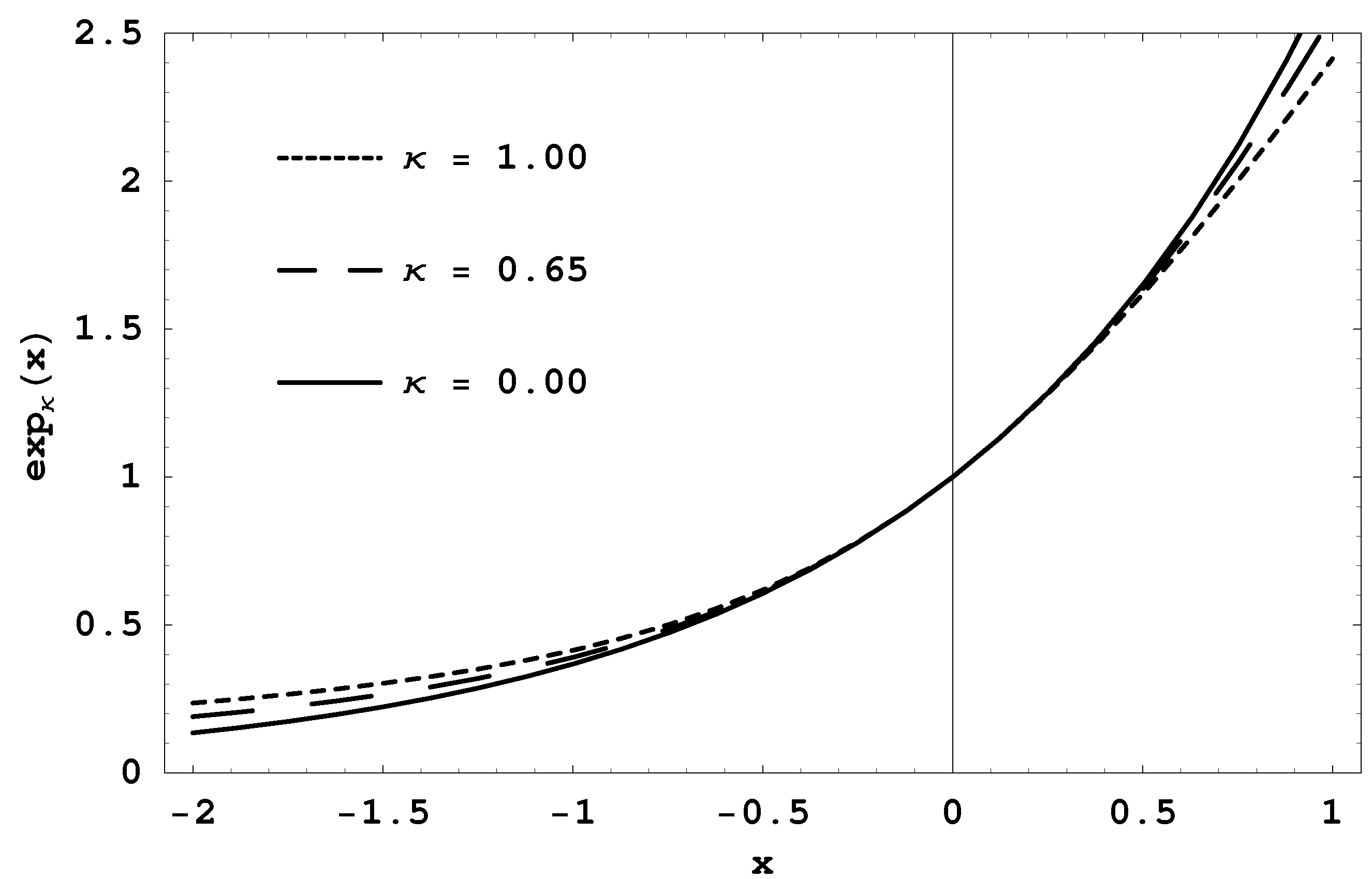
We indicate with $p=\left|\mathbf{p}\right|$ and $x=p/m{v}_{*}$ the moduli of the particle momentum in dimensional and dimensionless form, respectively, and define $\kappa =v_{*}/c$. The classical relationship linking x with the dimensionless kinetic energy $\mathcal{W}=x^2/2$ follows from the kinetic energy theorem, which in differential form reads:

$$\begin{array}{c}\hfill \frac{d}{dx}\mathcal{W}=x\end{array}$$

(24)

The latter equation after replacing the ordinary derivative by the derivative, $d/d_{\kappa }x$, i.e.,:

$$\begin{array}{c}\hfill \frac{d}{d_{\kappa }x}\mathcal{W}=x\end{array}$$

(25)

transforms into the corresponding relativistic equation. This differential equation with the condition $\mathcal{W}(x=0)=0$ admits as a unique solution $\mathcal{W}=\left(\sqrt{1+{\kappa }^2{x}^2}-1\right)/{\kappa }^2$, defining the relativistic kinetic energy.

Let us consider the four-dimensional Lorentz invariant integral:

$$\begin{array}{c}\hfill I=\int d^{4}p\theta \left(p_0\right)\delta (p^{\mu }{p}_{\mu }-m^2{c}^2)F\left(p\right)\end{array}$$

(26)

$p^{\mu }=(p^0,\mathbf{p})=\left(\sqrt{m^2{c}^2+p^2},\mathbf{p}\right)$, $\theta (.)$ being the Heaviside step function and $\delta (.)$, the Dirac delta function. It is trivial to verify that the latter integral transforms into the one-dimension integral:

$$\begin{array}{c}\hfill I\propto \int d_{\kappa }xf\left(x\right)\end{array}$$

(27)

being $f\left(x\right)=4\pi x^{2}F\left(x\right)$. Then, the κ-integral is essentially the Lorentz invariant integral of special relativity.

4. The Function ${exp}_{\kappa }\left(x\right)$

4.1. Definition

We recall that the ordinary exponential $f\left(x\right)=exp\left(x\right)$ emerges as a solution both of the functional equation $f(x+y)=f\left(x\right)f\left(y\right)$ and of the differential equation $(d/dx)f\left(x\right)=f\left(x\right)$. The question to determine the solution of the generalized equations:

$$\begin{array}{c}\hfill f\left(x\stackrel{\kappa }{\oplus }y\right)=f\left(x\right)f\left(y\right)\end{array}$$

(28)

$$\frac{df\left(x\right)}{d_{\kappa }x}=f\left(x\right)$$

(29)

reducing in the $\kappa \to 0$ limit to the ordinary exponential naturally arises. This solution is unique and represents a one-parameter generalization of the ordinary exponential.

Solution of Equation (28): We write this equation explicitly:

$$\begin{array}{c}\hfill f\left(x\sqrt{1+{\kappa }^2{y}^2}+y\sqrt{1+{\kappa }^2{x}^2}\right)=f\left(x\right)f\left(y\right)\end{array}$$

(30)

which, after performing the change of variables, $f\left(x\right)=exp\left(g\right(\kappa x\left)\right)$, $z_1=\kappa x$, $z_2=\kappa y$, transforms as:

$$\begin{array}{c}\hfill g\left(z_1\sqrt{1+z_2^2}+z_2\sqrt{1+z_1^2}\right)=g\left(z_1\right)+g\left(z_2\right)\end{array}$$

(31)

and admits as a solution $g\left(x\right)=A\mathrm{arcsinh}x$. Then, it results that $f\left(x\right)=exp\left(A\mathrm{arcsinh}\kappa x\right)$. The arbitrary constant, A, can be fixed through the condition ${lim}_{\kappa \to 0}f\left(x\right)=exp\left(x\right)$, obtaining $A=1/\kappa$. Therefore, $f\left(x\right)$ assumes the form $f\left(x\right)={exp}_{\kappa }\left(x\right)$, being:

$$\begin{array}{c}\hfill {exp}_{\kappa }\left(x\right)=exp\left(\frac{1}{\kappa }\mathrm{arcsinh}\kappa x\right)\end{array}$$

(32)

Solution of Equation (29): According to Equation (29), the function $f\left(x\right)={exp}_{\kappa }\left(x\right)$ is defined as the eigenfunction of $d/d_{\kappa }x$, i.e.,:

$$\frac{d{exp}_{\kappa }\left(x\right)}{d_{\kappa }x}={exp}_{\kappa }\left(x\right)$$

(33)

After recalling that $d_{\kappa }x=d\left\{x\right\}$ with $\left\{x\right\}={\kappa }^{-1}\mathrm{arcsinh}\kappa x$, Equation (33) can be written in the form:

$$\frac{d{exp}_{\kappa }\left(x\right)}{d\left\{x\right\}}={exp}_{\kappa }\left(x\right)$$

(34)

The solution of the latter equation with the condition ${exp}_{\kappa }\left(0\right)=1$ follows immediately:

$$\begin{array}{c}\hfill {exp}_{\kappa }\left(x\right)=exp\left(\left\{x\right\}\right)\end{array}$$

(35)

After taking into account that $\mathrm{arcsinh}x=ln(\sqrt{1+x^2}+x)$, we can write ${exp}_{\kappa }\left(x\right)$ in the form:

$$\begin{array}{c}\hfill {exp}_{\kappa }\left(x\right)={\left(\sqrt{1+{\kappa }^2{x}^2}+\kappa x\right)}^{1/\kappa }\end{array}$$

(36)

which will be used in the following. We remark that ${exp}_{\kappa }\left(x\right)$ given by Equation (36) is the solution of both Equation (28) and Equation (29) and, therefore, represents a generalization of the ordinary exponential.

4.2. Basic Properties

From the definition in Equation (36) of ${exp}_{\kappa }\left(x\right)$ follows that:

$$\begin{array}{ccc}& & {exp}_0\left(x\right)\equiv \underset{\kappa \to 0}{lim}{exp}_{\kappa }\left(x\right)=exp\left(x\right)\hfill \end{array}$$

(37)

$$\begin{array}{ccc}& & {exp}_{-\kappa }\left(x\right)={exp}_{\kappa }\left(x\right)\hfill \end{array}$$

(38)

Like the ordinary exponential, ${exp}_{\kappa }\left(x\right)$ has the properties:

$$\begin{array}{ccc}& & {exp}_{\kappa }\left(x\right)\in C^{\infty }\left(\mathbf{R}\right)\hfill \end{array}$$

(39)

$$\begin{array}{ccc}& & \frac{d}{dx}{exp}_{\kappa }\left(x\right)>0\hfill \end{array}$$

(40)

$$\begin{array}{ccc}& & {exp}_{\kappa }(-\infty )=0^{+}\hfill \end{array}$$

(41)

$$\begin{array}{ccc}& & {exp}_{\kappa }\left(0\right)=1\hfill \end{array}$$

(42)

$$\begin{array}{ccc}& & {exp}_{\kappa }(+\infty )=+\infty \hfill \end{array}$$

(43)

$$\begin{array}{ccc}& & {exp}_{\kappa }\left(x\right){exp}_{\kappa }(-x)=1\hfill \end{array}$$

(44)

In Figure 1 is plotted the function, ${exp}_{\kappa }\left(x\right)$, defined in Equation (36) for three different values of the parameter of κ. The continuous curve corresponding to $\kappa =0$ is the ordinary exponential function, $exp\left(x\right)$.

Figure 1. Plot of the function, ${exp}_{\kappa }\left(x\right)$, defined in Equation (36) for three different values of the parameter of κ. The continuous curve corresponding to $\kappa =0$ is the ordinary exponential function, $exp\left(x\right)$.

Figure 1. Plot of the function, ${exp}_{\kappa }\left(x\right)$, defined in Equation (36) for three different values of the parameter of κ. The continuous curve corresponding to $\kappa =0$ is the ordinary exponential function, $exp\left(x\right)$.

Property in Equation (44) emerges as a particular case of the more general one:

$$\begin{array}{c}\hfill {exp}_{\kappa }\left(x\right){exp}_{\kappa }\left(y\right)={exp}_{\kappa }\left(x\stackrel{\kappa }{\oplus }y\right)\end{array}$$

(45)

Furthermore, ${exp}_{\kappa }\left(x\right)$ has the property:

$$\begin{array}{ccc}& & {\left({exp}_{\kappa }\left(x\right)\right)}^r={exp}_{\kappa /r}\left(rx\right)\hfill \end{array}$$

(46)

with $r\in \mathbf{R}$, which in the limit, $\kappa \to 0$, reproduces one well known property of the ordinary exponential.

We remark the following convexity property:

$$\begin{array}{c}\hfill \frac{d^2}{d{x}^2}{exp}_{\kappa }\left(x\right)>0;x\in \mathbf{R}\end{array}$$

(47)

holding when ${\kappa }^2<1$.

Undoubtedly, one of the more interesting properties of ${exp}_{\kappa }\left(x\right)$ is its power law asymptotic behavior:

$$\begin{array}{c}\hfill {exp}_{\kappa }\left(x\right)\genfrac{}{}{0pt}{}{}{\stackrel{\sim }{x\to \pm \infty }}|2\kappa x{|}^{\pm 1/\left|\kappa \right|}\end{array}$$

(48)

4.3. Mellin Transform

Let us consider the incomplete Mellin transform of the ${exp}_{\kappa }(-t)$:

$$\begin{array}{ccc}\hfill {\mathcal{M}}_{\kappa }(r,x)& & ={\int }_0^x{t}^{r-1}{exp}_{\kappa }(-t)dt\hfill \end{array}$$

(49)

After performing the change of integration variable $y={\left(\sqrt{1+{\kappa }^2{t}^2}-\left|\kappa \right|t\right)}^2$ and after taking into account that $t=\frac{1}{2\left|\kappa \right|}\left(y^{-1/2}-y^{1/2}\right)$ and ${exp}_{\kappa }(-t)=y^{1/2\left|\kappa \right|}$, the function, ${\mathcal{M}}_{\kappa }(r,x)$, can be written in the form:

$$\begin{array}{ccc}\hfill {\mathcal{M}}_{\kappa }(r,x)& & =\frac{1}{2}{\left|2\kappa \right|}^{-r}{\int }_X^1{y}^{\frac{1}{2\left|\kappa \right|}-\frac{r}{2}-1}{\left(1-y\right)}^{r-1}\left(1+y\right)dy\hfill \end{array}$$

(50)

with:

$$\begin{array}{c}\hfill X={\left(\sqrt{1+{\kappa }^2{x}^2}-\left|\kappa \right|x\right)}^2\end{array}$$

(51)

When r is an integer greater than zero, ${\mathcal{M}}_{\kappa }(r,x)$ can be calculated analytically. For instance, it results:

$$\begin{array}{ccc}& & {\mathcal{M}}_{\kappa }(1,x)=\frac{1}{1-{\kappa }^2}-\frac{{\kappa }^{2}x+\sqrt{1+{\kappa }^2{x}^2}}{1-{\kappa }^2}{exp}_{\kappa }(-x)\hfill \end{array}$$

(52)

$$\begin{array}{ccc}& & {\mathcal{M}}_{\kappa }(2,x)=\frac{1}{1-4{\kappa }^2}-\frac{1+2{\kappa }^2{x}^2+x\sqrt{1+{\kappa }^2{x}^2}}{1-4{\kappa }^2}{exp}_{\kappa }(-x)\hfill \end{array}$$

(53)

In general, the function, ${\mathcal{M}}_{\kappa }(r,x)$, can be written as:

$$\begin{array}{c}\hfill {\mathcal{M}}_{\kappa }(r,x)=\frac{1}{2}{\left|2\kappa \right|}^{-r}\left[I_1\left(r\right)-I_X\left(r\right)\right]\end{array}$$

(54)

with:

$$\begin{array}{c}\hfill I_X\left(r\right)={\int }_0^X{y}^{\frac{1}{2\left|\kappa \right|}-\frac{r}{2}-1}{\left(1-y\right)}^{r-1}dy+{\int }_0^X{y}^{\frac{1}{2\left|\kappa \right|}-\frac{r}{2}}{\left(1-y\right)}^{r-1}dy\end{array}$$

(55)

After recalling the definition of the Beta incomplete function $B_X\left(s,r\right)={\int }_0^X{y}^{s-1}{\left(1-y\right)}^{r-1}dy$, the integral, $I_X\left(r\right)$, becomes:

$$\begin{array}{c}\hfill I_X\left(r\right)=B_X\left(\frac{1}{2\left|\kappa \right|}-\frac{r}{2},r\right)+B_X\left(\frac{1}{2\left|\kappa \right|}-\frac{r}{2}+1,r\right)\end{array}$$

(56)

The function, $I_1\left(r\right)$, can be expressed in terms of the Beta functions $B\left(s,r\right)={\int }_0^1{y}^{s-1}{\left(1-y\right)}^{r-1}dy$ and, then, in terms of Gamma functions, obtaining:

$$\begin{array}{c}\hfill I_1\left(r\right)=\frac{2\Gamma \left(r\right)}{1+\left|\kappa \right|r}\frac{\Gamma \left(\frac{1}{2\left|\kappa \right|}-\frac{r}{2}\right)}{\Gamma \left(\frac{1}{2\left|\kappa \right|}+\frac{r}{2}\right)}\end{array}$$

(57)

Finally, the incomplete Mellin transform, ${\mathcal{M}}_{\kappa }(r,x)$, of ${exp}_{\kappa }(-t)$ assumes the form:

$$\begin{array}{ccc}\hfill {\mathcal{M}}_{\kappa }(r,x)& & =\frac{{\left|2\kappa \right|}^{-r}}{1+\left|\kappa \right|r}\frac{\Gamma \left(\frac{1}{2\left|\kappa \right|}-\frac{r}{2}\right)}{\Gamma \left(\frac{1}{2\left|\kappa \right|}+\frac{r}{2}\right)}\Gamma \left(r\right)\hfill \end{array}$$

$$\begin{array}{ccc}\hfill & & -\frac{1}{2}{\left|2\kappa \right|}^{-r}{B}_X\left(\frac{1}{2\left|\kappa \right|}-\frac{r}{2},r\right)\hfill \end{array}$$

$$\begin{array}{ccc}& & -\frac{1}{2}{\left|2\kappa \right|}^{-r}{B}_X\left(\frac{1}{2\left|\kappa \right|}-\frac{r}{2}+1,r\right)\hfill \end{array}$$

(58)

The Mellin transform of ${exp}_{\kappa }(-t)$, namely:

$$\begin{array}{c}\hfill {\mathcal{M}}_{\kappa }\left(r\right)={\int }_0^{\infty }{t}^{r-1}{exp}_{\kappa }(-t)dt\end{array}$$

(59)

can be calculated from Equation (58) by posing $x=\infty$. The explicit expression of ${\mathcal{M}}_{\kappa }\left(r\right)$ holding for $0<r<1/\left|\kappa \right|$ is given by:

$$\begin{array}{c}\hfill {\mathcal{M}}_{\kappa }\left(r\right)=\frac{{\left|2\kappa \right|}^{-r}}{1+\left|\kappa \right|r}\frac{\Gamma \left(\frac{1}{2\left|\kappa \right|}-\frac{r}{2}\right)}{\Gamma \left(\frac{1}{2\left|\kappa \right|}+\frac{r}{2}\right)}\Gamma \left(r\right)\end{array}$$

(60)

From the latter relationship, one can verify easily the property:

$$\begin{array}{c}\hfill {\mathcal{M}}_{\kappa }(r+2)=\frac{r(r+1)}{1-{\kappa }^2{(r+2)}^2}{\mathcal{M}}_{\kappa }\left(r\right)\end{array}$$

(61)

4.4. Taylor Expansion

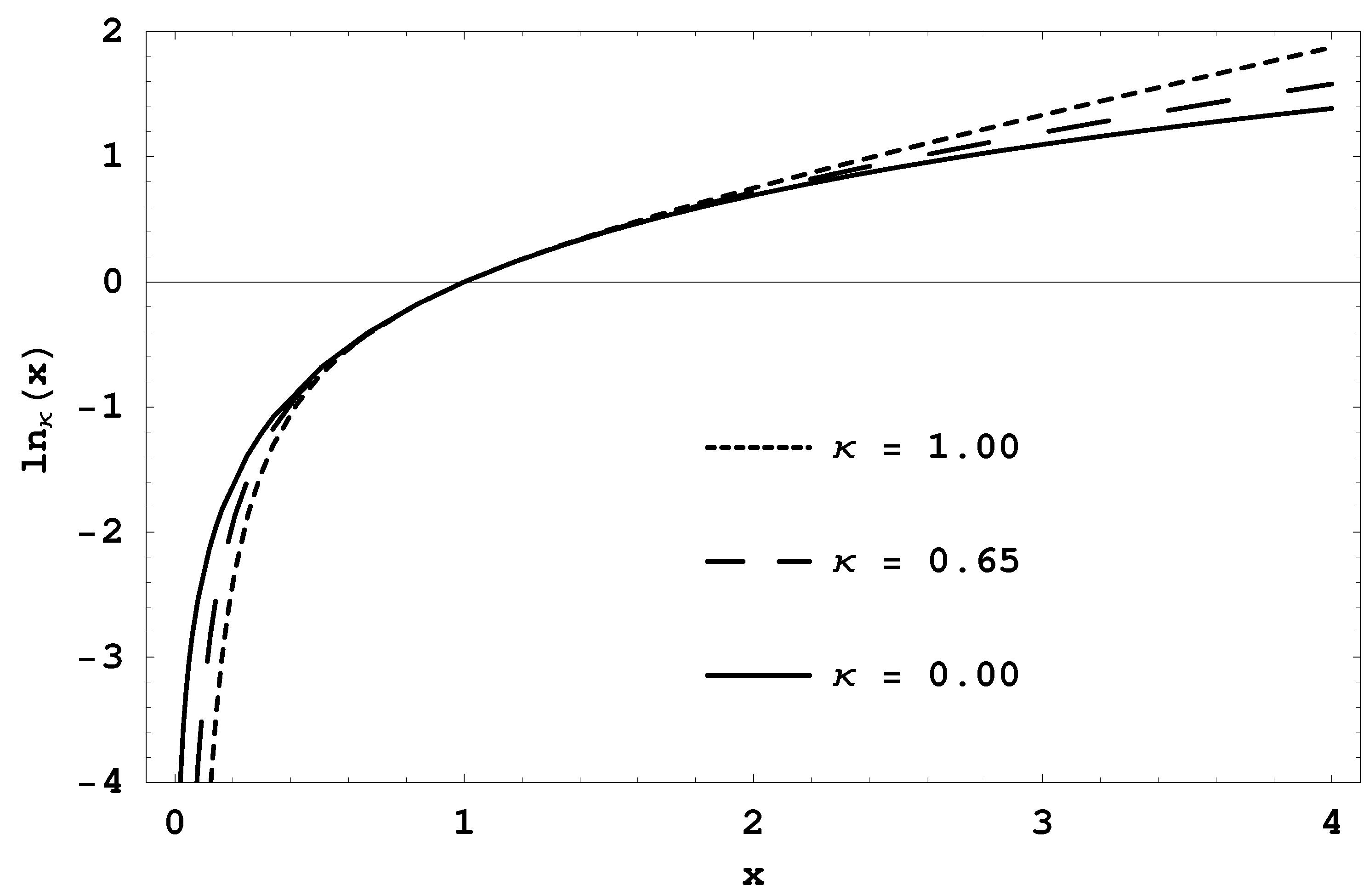
The Taylor expansion of ${exp}_{\kappa }\left(x\right)$ given in [3] can be written also in the following form:

$${exp}_{\kappa }\left(x\right)=\sum _{n=0}^{\infty }\frac{x^n}{n{!}_{\kappa }};{\kappa }^2{x}^2<1$$

(62)

where the symbol, $n{!}_{\kappa }$, representing the κ-generalization of the ordinary factorial, $n!$, recovered for $\kappa =0$, is given by:

$$n{!}_{\kappa }=\frac{n!}{{\xi }_n\left(\kappa \right)}$$

(63)

and the polynomials, ${\xi }_n\left(\kappa \right)$, are defined as:

$$\begin{array}{ccc}& & {\xi }_0\left(\kappa \right)={\xi }_1\left(\kappa \right)=1\hfill \end{array}$$

(64)

$$\begin{array}{ccc}& & {\xi }_n\left(\kappa \right)=\prod _{j=1}^{n-1}\left[1-(2j-n)\kappa \right];n>1\hfill \end{array}$$

(65)

The polynomials, ${\xi }_n\left(\kappa \right)$, for $n>1$, when n is odd, are of the degree $n-1$, with respect to the variable, κ, while when n is even, the degree of ${\xi }_n\left(\kappa \right)$ is $n-2$. The degree of ${\xi }_n\left(\kappa \right)$ is always an even number, and it results:

$$\begin{array}{ccc}& & {\xi }_{2m}\left(\kappa \right)=\prod _{j=0}^{m-1}\left[1-{\left(2j\right)}^2{\kappa }^2\right];m>0\hfill \end{array}$$

(66)

$$\begin{array}{ccc}& & {\xi }_{2m+1}\left(\kappa \right)=\prod _{j=0}^{m-1}\left[1-{(2j+1)}^2{\kappa }^2\right];m>0\hfill \end{array}$$

(67)

The polynomials, ${\xi }_n\left(\kappa \right)$, can be generated by the following simple recursive formula:

$$\begin{array}{ccc}& & {\xi }_0\left(\kappa \right)={\xi }_1\left(\kappa \right)=1\hfill \end{array}$$

(68)

$$\begin{array}{ccc}& & {\xi }_{n+2}\left(\kappa \right)=(1-n^2{\kappa }^2){\xi }_n\left(\kappa \right);n\ge 0\hfill \end{array}$$

(69)

The first nine polynomials read as:

$$\begin{array}{ccc}& & {\xi }_0\left(\kappa \right)={\xi }_1\left(\kappa \right)={\xi }_2\left(\kappa \right)=1\hfill \end{array}$$

(70)

$$\begin{array}{ccc}& & {\xi }_3\left(\kappa \right)=1-{\kappa }^2\hfill \end{array}$$

(71)

$$\begin{array}{ccc}& & {\xi }_4\left(\kappa \right)=1-4{\kappa }^2\hfill \end{array}$$

(72)

$$\begin{array}{ccc}& & {\xi }_5\left(\kappa \right)=(1-{\kappa }^2)(1-9{\kappa }^2)\hfill \end{array}$$

(73)

$$\begin{array}{ccc}& & {\xi }_6\left(\kappa \right)=(1-4{\kappa }^2)(1-16{\kappa }^2)\hfill \end{array}$$

(74)

$$\begin{array}{ccc}& & {\xi }_7\left(\kappa \right)=(1-{\kappa }^2)(1-9{\kappa }^2)(1-25{\kappa }^2)\hfill \end{array}$$

(75)

$$\begin{array}{ccc}& & {\xi }_8\left(\kappa \right)=(1-4{\kappa }^2)(1-16{\kappa }^2)(1-36{\kappa }^2)\hfill \end{array}$$

(76)

After noting that for a given value of κ, the maximum natural number, N, satisfying the condition $N<2+1/\left|\kappa \right|$ is defined univocally, we can verify easily that for $n=0,1,2,...,N$, it results ${\xi }_n\left(\kappa \right)>0$ and, then, $n{!}_{\kappa }>0$. For $n>N$, the sign of ${\xi }_n\left(\kappa \right)$ and, then, of $n{!}_{\kappa }$ alternates with periodicity $--++--++...$

From Equation (63) and (69) follows the recursive formula:

$$(n+2){!}_{\kappa }=\frac{(n+1)(n+2)}{1-n^2{\kappa }^2}n{!}_{\kappa }$$

(77)

By direct comparison of Equation (61) and Equation (77), we obtain the relationship:

$$\begin{array}{c}\hfill n{!}_{\kappa }=\left(1-{\kappa }^2{n}^2\right)n{\int }_0^{\infty }{t}^{n-1}{exp}_{\kappa }(-t)dt\end{array}$$

(78)

It is remarkable that the first three terms in the Taylor expansion of ${exp}_{\kappa }\left(x\right)$ are the same as the ordinary exponential:

$${exp}_{\kappa }\left(x\right)=1+x+\frac{x^2}{2}+(1-{\kappa }^2)\frac{x^3}{3!}+...$$

(79)

4.5. The Function ${\Gamma }_{\kappa }\left(x\right)$

The ${\Gamma }_{\kappa }\left(n\right)$ with an n integer is defined through:

$$\begin{array}{c}\hfill {\Gamma }_{\kappa }\left(n\right)=(n-1){!}_{\kappa }\end{array}$$

(80)

and represents a generalization of the Euler $\Gamma \left(n\right)$ function. In particular, we have ${\Gamma }_{\kappa }\left(1\right)={\Gamma }_{\kappa }\left(2\right)=1$ and ${\Gamma }_{\kappa }\left(3\right)=2$. This definition and the relationship in Equation (78) suggests the following one parameter generalization of the Euler $\Gamma \left(x\right)$ function, i.e., ${\Gamma }_{\kappa }\left(x\right)$, given by:

$$\begin{array}{c}\hfill {\Gamma }_{\kappa }\left(x\right)=\left[1-{\kappa }^2{(x-1)}^2\right](x-1){\int }_0^{\infty }{t}^{x-2}{exp}_{\kappa }(-t)dt\end{array}$$

(81)

The explicit expression of ${\Gamma }_{\kappa }\left(x\right)$ in terms of the ordinary $\Gamma \left(x\right)$ is given by:

$$\begin{array}{c}\hfill {\Gamma }_{\kappa }\left(x\right)=\frac{1-\left|\kappa \right|(x-1)}{{\left|2\kappa \right|}^{x-1}}\frac{\Gamma \left(\frac{1}{\left|2\kappa \right|}-\frac{x-1}{2}\right)}{\Gamma \left(\frac{1}{\left|2\kappa \right|}+\frac{x-1}{2}\right)}\Gamma \left(x\right)\end{array}$$

(82)

and can be used as the definition of ${\Gamma }_{\kappa }\left(x\right)$ when x is a complex variable. Clearly, in the $\kappa \to 0$ limit, it results ${\Gamma }_0\left(x\right)=\Gamma \left(x\right)$. An expression of ${\Gamma }_{\kappa }\left(x\right)$ in terms of the Beta function is the following:

$$\begin{array}{c}\hfill {\Gamma }_{\kappa }\left(x\right)=\frac{1-\left|\kappa \right|(x-1)}{{\left|2\kappa \right|}^{x-1}}(x-1)B\left(\frac{1}{\left|2\kappa \right|}-\frac{x-1}{2},x-1\right)\end{array}$$

(83)

From Equation (61) and Equation (81) follows the property:

$$\begin{array}{c}\hfill {\Gamma }_{\kappa }(x+2)=\frac{x(x+1)}{1-{\kappa }^2{(x-1)}^2}{\Gamma }_{\kappa }\left(x\right)\end{array}$$

(84)

The Taylor expansion of ${exp}_{\kappa }\left(x\right)$ can be written also in the form:

$${exp}_{\kappa }\left(x\right)=\sum _{n=0}^{\infty }\frac{x^n}{{\Gamma }_{\kappa }(n+1)};{\kappa }^2{x}^2<1$$

(85)

In Figure 2 and Figure 3 is plotted the function, ${\Gamma }_{\kappa }\left(x\right)$, defined in Equation (82) in the ranges $-4<x<4$ and $9<x<12$, respectively, for $\kappa =0$ and $\kappa =0.15$. The continuous curve corresponding to $\kappa =0$ is the ordinary Gamma function, $\Gamma \left(x\right)$.

Figure 2. Plot of the function, ${\Gamma }_{\kappa }\left(x\right)$, defined in Equation (82) in the range $-4<x<4$ for $\kappa =0$ and $\kappa =0.15$. The continuous curve corresponding to $\kappa =0$ is the ordinary Gamma function, $\Gamma \left(x\right)$.

Figure 2. Plot of the function, ${\Gamma }_{\kappa }\left(x\right)$, defined in Equation (82) in the range $-4<x<4$ for $\kappa =0$ and $\kappa =0.15$. The continuous curve corresponding to $\kappa =0$ is the ordinary Gamma function, $\Gamma \left(x\right)$.

The incomplete ${\gamma }_{\kappa }(r,x)$ and ${\Gamma }_{\kappa }(r,x)$ are defined as:

$$\begin{array}{c}\hfill {\gamma }_{\kappa }(r,x)=\left[1-{\kappa }^2{(r-1)}^2\right](r-1){\int }_0^x{t}^{r-2}{exp}_{\kappa }(-t)dt\end{array}$$

(86)

$$\begin{array}{c}\hfill {\Gamma }_{\kappa }(r,x)=\left[1-{\kappa }^2{(r-1)}^2\right](r-1){\int }_x^{\infty }{t}^{r-2}{exp}_{\kappa }(-t)dt\end{array}$$

(87)

and hold the following relationships:

$$\begin{array}{ccc}& & {\gamma }_{\kappa }(r,x)+{\Gamma }_{\kappa }(r,x)={\Gamma }_{\kappa }\left(r\right)\hfill \end{array}$$

(88)

$$\begin{array}{ccc}& & {\gamma }_{\kappa }(r,\infty )={\Gamma }_{\kappa }\left(r\right)\hfill \end{array}$$

(89)

$$\begin{array}{ccc}& & {\gamma }_{\kappa }(r,x)=(r-1)\left[1-{\kappa }^2{(r-1)}^2\right]{\mathcal{M}}_{\kappa }(r-1,x)\hfill \end{array}$$

(90)

Figure 3. Plot of the function, ${\Gamma }_{\kappa }\left(x\right)$, defined in Equation (82) in the range $9<x<12$ for $\kappa =0$ and $\kappa =0.15$. The continuous curve corresponding to $\kappa =0$ is the ordinary Gamma function, $\Gamma \left(x\right)$.

Figure 3. Plot of the function, ${\Gamma }_{\kappa }\left(x\right)$, defined in Equation (82) in the range $9<x<12$ for $\kappa =0$ and $\kappa =0.15$. The continuous curve corresponding to $\kappa =0$ is the ordinary Gamma function, $\Gamma \left(x\right)$.

4.6. Expansion in Ordinary Exponentials

Starting from Expression (32) in Equation ${exp}_{\kappa }\left(x\right)$ and the Taylor expansion of the function, $\mathrm{arcsinh}\left(x\right)$, we obtain:

$$\begin{array}{c}\hfill {exp}_{\kappa }\left(x\right)=exp\left(\sum _{n=0}^{\infty }{c}_n{\kappa }^{2n}{x}^{2n+1}\right),{\kappa }^2{x}^2\le 1\end{array}$$

(91)

with:

$$\begin{array}{c}\hfill c_n=\frac{{(-1)}^n\left(2n\right)!}{(2n+1)2^{2n}{(n!)}^2}\end{array}$$

(92)

Exploiting this relationship, we can write ${exp}_{\kappa }\left(x\right)$ as an infinite product of ordinary exponentials:

$$\begin{array}{c}\hfill {exp}_{\kappa }\left(x\right)=\prod _{n=0}^{\infty }exp\left(c_n{\kappa }^{2n}{x}^{2n+1}\right)\end{array}$$

(93)

On the other hand, ${exp}_{\kappa }\left(x\right)$ can be viewed as a continuous linear combination of an infinity of standard exponentials. Namely, for $\mathrm{Re}s\ge 0$, the following Laplace transform holds:

$${exp}_{\kappa }(-s)={\int }_0^{\infty }\frac{1}{\kappa x}{J}_{{}_{1/\kappa }}\left(\frac{x}{\kappa }\right)exp(-sx)dx$$

(94)

$J_{\nu }\left(x\right)$ being the Bessel function.

4.7. The κ-Laplace Transform

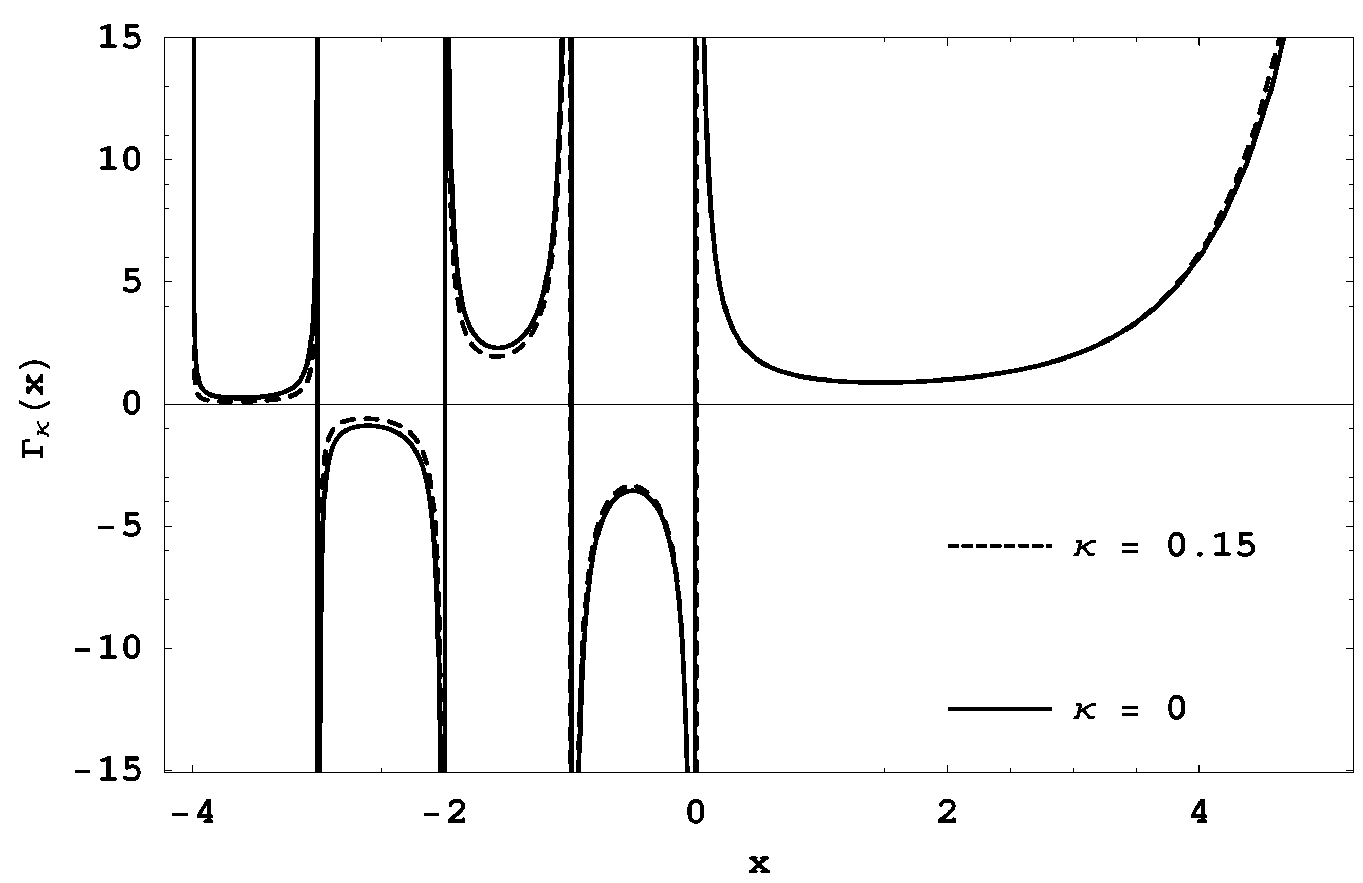
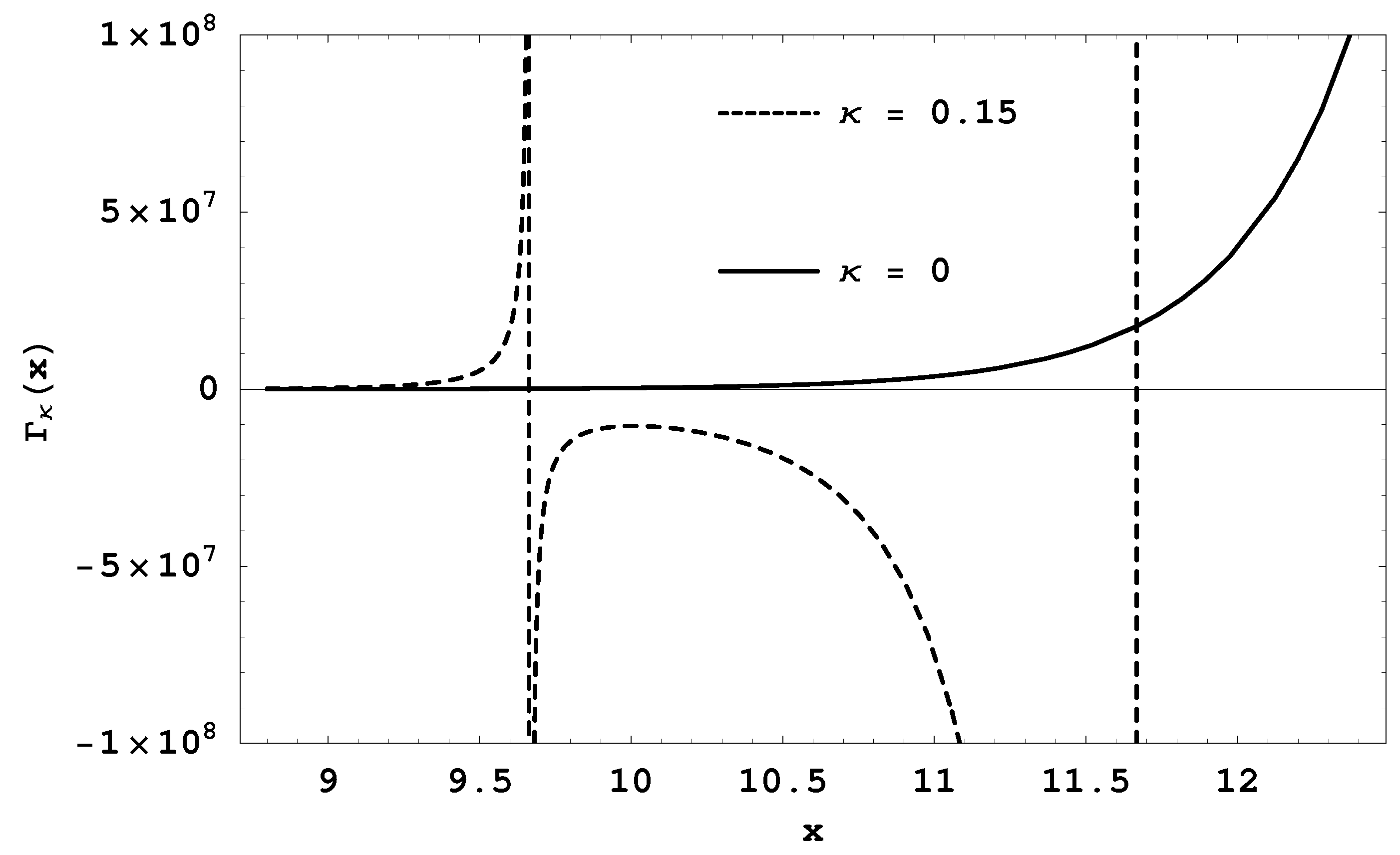
The following κ-Laplace transform emerges naturally:

$$\begin{array}{c}\hfill F_{\kappa }\left(s\right)={\mathcal{L}}_{\kappa }\left\{f\left(t\right)\right\}\left(s\right)={\int }_0^{\infty }f\left(t\right){\left[{exp}_{\kappa }(-t)\right]}^{s}dt\end{array}$$

(95)

as a generalization of the ordinary Laplace transform. The inverse κ-Laplace transform is given by:

$$\begin{array}{c}\hfill f\left(t\right)={\mathcal{L}}_{\kappa }^{-1}\left\{F_{\kappa }\left(s\right)\right\}\left(t\right)=\frac{1}{2\pi i}{\int }_{c-i\infty }^{c+i\infty }{F}_{\kappa }\left(s\right)\frac{{\left[{exp}_{\kappa }\left(t\right)\right]}^s}{\sqrt{1+{\kappa }^2{t}^2}}ds\end{array}$$

(96)

In [34], the mathematical properties of the κ-Laplace transform have been investigated systematically. In Table 1 are reported the main properties of the κ-Laplace transform, which in the $\kappa \to 0$ limit reduce to the corresponding ordinary Laplace transform properties.

Table 1. Properties of the κ-Laplace transform.

$f\left(t\right)$	$F_{\kappa }\left(s\right)$
$af\left(t\right)+bg\left(t\right)$	$a{F}_{\kappa }\left(s\right)+b{G}_{\kappa }\left(s\right)$
$f\left(at\right)$	$\frac{1}{a}{F}_{\kappa /a}\left(\frac{s}{a}\right)$
$f\left(t\right){\left[{exp}_{\kappa }(-t)\right]}^a$	$F_{\kappa }(s-a)$
$\frac{df\left(t\right)}{dt}$	$s{\mathcal{L}}_{\kappa }\left\{\frac{f\left(t\right)}{\sqrt{1+{\kappa }^2{t}^2}}\right\}\left(s\right)-f\left(0\right)$
$\frac{d}{dt}\sqrt{1+{\kappa }^2{t}^2}f\left(t\right)$	$s{F}_{\kappa }\left(s\right)-f\left(0\right)$
$\frac{1}{\sqrt{1+{\kappa }^2{t}^2}}{\int }_0^{t}f\left(w\right)dw$	$\frac{1}{s}{F}_{\kappa }\left(s\right)$
$f\left(t\right){[ln\left({exp}_{\kappa }\left(t\right)\right)]}^n$	${(-1)}^n\frac{d^n{F}_{\kappa }\left(s\right)}{d{s}^n}$
$f\left(t\right){[ln\left({exp}_{\kappa }\left(t\right)\right)]}^{-n}$	${\int }_s^{+\infty }d{w}_n{\int }_{w_n}^{+\infty }d{w}_{n-1}...{\int }_{w_3}^{+\infty }d{w}_2{\int }_{w_2}^{+\infty }d{w}_1{F}_{\kappa }\left(w_1\right)$

Table 1. Properties of the κ-Laplace transform.

$f\left(t\right)$	$F_{\kappa }\left(s\right)$
$af\left(t\right)+bg\left(t\right)$	$a{F}_{\kappa }\left(s\right)+b{G}_{\kappa }\left(s\right)$
$f\left(at\right)$	$\frac{1}{a}{F}_{\kappa /a}\left(\frac{s}{a}\right)$
$f\left(t\right){\left[{exp}_{\kappa }(-t)\right]}^a$	$F_{\kappa }(s-a)$
$\frac{df\left(t\right)}{dt}$	$s{\mathcal{L}}_{\kappa }\left\{\frac{f\left(t\right)}{\sqrt{1+{\kappa }^2{t}^2}}\right\}\left(s\right)-f\left(0\right)$
$\frac{d}{dt}\sqrt{1+{\kappa }^2{t}^2}f\left(t\right)$	$s{F}_{\kappa }\left(s\right)-f\left(0\right)$
$\frac{1}{\sqrt{1+{\kappa }^2{t}^2}}{\int }_0^{t}f\left(w\right)dw$	$\frac{1}{s}{F}_{\kappa }\left(s\right)$
$f\left(t\right){[ln\left({exp}_{\kappa }\left(t\right)\right)]}^n$	${(-1)}^n\frac{d^n{F}_{\kappa }\left(s\right)}{d{s}^n}$
$f\left(t\right){[ln\left({exp}_{\kappa }\left(t\right)\right)]}^{-n}$	${\int }_s^{+\infty }d{w}_n{\int }_{w_n}^{+\infty }d{w}_{n-1}...{\int }_{w_3}^{+\infty }d{w}_2{\int }_{w_2}^{+\infty }d{w}_1{F}_{\kappa }\left(w_1\right)$

Furthermore, the initial value theorem holds:

$$\begin{array}{c}\hfill \underset{t\to 0}{lim}f\left(t\right)=\underset{s\to \infty }{lim}s{F}_{\kappa }\left(s\right)\end{array}$$

(97)

and the final value theorem:

$$\begin{array}{c}\hfill \underset{t\to \infty }{lim}\left|\kappa \right|tf\left(t\right)=\underset{s\to 0}{lim}s{F}_{\kappa }\left(s\right)\end{array}$$

(98)

The κ-convolution of two functions, $f\stackrel{\kappa }{*}g=\left(f\stackrel{\kappa }{*}g\right)\left(t\right)$, is defined as:

$$\begin{array}{c}\hfill f\stackrel{\kappa }{*}g={\int }_0^{t}f\left(t\stackrel{\kappa }{\ominus }\tau \right)g\left(\tau \right)\frac{1-{\kappa }^2\tau (t-\tau )}{\sqrt{1+{\kappa }^2{\tau }^2}}d\tau \end{array}$$

(99)

and has the following properties:

$$\begin{array}{ccc}& & f\stackrel{\kappa }{*}(ag+bh)=a\left(f\stackrel{\kappa }{*}g\right)+b\left(f\stackrel{\kappa }{*}h\right)\hfill \end{array}$$

(100)

$$\begin{array}{ccc}& & f\stackrel{\kappa }{*}g=g\stackrel{\kappa }{*}f\hfill \end{array}$$

(101)

$$\begin{array}{ccc}& & f\stackrel{\kappa }{*}\left(g\stackrel{\kappa }{*}h\right)=\left(f\stackrel{\kappa }{*}g\right)\stackrel{\kappa }{*}h\hfill \end{array}$$

(102)

the following κ-convolution theorem holds:

$$\begin{array}{c}\hfill {\mathcal{L}}_{\kappa }\left\{f\stackrel{\kappa }{*}g\right\}={\mathcal{L}}_{\kappa }\left\{f\right\}{\mathcal{L}}_{\kappa }\left\{g\right\}\end{array}$$

(103)

In Table 2 are reported the κ-Laplace transforms for the delta function, for the unit function and for the power function. We note that the κ-Laplace transform of the power function $f\left(t\right)=t^{\nu -1}$ involves the κ-generalized Gamma function. All the κ-Laplace transforms in the $\kappa \to 0$ limit reduce to the corresponding ordinary Laplace transforms.

Table 2. The κ-Laplace transform of the Dirac delta-function, of the Heaviside unit function and of the power function.

$f\left(t\right)$	$F_{\kappa }\left(s\right)$
$\delta (t-\tau )$	${\left[{exp}_{\kappa }(-\tau )\right]}^s$
$u(t-\tau )$	$\frac{s\sqrt{1+{\kappa }^2{\tau }^2}+{\kappa }^2\tau }{s^2-{\kappa }^2}{\left[{exp}_{\kappa }(-\tau )\right]}^s$
$t^{\nu -1}$	$\frac{s^2}{s^2-{\kappa }^2{\nu }^2}\frac{{\Gamma }_{\frac{\kappa }{s}}(\nu +1)}{\nu s^{\nu }}=\frac{s}{s+\left|\kappa \right|\nu }\frac{\Gamma \left(\nu \right)}{{\left|2\kappa \right|}^{\nu }}\frac{\Gamma \left(\frac{s}{\left|2\kappa \right|}-\frac{\nu }{2}\right)}{\Gamma \left(\frac{s}{\left|2\kappa \right|}+\frac{\nu }{2}\right)}$
$t^{2m-1},m\in Z^{+}$	$\frac{(2m-1)!}{{\prod }_{j=1}^m\left[s^2-{\left(2j\right)}^2{\kappa }^2\right]}$
$t^{2m},m\in Z^{+}$	$\frac{\left(2m\right)!s}{{\prod }_{j=1}^{m+1}\left[s^2-{(2j-1)}^2{\kappa }^2\right]}$

Table 2. The κ-Laplace transform of the Dirac delta-function, of the Heaviside unit function and of the power function.

$f\left(t\right)$	$F_{\kappa }\left(s\right)$
$\delta (t-\tau )$	${\left[{exp}_{\kappa }(-\tau )\right]}^s$
$u(t-\tau )$	$\frac{s\sqrt{1+{\kappa }^2{\tau }^2}+{\kappa }^2\tau }{s^2-{\kappa }^2}{\left[{exp}_{\kappa }(-\tau )\right]}^s$
$t^{\nu -1}$	$\frac{s^2}{s^2-{\kappa }^2{\nu }^2}\frac{{\Gamma }_{\frac{\kappa }{s}}(\nu +1)}{\nu s^{\nu }}=\frac{s}{s+\left|\kappa \right|\nu }\frac{\Gamma \left(\nu \right)}{{\left|2\kappa \right|}^{\nu }}\frac{\Gamma \left(\frac{s}{\left|2\kappa \right|}-\frac{\nu }{2}\right)}{\Gamma \left(\frac{s}{\left|2\kappa \right|}+\frac{\nu }{2}\right)}$
$t^{2m-1},m\in Z^{+}$	$\frac{(2m-1)!}{{\prod }_{j=1}^m\left[s^2-{\left(2j\right)}^2{\kappa }^2\right]}$
$t^{2m},m\in Z^{+}$	$\frac{\left(2m\right)!s}{{\prod }_{j=1}^{m+1}\left[s^2-{(2j-1)}^2{\kappa }^2\right]}$

5. The Function ${ln}_{\kappa }\left(x\right)$

5.1. Definition and Basic Properties

The function, ${ln}_{\kappa }\left(x\right)$, is defined as the inverse function of ${exp}_{\kappa }\left(x\right)$, namely:

$$\begin{array}{c}\hfill {ln}_{\kappa }\left({exp}_{\kappa }x\right)={exp}_{\kappa }\left({ln}_{\kappa }x\right)=x\end{array}$$

(104)

and is given by:

$$\begin{array}{c}\hfill {ln}_{\kappa }\left(x\right)=[lnx]\end{array}$$

(105)

and then:

$$\begin{array}{c}\hfill {ln}_{\kappa }\left(x\right)=\frac{1}{\kappa }sinh(\kappa lnx)\end{array}$$

(106)

or more properly:

$$\begin{array}{c}\hfill {ln}_{\kappa }\left(x\right)=\frac{x^{\kappa }-x^{-\kappa }}{2\kappa }\end{array}$$

(107)

It results that:

$$\begin{array}{ccc}& & {ln}_0\left(x\right)\equiv \underset{\kappa \to 0}{lim}{ln}_{\kappa }\left(x\right)=ln\left(x\right)\hfill \end{array}$$

(108)

$$\begin{array}{ccc}& & {ln}_{-\kappa }\left(x\right)={ln}_{\kappa }\left(x\right)\hfill \end{array}$$

(109)

The function, ${ln}_{\kappa }\left(x\right)$, just as the ordinary logarithm, has the properties:

$$\begin{array}{ccc}& & {ln}_{\kappa }\left(x\right)\in C^{\infty }\left({\mathbf{R}}^{+}\right)\hfill \end{array}$$

(110)

$$\begin{array}{ccc}& & \frac{d}{dx}{ln}_{\kappa }\left(x\right)>0\hfill \end{array}$$

(111)

$$\begin{array}{ccc}& & {ln}_{\kappa }\left(0^{+}\right)=-\infty \hfill \end{array}$$

(112)

$$\begin{array}{ccc}& & {ln}_{\kappa }\left(1\right)=0\hfill \end{array}$$

(113)

$$\begin{array}{ccc}& & {ln}_{\kappa }(+\infty )=+\infty \hfill \end{array}$$

(114)

$$\begin{array}{ccc}& & {ln}_{\kappa }(1/x)=-{ln}_{\kappa }\left(x\right)\hfill \end{array}$$

(115)

In Figure 4 is plotted the function, ${ln}_{\kappa }\left(x\right)$, defined in Equation (107) for three different values of the parameter of κ. The continuous curve corresponding to $\kappa =0$ is the ordinary logarithm function, $ln\left(x\right)$.

Figure 4. Plot of the function, ${ln}_{\kappa }\left(x\right)$, defined by Equation (107) for three different values of the parameter of κ. The continuous curve corresponding to $\kappa =0$ is the ordinary logarithm function, $ln\left(x\right)$.

Figure 4. Plot of the function, ${ln}_{\kappa }\left(x\right)$, defined by Equation (107) for three different values of the parameter of κ. The continuous curve corresponding to $\kappa =0$ is the ordinary logarithm function, $ln\left(x\right)$.

Furthermore, ${ln}_{\kappa }\left(x\right)$ has the two properties:

$$\begin{array}{ccc}& & {ln}_{\kappa }\left(x^r\right)=r{ln}_{r\kappa }\left(x\right)\hfill \end{array}$$

(116)

$$\begin{array}{ccc}& & {ln}_{\kappa }\left(xy\right)={ln}_{\kappa }\left(x\right)\oplus {}^{{}^{\kappa }}{ln}_{\kappa }\left(y\right)\hfill \end{array}$$

(117)

with $r\in \mathbf{R}$. Note that property in Equation (115) follows as a particular case of property in Equation (117).

We remark the following concavity properties:

$$\begin{array}{ccc}& & \frac{d^2}{d{x}^2}{ln}_{\kappa }\left(x\right)<0\hfill \end{array}$$

(118)

$$\begin{array}{ccc}& & \frac{d^2}{d{x}^2}x{ln}_{\kappa }\left(x\right)<0\hfill \end{array}$$

(119)

A very interesting property of this function is its power law asymptotic behavior:

$$\begin{array}{ccc}& & {ln}_{\kappa }\left(x\right)\genfrac{}{}{0pt}{}{}{\stackrel{\sim }{x\to 0^{+}}}-\frac{1}{2\left|\kappa \right|}{x}^{-\left|\kappa \right|}\hfill \end{array}$$

(120)

$$\begin{array}{ccc}& & {ln}_{\kappa }\left(x\right)\genfrac{}{}{0pt}{}{}{\stackrel{\sim }{x\to +\infty }}\frac{1}{2\left|\kappa \right|}{x}^{\left|\kappa \right|}\hfill \end{array}$$

(121)

After recalling the integral representation of the ordinary logarithm:

$$ln\left(x\right)=\frac{1}{2}{\int }_{1/x}^x\frac{1}{t}dt$$

(122)

one can verify that the latter relationship can be generalized easily in order to obtain ${ln}_{\kappa }\left(x\right)$, by replacing the integrand function $y_0\left(t\right)=t^{-1}$ by the new function $y_{\kappa }\left(t\right)=t^{-1-\kappa }$, namely:

$${ln}_{\kappa }\left(x\right)=\frac{1}{2}{\int }_{1/x}^x\frac{1}{t^{1+\kappa }}dt$$

(123)

5.2. Taylor Expansion

The Taylor expansion of ${ln}_{\kappa }(1+x)$ converges if $-1<x\le 1$ and assumes the form:

$${ln}_{\kappa }(1+x)=\sum _{n=1}^{\infty }{b}_n\left(\kappa \right){(-1)}^{n-1}\frac{x^n}{n}$$

(124)

with $b_1\left(\kappa \right)=1$, while for $n>1$, $b_n\left(\kappa \right)$ is given by:

$$\begin{array}{ccc}\hfill b_n\left(\kappa \right)& & =\frac{1}{2}\left(1-\kappa \right)\left(1-\frac{\kappa }{2}\right)...\left(1-\frac{\kappa }{n-1}\right)\hfill \end{array}$$

$$\begin{array}{ccc}& & +\frac{1}{2}\left(1+\kappa \right)\left(1+\frac{\kappa }{2}\right)...\left(1+\frac{\kappa }{n-1}\right)\hfill \end{array}$$

(125)

It results $b_n\left(0\right)=1$ and $b_n(-\kappa )=b_n\left(\kappa \right)$. The first terms of the expansion are:

$${ln}_{\kappa }(1+x)=x-\frac{x^2}{2}+\left(1+\frac{{\kappa }^2}{2}\right)\frac{x^3}{3}-...$$

(126)

5.3. The Function ${\Gamma }_{\kappa }\left(x\right)$

The following integral is useful:

$$\begin{array}{ccc}& & {\int }_0^1{\left({ln}_{\kappa }\frac{1}{x}\right)}^{r-1}dx\hfill \end{array}$$

$$\begin{array}{ccc}& & =\frac{{\left|2\kappa \right|}^{1-r}}{1+(r-1)\left|\kappa \right|}\frac{\Gamma \left(\frac{1}{\left|2\kappa \right|}-\frac{r-1}{2}\right)}{\Gamma \left(\frac{1}{\left|2\kappa \right|}+\frac{r-1}{2}\right)}\Gamma \left(r\right)\hfill \end{array}$$

(127)

Starting from the definition of the generalized Euler gamma function, i.e., ${\Gamma }_{\kappa }\left(x\right)$ given in the previous section, we can write it also in the following alternative, but equivalent form:

$$\begin{array}{c}\hfill {\Gamma }_{\kappa }\left(x\right)=\left[1-{\kappa }^2{(x-1)}^2\right]{\int }_0^1{\left({ln}_{\kappa }\frac{1}{t}\right)}^{x-1}dt\end{array}$$

(128)

An expression of ${\Gamma }_{\kappa }\left(x\right)$, where the parameter κ enters exclusively through the function, ${ln}_{\kappa }(.)$, follows easily:

$$\begin{array}{c}\hfill {\Gamma }_{\kappa }\left(x\right)=(x-1)\frac{{\int }_0^1{\left({ln}_{\kappa }\frac{1}{t}\right)}^{x-1}dt}{{\int }_0^1{ln}_{\kappa }{\left(\frac{1}{t}\right)}^{x-1}dt}\end{array}$$

(129)

From the latter relationships, it follows that $n{!}_{\kappa }$ is given by:

$$\begin{array}{c}\hfill n{!}_{\kappa }=\left(1-{\kappa }^2{n}^2\right){\int }_0^1{\left({ln}_{\kappa }\frac{1}{t}\right)}^{n}dt=n\frac{{\int }_0^1{\left({ln}_{\kappa }\frac{1}{t}\right)}^{n}dt}{{\int }_0^1{ln}_{\kappa }{\left(\frac{1}{t}\right)}^{n}dt}\end{array}$$

(130)

5.4. ${ln}_{\kappa }\left(x\right)$ as the Solution of a Functional Equation

The logarithm $y\left(x\right)=ln\left(x\right)$ is the only existing function, unless a multiplicative constant, which results in being the solution of the function equation $y\left(x_1{x}_2\right)=y\left(x_1\right)+y\left(x_2\right)$. Let us consider now the generalization of this equation, obtained by substituting the ordinary sum by the generalized sum:

$$\begin{array}{c}\hfill y\left(x_1{x}_2\right)=y\left(x_1\right)\stackrel{\kappa }{\oplus }y\left(x_2\right)\end{array}$$

(131)

We proceed by solving this equation, which assumes the explicit form:

$$\begin{array}{ccc}\hfill y\left(x_1{x}_2\right)& =& y\left(x_1\right)\sqrt{1+{\kappa }^{2}y\left(x_2\right){}^2}\hfill \end{array}$$

$$\begin{array}{ccc}& +& y\left(x_2\right)\sqrt{1+{\kappa }^{2}y\left(x_1\right){}^2}\hfill \end{array}$$

(132)

After performing the substitution $y\left(x\right)={\kappa }^{-1}sinh\kappa g\left(x\right)$, we obtain that the auxiliary function, $g\left(x\right)$, obeys the equation $g\left(x_1{x}_2\right)=g\left(x_1\right)+g\left(x_2\right)$ and, then, is given by $g\left(x\right)=Alnx$. The unknown function, $y\left(x\right)$, becomes $y\left(x\right)={\kappa }^{-1}sinh(\kappa lnx)$ where we have set $A=1$ in order to recover, in the limit $\kappa \to 0$, the classical solution $y\left(x\right)=ln\left(x\right)$. Then, we can conclude that the solution of Equation (uid135) is given by:

$$\begin{array}{c}\hfill y\left(x\right)={ln}_{\kappa }\left(x\right)\end{array}$$

(133)

5.5. ${ln}_{\kappa }\left(x\right)$ as the Solution of a Differential-Functional Equation

The following first order differential-functional equation emerges in statistical mechanics within the context of the maximum entropy principle:

$$\begin{array}{ccc}& & \frac{d}{dx}\left[xf\left(x\right)\right]=\frac{1}{\gamma }f\left(ϵx\right)\hfill \end{array}$$

(134)

$$\begin{array}{ccc}& & f\left(1\right)=0\hfill \end{array}$$

(135)

$$\begin{array}{ccc}& & f^{\prime }\left(1\right)=1\hfill \end{array}$$

(136)

$$\begin{array}{ccc}& & f\left(1/x\right)=-f\left(x\right)\hfill \end{array}$$

(137)

The latter problem admits two solutions [3,9]. The first is given by $f\left(x\right)=ln\left(x\right)$ and $\gamma =1$, $ϵ=e$. The second solution is given by:

$$\begin{array}{c}\hfill f\left(x\right)={ln}_{\kappa }\left(x\right)\end{array}$$

(138)

and:

$$\begin{array}{ccc}& & \gamma =\frac{1}{\sqrt{1-{\kappa }^2}}\hfill \end{array}$$

(139)

$$\begin{array}{ccc}& & ϵ={\left(\frac{1+\kappa }{1-\kappa }\right)}^{1/2\kappa }\hfill \end{array}$$

(140)

The constant, γ, is the Lorentz factor corresponding to the reference velocity $v_{*}$, while the constant, $ϵ={exp}_{\kappa }\left(\gamma \right)$, represents the κ-generalization of the Napier number, e.

5.6. The Entropy

A physically meaningful link between the functions, ${ln}_{\kappa }\left(x\right)$ and ${exp}_{\kappa }\left(x\right)$, is given by a variational principle. The following theorem holds:

Theorem 6. Let $g\left(x\right)$ be an arbitrary real function and $y\left(x\right)$, a probability distribution function of the variable, $x\in A$. The solution of the variational equation:

$$\begin{array}{c}\hfill \frac{\delta }{\delta y\left(x\right)}\left[-{\int }_{A}dxy\left(x\right){ln}_{\kappa }y\left(x\right)+{\int }_{A}dxy\left(x\right)g\left(x\right)\right]=0\end{array}$$

(141)

is unique and is given by:

$$\begin{array}{c}\hfill y\left(x\right)=\frac{1}{ϵ}{exp}_{\kappa }\left(\gamma g\left(x\right)\right)\end{array}$$

(142)

the constants γ and ϵ being defined by Equations (139) and (140), respectively.

The proof of the theorem is trivial and employs Equation (134). This theorem permits us to interpret the functional:

$$\begin{array}{c}\hfill S_{\kappa }=-{\int }_{A}dxy\left(x\right){ln}_{\kappa }y\left(x\right)\end{array}$$

(143)

which can be written also in the form:

$$\begin{array}{c}\hfill S_{\kappa }={\int }_{A}dx\frac{y{\left(x\right)}^{1-\kappa }-y{\left(x\right)}^{1+\kappa }}{2\kappa }\end{array}$$

(144)

as the entropy associated with the function, ${exp}_{\kappa }\left(x\right)$. It is remarkable that in the $\kappa \to 0$ limit, as ${ln}_{\kappa }\left(y\right)$ and ${exp}_{\kappa }\left(x\right)$ approach $ln\left(y\right)$ and $exp\left(x\right)$, respectively, the new entropy reduces to the old Boltzmann-Shannon entropy.

It is shown that the entropy $S_{\kappa }$ has the standard properties of Boltzmann-Shannon entropy: it is thermodynamically and Lesche stable and obeys the Khinchin axioms of continuity, maximality, expandability and generalized additivity.

6. κ-Trigonometry

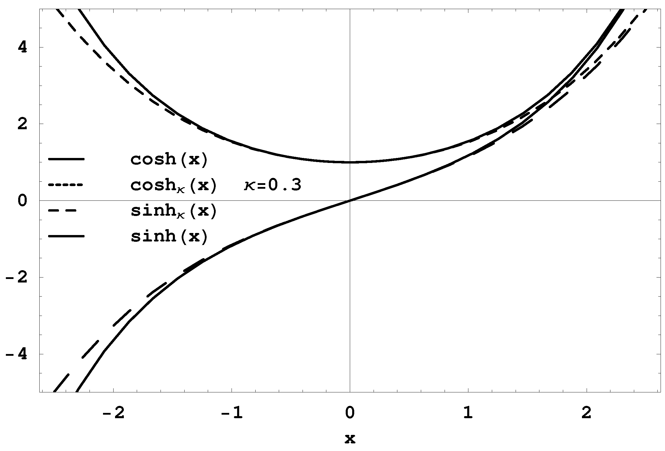
6.1. κ-Hyperbolic Trigonometry

The κ-hyperbolic trigonometry can be introduced by defining the κ-hyperbolic sine and κ-hyperbolic cosine:

$$\begin{array}{c}\hfill {sinh}_{\kappa }\left(x\right)=\frac{{exp}_{\kappa }\left(x\right)-{exp}_{\kappa }(-x)}{2}\end{array}$$

(145)

$$\begin{array}{c}\hfill {cosh}_{\kappa }\left(x\right)=\frac{{exp}_{\kappa }\left(x\right)+{exp}_{\kappa }(-x)}{2}\end{array}$$

(146)

starting from the κ-Euler formula:

$$\begin{array}{c}\hfill {exp}_{\kappa }(\pm x)={cosh}_{\kappa }\left(x\right)\pm {sinh}_{\kappa }\left(x\right)\end{array}$$

(147)

In Figure 5 are plotted the functions, ${sinh}_{\kappa }\left(x\right)$ and ${cosh}_{\kappa }\left(x\right)$, for $\kappa =0.3$ (dashed lines). For comparison, in the same figure are reported the corresponding ordinary functions, $sinh\left(x\right)$ and $cosh\left(x\right)$ (continuous lines).

Figure 5. Plot of the functions, ${sinh}_{\kappa }\left(x\right)$ and ${cosh}_{\kappa }\left(x\right)$, for $\kappa =0.3$ (dashed lines) defined through Equations (145) and (146), respectively. For comparison, in the same plot are reported the corresponding ordinary functions, $sinh\left(x\right)$ and $cosh\left(x\right)$ (continuous lines).

Figure 5. Plot of the functions, ${sinh}_{\kappa }\left(x\right)$ and ${cosh}_{\kappa }\left(x\right)$, for $\kappa =0.3$ (dashed lines) defined through Equations (145) and (146), respectively. For comparison, in the same plot are reported the corresponding ordinary functions, $sinh\left(x\right)$ and $cosh\left(x\right)$ (continuous lines).

The κ-hyperbolic tangent and cotangent functions are defined through:

$$\begin{array}{ccc}& & {tanh}_{\kappa }\left(x\right)=\frac{{sinh}_{\kappa }\left(x\right)}{{cosh}_{\kappa }\left(x\right)}\hfill \end{array}$$

(148)

$$\begin{array}{ccc}& & {coth}_{\kappa }\left(x\right)=\frac{{cosh}_{\kappa }\left(x\right)}{{sinh}_{\kappa }\left(x\right)}\hfill \end{array}$$

(149)

Holding the relationships:

$$\begin{array}{ccc}& & {sinh}_{\kappa }\left(x\right)=sinh\left(\left\{x\right\}\right)\hfill \end{array}$$

(150)

$$\begin{array}{ccc}& & {cosh}_{\kappa }\left(x\right)=cosh\left(\left\{x\right\}\right)\hfill \end{array}$$

(151)

$$\begin{array}{ccc}& & {tanh}_{\kappa }\left(x\right)=tanh\left(\left\{x\right\}\right)\hfill \end{array}$$

(152)

$$\begin{array}{ccc}& & {coth}_{\kappa }\left(x\right)=coth\left(\left\{x\right\}\right)\hfill \end{array}$$

(153)

it is straightforward to verify that κ-hyperbolic trigonometry preserves the same structure of the ordinary hyperbolic trigonometry, which recovers as a special case in the limit $\kappa \to 0$. For instance, from the κ-Euler formula and from ${exp}_{\kappa }(-x){exp}_{\kappa }\left(x\right)=1$, the fundamental formula of the κ-hyperbolic trigonometry follows:

$$\begin{array}{c}\hfill {cosh}_{\kappa }^2\left(x\right)-{sinh}_{\kappa }^2\left(x\right)=1\end{array}$$

(154)

All the formulas of the ordinary hyperbolic trigonometry still hold, after proper generalization. Taking into account that $\left\{x\stackrel{\kappa }{\oplus }y\right\}=\left\{x\right\}+\left\{y\right\}$, it is easy to verify that the generalization of a given formula can be obtained starting from the corresponding ordinary formula and, then, by making in the arguments of the hyperbolic trigonometric functions the substitutions $x+y\to x\stackrel{\kappa }{\oplus }y$ and $x-y\to x\stackrel{\kappa }{\ominus }y$. For instance, it results:

$${sinh}_{\kappa }\left(x\stackrel{\kappa }{\oplus }y\right)+{sinh}_{\kappa }\left(x\stackrel{\kappa }{\ominus }y\right)=2{sinh}_{\kappa }\left(x\right){cosh}_{\kappa }\left(y\right)$$

(155)

$${cosh}_{\kappa }\left(x\stackrel{\kappa }{\oplus }y\right)={cosh}_{\kappa }\left(x\right){cosh}_{\kappa }\left(x\right)+{sinh}_{\kappa }\left(x\right){sinh}_{\kappa }\left(y\right)$$

(156)

$$\begin{array}{c}\hfill {tanh}_{\kappa }\left(x\right)+{tanh}_{\kappa }\left(y\right)=\frac{{sinh}_{\kappa }\left(x\stackrel{\kappa }{\oplus }y\right)}{{cosh}_{\kappa }\left(x\right){cosh}_{\kappa }\left(y\right)}\end{array}$$

(157)

and so on.

Obviously, the substitution $nx\to x\stackrel{\kappa }{\oplus }x\stackrel{\kappa }{\oplus }...\stackrel{\kappa }{\oplus }x=\left[n\right]\stackrel{\kappa }{\otimes }x$ is required, so that, for instance, it holds the formula:

$${sinh}_{\kappa }^4\left(x\right)=\frac{1}{8}\left[{cosh}_{\kappa }\left(\left[4\right]\stackrel{\kappa }{\otimes }x\right)-4{cosh}_{\kappa }\left(\left[2\right]\stackrel{\kappa }{\otimes }x\right)+3\right]$$

(158)

and so on.

The κ-De Moivre formula involving hyperbolic trigonometric functions having arguments of the type $rx$, with $r\in \mathbf{R}$, assumes the form:

$${[{cosh}_{\kappa }\left(x\right)\pm {sinh}_{\kappa }\left(x\right)]}^r={cosh}_{\kappa /r}\left(rx\right)\pm {sinh}_{{}_{\{\kappa /r\}}}\left(rx\right)$$

(159)

Furthermore, the formulas involving the derivatives of the hyperbolic trigonometric function still hold, after being properly generalized. For instance, we have:

$$\begin{array}{ccc}& & \frac{d{sinh}_{\kappa }\left(x\right)}{d_{\kappa }x}={cosh}_{\kappa }\left(x\right)\hfill \end{array}$$

(160)

$$\begin{array}{ccc}& & \frac{d{tanh}_{\kappa }\left(x\right)}{d_{\kappa }x}={cosh}_{\kappa }^{-2}\left(x\right)\hfill \end{array}$$

(161)

and so on.

The κ-inverse hyperbolic functions can be introduced starting from the corresponding ordinary functions. It is trivial to verify that κ-inverse hyperbolic functions are related to the κ-logarithm by the usual formulas of the ordinary mathematics. For instance, we have:

$$\begin{array}{ccc}& & {\mathrm{arcsinh}}_{\kappa }\left(x\right)={ln}_{\kappa }\left(\sqrt{1+x^2}+x\right)\hfill \end{array}$$

(162)

$$\begin{array}{ccc}& & {\mathrm{arccosh}}_{\kappa }\left(x\right)={ln}_{\kappa }\left(\sqrt{x^2-1}+x\right)\hfill \end{array}$$

(163)

$$\begin{array}{ccc}& & {\mathrm{arctanh}}_{\kappa }\left(x\right)={ln}_{\kappa }\sqrt{\frac{1+x}{1-x}}\hfill \end{array}$$

(164)

$$\begin{array}{ccc}& & {\mathrm{arccoth}}_{\kappa }\left(x\right)={ln}_{\kappa }\sqrt{\frac{1-x}{1+x}}\hfill \end{array}$$

(165)

and, consequently, hold:

$$\begin{array}{ccc}\hfill {\mathrm{arcsinh}}_{\kappa }\left(x\right)& =& {\mathrm{arccosh}}_{\kappa }\sqrt{1+x^2}\hfill \end{array}$$

(166)

$$\begin{array}{ccc}\hfill {\mathrm{arcsinh}}_{\kappa }\left(x\right)& =& {\mathrm{arctanh}}_{\kappa }\frac{x}{\sqrt{1+x^2}}\hfill \end{array}$$

(167)

$$\begin{array}{ccc}\hfill {\mathrm{arcsinh}}_{\kappa }\left(x\right)& =& {\mathrm{arccoth}}_{\kappa }\frac{\sqrt{1+x^2}}{x}\hfill \end{array}$$

(168)

From Equation (162) follows the relationship:

$$\begin{array}{c}\hfill {exp}_{\kappa }\left({\mathrm{arcsinh}}_{\kappa }x\right)=exp\left(\mathrm{arcsinh}x\right)\end{array}$$

(169)

Furthermore, the relationship:

$$\begin{array}{c}\hfill {\mathrm{arcsinh}}_{\kappa }\left(x\right)=\frac{1}{\kappa }{sinh}_{1/\kappa }\left(\kappa x\right)\end{array}$$

(170)

involving the function, ${\mathrm{arcsinh}}_{\kappa }\left(x\right)$, follows from Equation (162). Analogous formulas involving ${\mathrm{arccosh}}_{\kappa }\left(x\right)$, ${\mathrm{arctanh}}_{\kappa }\left(x\right)$ or ${\mathrm{arccoth}}_{\kappa }\left(x\right)$ do not hold, instead.

6.2. κ-Cyclic Trigonometry

By employing the generalized κ-Euler formula:

$$\begin{array}{c}\hfill {exp}_{\kappa }(\pm ix)={cos}_{\kappa }\left(x\right)\pm i{sin}_{\kappa }\left(x\right)\end{array}$$

(171)

we introduce the κ-cyclic sine and κ-cosine as:

$$\begin{array}{c}\hfill {sin}_{\kappa }\left(x\right)=\frac{{exp}_{\kappa }\left(ix\right)-{exp}_{\kappa }(-ix)}{2i}\end{array}$$

(172)

$$\begin{array}{c}\hfill {cos}_{\kappa }\left(x\right)=\frac{{exp}_{\kappa }\left(ix\right)+{exp}_{\kappa }(-ix)}{2}\end{array}$$

(173)

while the κ-cyclic tangent and κ-cotangent functions are defined through:

$$\begin{array}{ccc}& & {tan}_{\kappa }\left(x\right)=\frac{{sin}_{\kappa }\left(x\right)}{{cos}_{\kappa }\left(x\right)}\hfill \end{array}$$

(174)

$$\begin{array}{ccc}& & {cot}_{\kappa }\left(x\right)=\frac{{cos}_{\kappa }\left(x\right)}{{sin}_{\kappa }\left(x\right)}\hfill \end{array}$$

(175)

After noting that:

$$\begin{array}{c}\hfill {exp}_{\kappa }\left(ix\right)=exp\left(i\left\{x\right\}\right)\end{array}$$

(176)

with:

$$\begin{array}{c}\hfill \left\{x\right\}=\frac{1}{\kappa }arcsin\kappa x\end{array}$$

(177)

it follows that the cyclic functions are defined in the interval, $-1/\kappa \le x\le 1/\kappa$. The function:

$$\begin{array}{c}\hfill \left[x\right]=\frac{1}{\kappa }sin\kappa x\end{array}$$

(178)

is defined as the inverse of $\left\{x\right\}$, i.e, $\left[\right\{x\left\}\right]=\left\{\right[x\left]\right\}=x$. The κ-sum $\stackrel{\kappa }{\oplus }$ and κ-product $\stackrel{\kappa }{\otimes }$ given by:

$$\begin{array}{ccc}& & x\stackrel{\kappa }{\oplus }y=x\sqrt{1-{\kappa }^2{y}^2}+y\sqrt{1-{\kappa }^2{x}^2}\hfill \end{array}$$

(179)

$$\begin{array}{ccc}& & x\stackrel{\kappa }{\otimes }y=\frac{1}{\kappa }sin\left(\frac{1}{\kappa }\arcsin \left(\kappa x\right)\arcsin \left(\kappa y\right)\right)\hfill \end{array}$$

(180)

are isomorphic operations to the ordinary sum and product respectively, i.e.:

$$\begin{array}{ccc}& & \left\{x\stackrel{\kappa }{\oplus }y\right\}=\left\{x\right\}+\left\{y\right\}\hfill \end{array}$$

(181)

$$\begin{array}{ccc}& & \left\{x\stackrel{\kappa }{\otimes }y\right\}=\left\{x\right\}·\left\{y\right\}\hfill \end{array}$$

(182)

Holding the relationships:

$$\begin{array}{ccc}& & {sin}_{\kappa }\left(x\right)=sin\left(\left\{x\right\}\right)\hfill \end{array}$$

(183)

$$\begin{array}{ccc}& & {cos}_{\kappa }\left(x\right)=cos\left(\left\{x\right\}\right)\hfill \end{array}$$

(184)

$$\begin{array}{ccc}& & {tan}_{\kappa }\left(x\right)=tan\left(\left\{x\right\}\right)\hfill \end{array}$$

(185)

$$\begin{array}{ccc}& & {cot}_{\kappa }\left(x\right)=cot\left(\left\{x\right\}\right)\hfill \end{array}$$

(186)

It is straightforward to verify that the generalized cyclic trigonometry preserves the same structure of the ordinary cyclic trigonometry, which recovers as a special case in the limit $\kappa \to 0$. For instance, the following generalized formulas hold:

$$\begin{array}{ccc}& & {cos}_{\kappa }^2\left(x\right)+{sin}_{\kappa }^2\left(x\right)=1\hfill \end{array}$$

(187)

$$\begin{array}{ccc}& & {sin}_{\kappa }\left(x\stackrel{\kappa }{\oplus }y\right)={sin}_{\kappa }\left(x\right){cos}_{\kappa }\left(y\right)+{cos}_{\kappa }\left(x\right){sin}_{\kappa }\left(y\right)\hfill \end{array}$$

(188)

$$\begin{array}{ccc}& & {cos}_{\kappa }^5\left(x\right)=\frac{1}{16}\left[{cos}_{\kappa }\left(\left[5\right]\stackrel{\kappa }{\otimes }x\right)+5{cos}_{\kappa }\left(\left[3\right]\stackrel{\kappa }{\otimes }x\right)+10{cos}_{\kappa }\left(x\right)\right]\hfill \end{array}$$

(189)

and so on.

After introducing the following κ-deformed derivative operator:

$$\begin{array}{c}\hfill \frac{d}{d_{\kappa }x}=\sqrt{1-{\kappa }^2{x}^2}\frac{d}{dx}\end{array}$$

(190)

we can obtain, easily, further formulas on the cyclic κ-trigonometry emerging as generalizations of the corresponding formulas of the ordinary trigonometry. For instance, we have:

$$\begin{array}{ccc}& & \frac{d{cos}_{\kappa }\left(x\right)}{d_{\kappa }x}=-{sin}_{\kappa }\left(x\right)\hfill \end{array}$$

(191)

$$\begin{array}{ccc}& & \frac{d{cot}_{\kappa }\left(x\right)}{d_{\kappa }x}=-{sin}_{\kappa }^{-2}\left(x\right)\hfill \end{array}$$

(192)

and so on.

The κ-inverse cyclic functions can be calculated by inversion of the corresponding direct functions and are given by:

$$\begin{array}{ccc}& & {\arcsin }_{\kappa }\left(x\right)=-i{ln}_{\kappa }\left(\sqrt{1-x^2}+ix\right)\hfill \end{array}$$

(193)

$$\begin{array}{ccc}& & {\arccos }_{\kappa }\left(x\right)=-i{ln}_{\kappa }\left(\sqrt{x^2-1}+x\right)\hfill \end{array}$$

(194)

$$\begin{array}{ccc}& & {\arctan }_{\kappa }\left(x\right)=i{ln}_{\kappa }\sqrt{\frac{1-ix}{1+ix}}\hfill \end{array}$$

(195)

$$\begin{array}{ccc}& & {\mathrm{arccot}}_{\kappa }\left(x\right)=i{ln}_{\kappa }\sqrt{\frac{ix+1}{ix-1}}\hfill \end{array}$$

(196)

Finally, we note that the κ-cyclic and κ-hyperbolic trigonometric functions are linked through the relationships:

$$\begin{array}{ccc}& & {sin}_{\kappa }\left(x\right)=-i{sinh}_{\kappa }\left(ix\right)\hfill \end{array}$$

(197)

$$\begin{array}{ccc}& & {cos}_{\kappa }\left(x\right)={cosh}_{\kappa }\left(ix\right)\hfill \end{array}$$

(198)

$$\begin{array}{ccc}& & {tan}_{\kappa }\left(x\right)=-i{tanh}_{\kappa }\left(ix\right)\hfill \end{array}$$

(199)

$$\begin{array}{ccc}& & {cot}_{\kappa }\left(x\right)=i{coth}_{\kappa }\left(ix\right)\hfill \end{array}$$

(200)

$$\begin{array}{ccc}& & {\arcsin }_{\kappa }\left(x\right)=-i{\mathrm{arcsinh}}_{\kappa }\left(ix\right)\hfill \end{array}$$

(201)

$$\begin{array}{ccc}& & {\arccos }_{\kappa }\left(x\right)=-i{\mathrm{arccosh}}_{\kappa }\left(x\right)\hfill \end{array}$$

(202)

$$\begin{array}{ccc}& & {\arctan }_{\kappa }\left(x\right)=-i{\mathrm{arctanh}}_{\kappa }\left(ix\right)\hfill \end{array}$$

(203)

$$\begin{array}{ccc}& & {\mathrm{arccot}}_{\kappa }\left(x\right)=i{\mathrm{arccoth}}_{\kappa }\left(ix\right)\hfill \end{array}$$

(204)

which, in the $\kappa \to 0$ limit, reduce to the standard formulas involving the ordinary cyclic and hyperbolic functions.

References

1. Kaniadakis, G. Non-linear kinetics underlying generalized statistics. Physica A 2001, 296, 405–425. [Google Scholar] [CrossRef]
2. Kaniadakis, G. H-theorem and generalized entropies within the framework of nonlinear kinetics. Phys. Lett. A 2001, 288, 283–291. [Google Scholar] [CrossRef]
3. Kaniadakis, G. Statistical mechanics in the context of special relativity. Phys. Rev. E 2002, 66, 056125. [Google Scholar] [CrossRef] [PubMed]
4. Kaniadakis, G. Statistical mechanics in the context of special relativity II. Phys. Rev. E 2005, 72, 036108. [Google Scholar] [CrossRef] [PubMed]
5. Kaniadakis, G. Towards a relativistic statistical theory. Physica A 2006, 365, 17–23. [Google Scholar] [CrossRef]
6. Kaniadakis, G. Relativistic entropy and related Boltzmann kinetics. Eur. Phys. J. A 2009, 40, 275–287. [Google Scholar] [CrossRef]
7. Kaniadakis, G. Maximum entropy principle and power-law tailed distributions. Eur. Phys. J. B 2009, 70, 3–13. [Google Scholar] [CrossRef]
8. Kaniadakis, G. Relativistic kinetics and power-law-tailed distributions. Europhys. Lett. 2010, 92, 35002. [Google Scholar] [CrossRef]
9. Kaniadakis, G. Power-law tailed statistical distributions and Lorentz transformations. Phys. Lett. A 2011, 375, 356–359. [Google Scholar] [CrossRef]
10. Kaniadakis, G. Physical origin of the power-law tailed statistical distribution. Mod. Phys. Lett. B 2012, 26, 1250061. [Google Scholar] [CrossRef]
11. Kaniadakis, G.; Lissia, M. Editorial on news and expectations in thermostatistics. Physica A 2004, 340, XV–XIX. [Google Scholar] [CrossRef]
12. Silva, R. The relativistic statistical theory and Kaniadakis entropy: An approach through a molecular chaos hypothesis. Eur. Phys. J. B 2006, 54, 499–502. [Google Scholar] [CrossRef]
13. Silva, R. The H-theorem in κ-statistics: Influence on the molecular chaos hypothesis. Phys. Lett. A 2006, 352, 17–20. [Google Scholar] [CrossRef]
14. Wada, T. Thermodynamic stabilities of the generalized Boltzmann entropies. Physica A 2004, 340, 126–130. [Google Scholar] [CrossRef]
15. Wada, T. Thermodynamic stability conditions for nonadditive composable entropies. Contin. Mech. Thermodyn. 2004, 16, 263–267. [Google Scholar] [CrossRef]
16. Kaniadakis, G.; Scarfone, A.M. Lesche stability of κ-entropy. Physica A 2004, 340, 102–109. [Google Scholar] [CrossRef]
17. Abe, S.; Kaniadakis, G.; Scarfone, A.M. Stabilities of generalized entropy. J. Phys. A: Math. Gen. 2004, 37, 10513. [Google Scholar] [CrossRef]
18. Naudts, J. Deformed exponentials and logarithms in generalized thermostatistics. Physica A 2002, 316, 323–334. [Google Scholar] [CrossRef]
19. Naudts, J. Continuity of a class of entropies and relative entropies. Rev. Math. Phys. 2004, 16, 809–822. [Google Scholar] [CrossRef]
20. Scarfone, A.M.; Wada, T. Canonical partition function for anomalous systems described by the κ-entropy. Prog. Theor. Phys. Suppl. 2006, 162, 45–52. [Google Scholar] [CrossRef]
21. Yamano, T. On the laws of thermodynamics from the escort average and on the uniqueness of statistical factors. Phys. Lett. A 2003, 308, 364–368. [Google Scholar] [CrossRef]
22. Lucia, U. Maximum entropy generation and kappa-exponential model. Physica A 2010, 389, 4558–4563. [Google Scholar] [CrossRef]
23. Aliano, A.; Kaniadakis, G.; Miraldi, E. Bose-Einstein condensation in the framework of κ-statistics. Physica B 2003, 325, 35–40. [Google Scholar] [CrossRef]
24. Santos, A.P.; Silva, R.; Alcaniz, J.S.; Anselmo, D.H.A.L. Kaniadakis statistics and the quantum H-theorem. Phys. Lett. A 2011, 375, 352–355. [Google Scholar] [CrossRef]
25. Santos, A.P.; Silva, R.; Alcaniz, J.S.; Anselmo, D.H.A.L. Generalized quantum entropies. Phys. Lett. A 2011, 375, 3119–3123. [Google Scholar] [CrossRef]
26. Santos, A.P.; Silva, R.; Alcaniz, J.S.; Anselmo, D.H.A.L. Non-Gaussian effects on quantum entropies. Physica A 2012, 391, 2182–2192. [Google Scholar] [CrossRef]
27. Pistone, G. κ-exponential models from the geometrical point of view. Eur. Phys. J. B 2009, 70, 29–37. [Google Scholar] [CrossRef]
28. Kaniadakis, G.; Lissia, M.; Scarfone, A.M. Deformed logarithms and entropies. Physica A 2004, 40, 41–49. [Google Scholar] [CrossRef]
29. Kaniadakis, G.; Lissia, M.; Scarfone, A.M. Two-parameter deformations of logarithm, exponential, and entropy: A consistent framework for generalized statistical mechanics. Phys. Rev. E 2005, 71, 046128. [Google Scholar] [CrossRef] [PubMed]
30. Kaniadakis, G.; Scarfone, A.M. A new one-parameter deformation of the exponential function. Physica A 2002, 305, 69–75. [Google Scholar] [CrossRef]
31. Oikonomou, T.; Bagci, G.B. A completness criterion for Kaniadakis, Abe, and two-parameter generalized statistical theories. Rep. Math. Phys. 2010, 66, 137–146. [Google Scholar] [CrossRef]
32. Stankovic, M.S.; Marinkovic, S.D.; Rajkovic, P.M. The deformed exponential functions of two variables in the context of various statistical mechanics. Appl. Math. Comput. 2011, 218, 2439–2448. [Google Scholar] [CrossRef]
33. Tempesta, P. Group entropies, correlation laws, and zeta functions. Phys. Rev. E 2011, 84, 021121. [Google Scholar] [CrossRef] [PubMed]
34. Deossa Casas, D.E. Sobre funciones exponenciales y logaritmicas deformadas segun Kaniadakis. Master Thesis, Universidad EAFIT, Medellin, Colombia, June 2011. Available online: http://hdl.handle.net/10784/156 (accessed on 24 September 2013). [Google Scholar]
35. Vigelis, R.F.; Cavalcante, C.C. On φ-families of probability distributions. J. Theor. Probab. 2013, 26, 870–884. [Google Scholar] [CrossRef]
36. Scarfone, A.M. Entropic forms and related algebras. Entropy 2013, 15, 624–649. [Google Scholar] [CrossRef]
37. Guo, L.; Du, J.; Liu, Z. The property of κ-deformed statistics for a relativistic gas in an electromagnetic field: κ parameter and κ-distribution. Phys. Lett. A 2007, 367, 431–435. [Google Scholar] [CrossRef]
38. Guo, L.; Du, J. The κ parameter and κ-distribution in κ-deformed statistics for the sysstems in an external field. Phys. Lett. A 2007, 362, 368–370. [Google Scholar] [CrossRef]
39. Lapenta, G.; Markidis, S.; Marocchino, A.; Kaniadakis, G. Relaxation of relativistic plasmas under the effect of wave-particle interactions. Astrophys. J. 2007, 666, 949–954. [Google Scholar] [CrossRef]
40. Lapenta, G.; Markidis, S.; Kaniadakis, G. Computer experiments on the relaxation of collisionless plasmas. J. Stat. Mech.: Theory Exp. 2009, 2009, P02024. [Google Scholar] [CrossRef]
41. Wada, T.; Scarfone, A.M. Asymptotic solutions of a nonlinear diffusive equation in the framework of κ-generalized statistical mechanics. Eur. Phys. J. B 2009, 70, 65–71. [Google Scholar] [CrossRef]
42. Wada, T. A nonlinear drift which leads to kappa-generalized distributions. Eur. Phys. J. B 2010, 73, 287–291. [Google Scholar] [CrossRef]
43. Kaniadakis, G.; Quarati, P.; Scarfone, A.M. Kinetical foundations of non-conventional statistics. Physica A 2002, 305, 76–83. [Google Scholar] [CrossRef]
44. Biro, T.S.; Kaniadakis, G. Two generalizations of the Boltzmann equation. Eur. Phys. J. B 2006, 50, 3–6. [Google Scholar] [CrossRef]
45. Casas, G.A.; Nobre, F.D.; Curado, E.M.F. Entropy production and nonlinear Fokker-Planck equations. Phys. Rev. E 2012, 86, 061136. [Google Scholar] [CrossRef] [PubMed]
46. Rossani, A.; Scarfone, A.M. Generalized kinetic equations for a system of interacting atoms and photons: Theory and simulations. J. Phys. A 2004, 37, 4955–4975. [Google Scholar] [CrossRef]
47. Guo, L.N.; Du, J.L. The two parameters (κ, r) in the generalized statistics. Physica A 2010, 389, 47–51. [Google Scholar] [CrossRef]
48. Guo, L. Physical meaning of the parametres in the two-parameter (κ, ζ) generalized statistics. Mod. Phys. Lett. B 2012, 26, 1250064. [Google Scholar] [CrossRef]
49. Silva, J.M.; Silva, R.; Lima, J.A.S. Conservative force fields in non-Gaussian statistics. Phys. Lett. A 2008, 372, 5754–5757. [Google Scholar] [CrossRef]
50. Carvalho, J.C.; Silva, R.; do Nascimento, J.D., Jr.; de Medeiros, J.R. Power law statistics and stellar rotational velocities in the Pleiades. Europhys. Lett. 2008, 84, 59001. [Google Scholar] [CrossRef]
51. Carvalho, J.C.; do Nascimento, J.D., Jr.; Silva, R.; de Medeiros, J.R. Non-gaussian statistics and stellar rotational velocities of main sequence field stars. Astrophys. J. Lett. 2009, 696, L48–L51. [Google Scholar] [CrossRef]
52. Carvalho, J.C.; Silva, R.; do Nascimento, J.D., Jr.; Soares, B.B.; de Medeiros, J.R. Observational measurement of open stellar clusters: A test of Kaniadakis and Tsallis statistics. Europhys. Lett. 2010, 91, 69002. [Google Scholar] [CrossRef]
53. Bento, E.P.; Silva, J.R.P.; Silva, R. Non-Gaussian statistics, Maxwellian derivation and stellar polytropes. Physica A 2013, 392, 666–672. [Google Scholar] [CrossRef]
54. Teweldeberhan, A.M.; Miller, H.G.; Tegen, R. κ-deformed Statistics and the formation of a quark-gluon plasma. Int. J. Mod. Phys. E 2003, 12, 669–673. [Google Scholar] [CrossRef]
55. Pereira, F.I.M.; Silva, R.; Alcaniz, J.S. Non-Gaussian statistics and the relativistic nuclear equation of state. Nucl. Phys. A 2009, 828, 136–148. [Google Scholar] [CrossRef]
56. Cravero, M.; Iabichino, G.; Kaniadakis, G.; Miraldi, E.; Scarfone, A.M. A κ- entropic approach to the analysis of the fracture problem. Physica A 2004, 340, 410–417. [Google Scholar] [CrossRef]
57. Coraddu, M.; Lissia, M.; Tonelli, R. Statistical descriptions of nonlinear systems at the onset of chaos. Physica A 2006, 365, 252–257. [Google Scholar] [CrossRef]
58. Tonelli, R.; Mezzorani, G.; Meloni, F.; Lissia, M.; Coraddu, M. Entropy production and Pesin identity at the onset of chaos. Prog. Theor. Phys. 2006, 115, 23–29. [Google Scholar] [CrossRef]
59. Celikoglu, A.; Tirnakli, U. Sensitivity function and entropy increase rates for z-logistic map family at the edge of chaos. Physica A 2006, 372, 238–242. [Google Scholar] [CrossRef]
60. Olemskoi, A.I.; Kharchenko, V.O.; Borisyuk, V.N. Multifractal spectrum of phase space related to generalized thermostatistics. Physica A 2008, 387, 1895–1906. [Google Scholar] [CrossRef]
61. Olemskoi, A.I.; Borisyuk, V.N.; Shuda, I.A. Statistical field theories deformed within different calculi. Eur. Phys. J. B 2010, 77, 219–231. [Google Scholar] [CrossRef]
62. Abul-Magd, A.Y. Nonextensive random-matrix theory based on Kaniadakis entropy. Phys. Lett. A 2007, 361, 450–454. [Google Scholar] [CrossRef]
63. Abul-Magd, A.Y. Nonextensive and superstatistical generalizations of random-matrix theory. Eur. Phys. J. B 2009, 70, 39–48. [Google Scholar] [CrossRef]
64. Abul-Magd, A.Y.; Abdel-Mageed, M. Kappa-deformed random-matrix theory based on Kaniadakis statistics. Mod. Phys. Lett. B 2012, 26, 1250059. [Google Scholar] [CrossRef]
65. Wada, T.; Suyari, H. κ-generalization of Gauss’ law of error. Phys. Lett. A 2006, 348, 89–93. [Google Scholar] [CrossRef]
66. Topsoe, F. Entropy and equilibrium via games of complexity. Physica A 2004, 340, 11–31. [Google Scholar] [CrossRef]
67. Macedo-Filho, A.; Moreira, D.A.; Silva, R.; da Silva, L.R. Maximum entropy principle for Kaniadakis statistics and networks. Phys. Lett. A 2013, 377, 842–846. [Google Scholar] [CrossRef]
68. Wada, T.; Suyari, H. A two-parameter generalization of Shannon-Khinchin axioms and the uniqueness teorem. Phys. Lett. A 2007, 368, 199–205. [Google Scholar] [CrossRef]
69. Clementi, F.; Gallegati, M.; Kaniadakis, G. κ-generalized statistics in personal income distribution. Eur. Phys. J. B 2007, 57, 187–193. [Google Scholar] [CrossRef]
70. Clementi, F.; di Matteo, T.; Gallegati, M.; Kaniadakis, G. The κ-generalized distribution: A new descriptive model for the size distribution of incomes. Physica A 2008, 387, 3201–3208. [Google Scholar] [CrossRef]
71. Clementi, F.; Gallegati, M.; Kaniadakis, G. A κ-generalized statistical mechanics approach to income analysis. J. Stat. Mech.: Theory Exp. 2009, 2009, P02037. [Google Scholar] [CrossRef]
72. Clementi, F.; Gallegati, M.; Kaniadakis, G. A model of personal income distribution with application to Italian data. Empirical Econ. 2011, 39, 559–591. [Google Scholar] [CrossRef]
73. Clementi, F.; Gallegati, M.; Kaniadakis, G. A new model of income distribution: The κ-generalized distribution. J. Econ. 2012, 105, 63–91. [Google Scholar] [CrossRef] [Green Version]
74. Clementi, F.; Gallegati, M.; Kaniadakis, G. A generalized statistical model for the size distribution of wealth. J. Stat. Mech.: Theory Exp. 2012, 2012, P12006. [Google Scholar] [CrossRef]
75. Rajaonarison, D.; Bolduc, D.; Jayet, H. The K-deformed multinomial logit model. Econ. Lett. 2005, 86, 13–20. [Google Scholar] [CrossRef]
76. Rajaonarison, D. Deterministic heterogeneity in tastes and product differentiation in the K-logit model. Econ. Lett. 2008, 100, 396–399. [Google Scholar] [CrossRef]
77. Trivellato, B. The minimal κ-entropy martingale measure. Int. J. Theor. Appl. Financ. 2012, 15, 1250038. [Google Scholar] [CrossRef]
78. Trivellato, B. Deformed exponentials and applications to finance. Entropy 2013, 15, 3471–3489. [Google Scholar] [CrossRef]
79. Tapiero, O.J. A maximum (non-extensive) entropy approach to equity options bid-ask spread. Physica A 2013, 392, 3051–3060. [Google Scholar] [CrossRef]
80. Bertotti, M.L.; Modenese, G. Exploiting the flexibility of a family of models for taxation and redistribution. Eur. Phys. J. B 2012, 85, 261–270. [Google Scholar] [CrossRef]