Properties of Branch Length Similarity Entropy on the Network in Rk

Abstract
: Branching network is one of the most universal phenomena in living or non-living systems, such as river systems and the bronchial trees of mammals. To topologically characterize the branching networks, the Branch Length Similarity (BLS) entropy was suggested and the statistical methods based on the entropy have been applied to the shape identification and pattern recognition. However, the mathematical properties of the BLS entropy have not still been explored in depth because of the lack of application and utilization requiring advanced mathematical understanding. Regarding the mathematical study, it was reported, as a theorem, that all BLS entropy values obtained for simple networks created by connecting pixels along the boundary of a shape are exactly unity when the shape has infinite resolution. In the present study, we extended the theorem to the network created by linking infinitely many nodes distributed on the bounded or unbounded domain in ℝk for k ≥ 1. We proved that all BLS entropies of the nodes in the network go to one as the number of nodes, n, goes to infinite and its convergence rate is 1 − O(1/ ln n), which was confirmed by the numerical tests.1. Introduction
Branching networks can be frequently observed in nature, such as river systems [1,2], the arterial and bronchial trees of mammals [3] and phylogenetic trees [4]. They consist of nodes and branches. Nodes are connection points between branches. Many researchers have extensively studied these networks to characterize them, by using concepts that represent the length of an edge or the strength (or linkage) of a node-node connection or self-similarity. Geological scientists and hydrologists [5–8] were interested in analyzing the complex ordering of these networks. They performed topological and morphometric analyses [9], which can be applied to all branching networks that are organized into a hierarchy. Recently, these approaches have been extended to economic and social systems [10], which are composed of abstractly defined nodes representing the elements of the system and branches representing the interaction between them.
Unlike the aforementioned approaches, Lee et al. [11] suggested a new concept and approach, the Branch Length Similarity (BLS) entropy and its profile, to topologically characterize branching systems. The BLS entropy was defined on a simple branching network consisting of a single node and branches. The simple network was referred to as a Unit Branching Network (UBN). The outline of an object’s shape in a digitized image is composed of a series of pixels, and a UBN can be built by joining each pixel with every other pixel on the object’s outline. Therefore, a BLS entropy profile can be obtained from a series of pixels. In the study of [11], the authors, as an application example of a BLS entropy profile, used the shapes of 20 battle tanks with a pixel resolution of 460 × 350 and showed that the BLS profiles were successful in the identification of the tank shapes. As another example, Kang et al.[12] calculated the BLS entropy profile for the wings of butterflies to identify the species, which is often emphasized as the primary step for an understanding of ecology. The identification process has some important practical applications, such as agriculture and border control, in which pests and invaders must be identified and eradicated before they become established as unwanted visitors in agricultural areas (see [13]). The authors showed that a back-propagation neural network system based on the BLS entropy profile has good performance in both accuracy and computational efficiency.
In contrast to the engineering examples mentioned above, the BLS entropy and its profile could be used to characterize and analyze the spatial distribution of elements of a system. In the area of ecology, ecologists have explored statistical methods to characterize the spatial distribution of the ecological elements, such as population density, to infer the existence of underlying processes, such as movement or responses to environmental heterogeneity. This is because the spatial distribution is likely to indicate intraspecific and interspecific interactions, such as competition, predation and reproduction [14,15]. In addition, the importance of characterizing the spatial distribution comes from its central role in ecological theories and its practical role in population sampling theory [16]. In fact, some ecological theories and models use the assumption that the spatial structure of the ecological elements that are close to one another in space or in time are more likely to be affected by the same generating process.
Recently, along with the increase of accessibility and accuracy in remote sensing technology, large-scale analysis and space-time data collection, it has been known that the spatial distribution is strongly scale-dependent in many systems (see [17]). In other words, the random spatial distribution of the physical or abstract elements observed at a small spatial scale in many systems can be identified as the aggregated distribution at a large spatial scale. For this reason, the novel statistical approaches analyzing the spatial distribution obtained from the multi-scale levels have been required. One of the promising approaches is to form the networks among the elements by cutting and linking the elements [18,19]. Through the investigation of the network properties, such as the connectivity and concentration, one can understand various aspects of the systems at the multi-scale level.
In this viewpoint, the statistical method based on the BLS entropy and its profile, providing a way to make the network and a measure to characterize the network, could be an effective alternative approach. However, although the statistical method could be reliably used in the issues mentioned above, the mathematical properties of the BLS entropy should be extensively explored on a preferential basis to provide a solid ground for applications to a wide range of spatial systems. One of the basic mathematical properties is: what is the value of the BLS entropy for networks consisting of an infinite number of nodes? This question is directly related to the performance and efficiency of the statistical methods based on the BLS entropy profile in the application problems. Jeon and Lee [20] provided a mathematical theorem that shows how the BLS entropy profile changes under the condition that the number of branches goes to infinity. In this study, as the extension study of [20], we explored another theorem for the BLS entropy on the network, which is created by linking infinitely many nodes distributed in the domain in ℝk.
2. Main Result
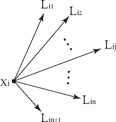
We define the Branch Length Similarity (BLS) entropy as the property of simple branching networks composed of n +1 nodes. Such a network is referred to as a Unit Branch Network (UBN) in this paper. Let xi be the position vector of the i-th node and Lij be the distance between xi and xj, such that Lij = |xi − xj|. For any i-th node, we consider the UBN as in Figure 1. The probability of the j-th branch of the i-th UBN is defined as Pij in Equation (1). By the mathematical form of the Boltzmann entropy, the BLS entropy, Si, of the i-th UBN is defined by:
2.1. Theoretical Results
Applying this notion to the nodes placed on an arbitrary bounded domain in ℝk for k ≥ 1, we obtain the following result.
Theorem 1. Let Ω be the bounded domain in ℝk for k ≥ 1. Suppose there are distinct (n +1) nodes in Ω. Then, the BLS entropy, Sn, of any node in Ω satisfies:
Assume that there are distinct n nodes in Ωn, except O. Letting Lj(j ≤ n) be the distance from O to each j-th node, it satisfies that ∊n ≤ Lj ≤ R. Hence:
Now, consider the second term of Equation (4). Since Lj ∈ [∊n, R], one has:
Theorem 1. can be extended to the unbounded domain in ℝk.
Corollary 1. Suppose that there are distinct (n +1) nodes on the unbounded domain, Ω, in ℝk. Then, the BLS entropy, Sn, of the node in Ω satisfies Equation (2).
Proof. All procedures of the proof are similar to Theorem 1.. Let ∊ and R be the shortest and longest distances from O to the other nodes, except O in Ω. Let Ωn = Ω ∩ {∊n < r < Rn} with and . Then, Ωn → Ω as n → ∞. Let Lj(j ≤ n) be the distance from O to each j-th node. Using ∊n ≤ Lj ≤ Rn and Equation (6), we can show that ln σ/ ln n → 1 as n →∞ by a similar way as Equation (5). Furthermore, limn→∞ δ/(σ ln n) = 0 by (ln ∊ +ln ln2 − ln ln n)σ ≤ δ ≤ (ln R +ln ln n − ln ln 2)σ. Thus, the required result follows by Equation (4).□
From Equations (4) and (5), the convergence rate behaves like:
2.2. Numerical Tests
We calculate the BLS entropies of the nodes on the bounded regions by increasing the number of nodes. To see the effect of the domain shape and the distribution of the nodes, we consider two regions (rectangle and triangle) and uniform and random distributions.
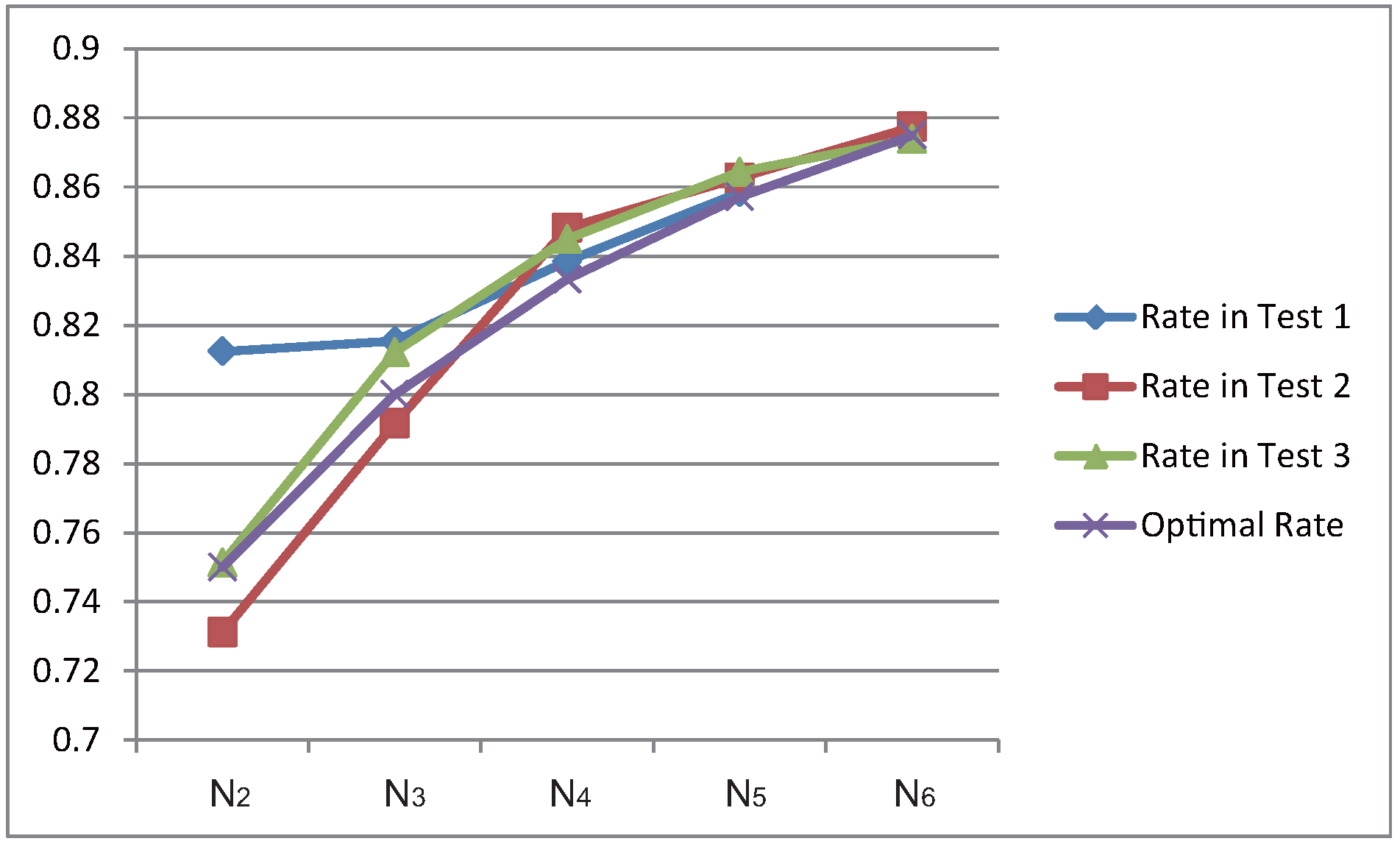
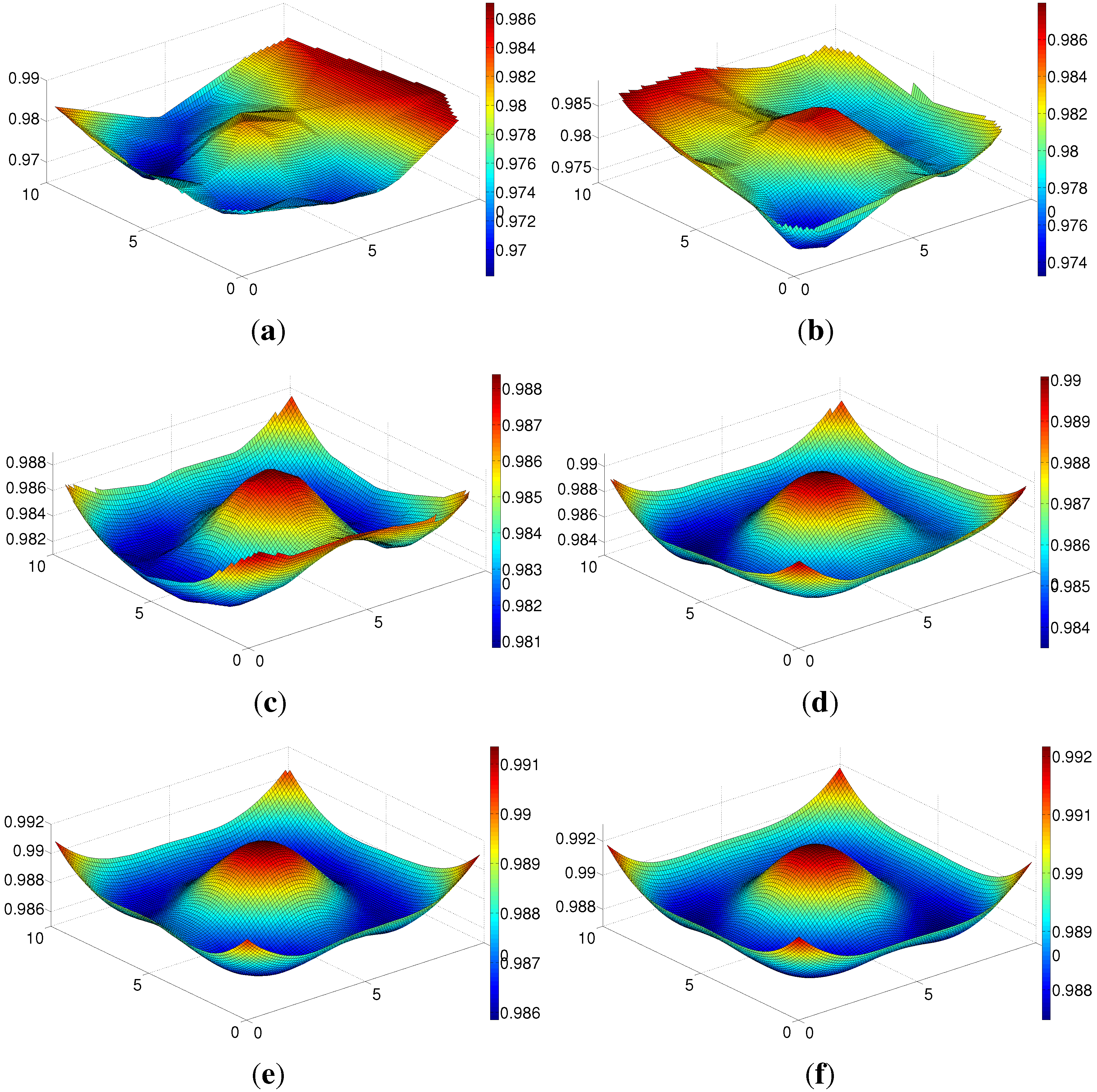
Test 1. First, consider the uniform network on the rectangle region R = [0, 10] × [0, 10]. Let M be a given natural number and h = 10/M. Dividing the rectangle region, R, by M2 squares, there are N ≔ (M +1)2 nodes on R, and the positions of the nodes are given by xij = (hi, hj) for 0 ≤ i, j ≤ M. For any (i, j)-th node, first, calculate the distances from the (i, j)-th node to others. Applying Equation (1), we obtain the BLS entropies for all nodes, and the BLS entropy profiles are drawn as Figure 2 for a given N. The local maximums are detected at the center and the four vertices. Since the BLS entropy grows up at the sharp corner, the local maximums occur at the vertices. The outlines of the profiles in Figure 2 are similar, but the interval of the BLS entropy grows up from N = 256 to N = 16, 384. To observe this behavior, we calculate the convergence rate in Table 1. Since the convergence rate is a log type, it converges slowly to one as N → ∞. Hence, we calculate the fractional order of the convergence rate by using the 2k nodes on the uniform network. In particular, we use N = 22n for an integer, n, since N is a square number. Here, |·|∞ is a L∞ norm, such that |v|∞ = supx∈R |v(x)|, and Rate denotes |1 − SNj|∞/|1 − SNj−1|∞. Optimal Rate, that is, the theoretical convergence rate by Equation (8), is defined by ln 22k/ ln 22(k+1) = k/(k +1). In Table 1, we can observe that Rate goes to Optimal Rate as N grows greater (see Figure 3). Thus, the convergence rate Equation (8) is confirmed.
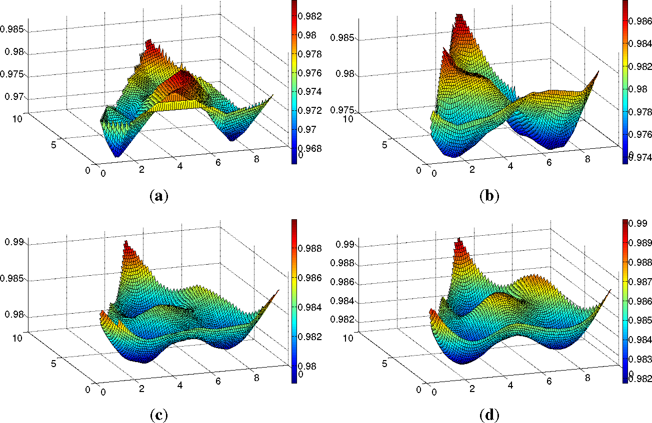
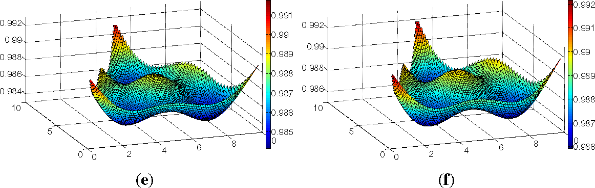
Test 2. Next is a result on the non-uniform network on the rectangle region, R. In this case, we spread the nodes randomly on R by the uniform distribution, that is, a symmetric probability distribution, whereby a finite number of values are equally likely to be observed; every one of the n values has equal probability 1/n. In the same way, we calculate the BLS entropies for all nodes. In this case, we take the mean value of the 10 times results in obtaining the norm, |1 − SN|∞, to reduce the effect of the randomness. For the ease of calculation, the convergence rate we set is the number of nodes N = 3k for an integer k. The figures in Figure 4 are depicted by using the interpolating method on the uniform grid (we used “griddata”, which is a built-in function of Matlab). For a small N, the profile of the BLS entropy has a complex shape, but the shape of the profile resembles the uniform case in Figure 2, as N is greater. By Figure 4 and Table 2, we can see that the interval of the profile grows up, and the convergence rate goes to Optimal Rate, though it is not as clear as Test 1 (see Figure 3).
Test 3. Next is the result of the non-uniform network on the triangular region, T, by spreading the nodes randomly using the uniform distribution. T is composed of three points, (0, 0), (10, 0) and (5, 10), and the BLS entropies of the nodes on T are calculated as in Figure 5. In this case, the local maximums are found at the center and three vertices and the profile are stable as N becomes greater. Its convergence rate also goes to Optimal Rate as N becomes greater.
3. Conclusions
In this paper, we showed that the BLS entropy of any network in ℝk increases at every node and, finally, converges to one as the number of nodes, N, increases, and we confirmed it by the numerical tests on the rectangle and triangle. Besides, the following relations are obtained by comparing Tests 1–3. From Tests 1 and 2, the different distributions of the networks on the same region do not effect the convergence rate for a sufficiently large N. Furthermore, the shape of the region has no effect on the convergence rate by Tests 2 and 3. However, the BLS entropy profile is characterized by the shape of the region. This is confirmed by Tests 1 and 2. Particularly, the BLS entropy profiles resemble each other as N increases.
One important point is: what is the optimal N in characterizing the shape of the region? Too small an N is likely to lose information regarding shape, while too large an N dilutes the characteristics of the region, since all entropies go to one as N →∞. Thus, finding the optimal number for N could provide positive support for the shape matching methods used and spreading the engineering applications.
Consequently, our result is meaningful in that it not only shows the convergence rate of the BLS entropy on the networks in ℝk, but also, it provides solid ground for the development of BLS entropy profile methods that could be practically used as a simple and useful tool for recognizing and characterizing shapes.
Acknowledgments
This work was supported by the National Institute for Mathematical Sciences.
Conflicts of Interest
The authors declare no conflicts of interest.
References
- Benda, L.; Poff, N.L.; Miller, D.; Dunne, T.; Reeves, G.; Pess, G.; Pollock, M. The network dynamics hypothesis: How channel networks structure riverine habitats. Bioscience 2004, 54, 413–427. [Google Scholar]
- Fisher, S.G. Creativity, idea generation, and the functional morphology of streams. J. N. Am. Benthol. Soc 1997, 16, 305–318. [Google Scholar]
- West, G.B.; Brown, J.H.; Enquist, B.J. A general model for the origin of allometric scaling laws in biology. Science 1997, 276, 122–126. [Google Scholar]
- Restrepo, J.G.; Ott, E.; Hunt, B.R. Emergence of coherence in complex networks of heterogeneous dynamical systems. Phys. Rev. Lett 2006, 96, 254103. [Google Scholar]
- Horton, R. Erosional development of streams and their drainage basins; hydrophysical approach to quantitative morphology. Geol. Soc. Am. Bull 1945, 56, 275–370. [Google Scholar]
- Schumm, S. Evolution of drainage systems and slopes in badlands ar perth amboy. N. J. Geol. Soc. Am. Bull 1956, 67, 597–646. [Google Scholar]
- Shreve, R. Stream lengths and basin areas in topologically random channel networks. J. Geol 1969, 77, 397–414. [Google Scholar]
- Strahler, A. Quantitative analysis of watershed geomorphology. Trans. Am. Geophys. Union 1957, 38, 913–920. [Google Scholar]
- Kirshen, D.; Bras, R. The linear channel and its effect on the geomorphologic IUH. J. Hydrol 1983, 65, 175–208. [Google Scholar]
- Arthur, W.B.; Holland, J.H.; LeBaron, B.; Palmer, R.; Tyler, P. The Economy as an Evolving Complex System II; Addison-Wesley: Boston, MA, USA, 1997. [Google Scholar]
- Lee, S.-H.; Su, N.-Y.; Bardunias, P. Novel approach to shape recognition using shape outline. J. Kor. Phys. Soc 2010, 56, 1016–1019. [Google Scholar]
- Kang, S.H.; Jeon, W.; Lee, S.-H. Butterfly species identification by branch length similarity entropy. J. Asia-Pac. Entomol 2012, 15, 437–441. [Google Scholar]
- Gaston, K.J.; May, R.M. Taxonomy of taxonomists. Nature 1992, 356, 281–282. [Google Scholar]
- Dale, M.R.T. Spatial Pattern Analysis in Plant Ecology; Cambridge University Press: Cambridge, England, 2000. [Google Scholar]
- Dale, M.R.T.; Zbigniewicz, M.W. Spatial pattern in boreal shrub communities: Effects of a peak in herbivore densities. Can. J. Bot 1997, 75, 1342–1348. [Google Scholar]
- Burrough, P.A. Spatial Aspects of Ecological Data. In Data Analysis in Community and Landscape Ecology; Jongman, R.H.G., Ter Braak, C.J.F., van Tongeren, O.F.R., Eds.; Cambridge University Press: Cambridge, England, 1995; pp. 213–251. [Google Scholar]
- Epperson, B.K. Spatial and space-time correlation in ecological models. Ecol. Model 2000, 132, 63–76. [Google Scholar]
- Anselin, L.; Florax, R.; Rey, S.J. Advances in Spatial Econometrics: Methodology, Tools and Applications; Springer-Verlag: Berlin, Germany, 2004. [Google Scholar]
- Anselin, L.; Syabri, I.; Kho, Y. GeoDa: An introduction to spatial data analysis. Geograph. Anal 2006, 38, 5–22. [Google Scholar]
- Jeon, W.; Lee, S.-H. Mathematical investigations of branch length similarity entrophy profiles of shapes for various resolutions. J. Kor. Phys. Soc 2012, 61, 1906–1910. [Google Scholar]


| N | |1 − SN|∞ | Rate | Optimal Rate |
| N1 = 82 = (23)2 | 2.6452E-2 | - | - |
| N2 = 162 = (24)2 | 2.1490E-2 | 0.81241 | 0.75000 |
| N3 = 322 = (25)2 | 1.7523E-2 | 0.81540 | 0.80000 |
| N4 = 642 = (26)2 | 1.4693E-2 | 0.83849 | 0.83333 |
| N5 = 1282 = (27)2 | 1.2613E-2 | 0.85844 | 0.85714 |
| N | |1 − SN|∞ | Rate | Optimal Rate |
|---|---|---|---|
| N1 = 34 | 3.3683E-2 | - | - |
| N2 = 35 | 2.4627E-2 | 0.73114 | 0.75000 |
| N3 = 36 | 1.9495E-2 | 0.79161 | 0.80000 |
| N4 = 37 | 1.6536E-2 | 0.84822 | 0.83333 |
| N5 = 38 | 1.4265E-2 | 0.86266 | 0.85714 |
| N6 = 39 | 1.2516E-2 | 0.87739 | 0.87500 |
| N | |1 − SN|∞ | Rate | Optimal Rate |
|---|---|---|---|
| N1 = 34 | 3.5863E-2 | - | - |
| N2 = 35 | 2.6943E-2 | 0.75128 | 0.75000 |
| N3 = 36 | 2.1883E-2 | 0.81220 | 0.80000 |
| N4 = 37 | 1.8489E-2 | 0.84490 | 0.83333 |
| N5 = 38 | 1.5982E-2 | 0.86441 | 0.85714 |
| N6 = 39 | 1.3968E-2 | 0.87398 | 0.87500 |
© 2014 by the authors; licensee MDPI, Basel, Switzerland This article is an open access article distributed under the terms and conditions of the Creative Commons Attribution license (http://creativecommons.org/licenses/by/3.0/).
Share and Cite
Kwon, O.S.; Lee, S.-H. Properties of Branch Length Similarity Entropy on the Network in Rk. Entropy 2014, 16, 557-566. https://0-doi-org.brum.beds.ac.uk/10.3390/e16010557
Kwon OS, Lee S-H. Properties of Branch Length Similarity Entropy on the Network in Rk. Entropy. 2014; 16(1):557-566. https://0-doi-org.brum.beds.ac.uk/10.3390/e16010557
Chicago/Turabian StyleKwon, Oh Sung, and Sang-Hee Lee. 2014. "Properties of Branch Length Similarity Entropy on the Network in Rk" Entropy 16, no. 1: 557-566. https://0-doi-org.brum.beds.ac.uk/10.3390/e16010557