Fully Bayesian Experimental Design for Pharmacokinetic Studies

Abstract

Utility functions in Bayesian experimental design are usually based on the posterior distribution. When the posterior is found by simulation, it must be sampled from for each future dataset drawn from the prior predictive distribution. Many thousands of posterior distributions are often required. A popular technique in the Bayesian experimental design literature, which rapidly obtains samples from the posterior, is importance sampling, using the prior as the importance distribution. However, importance sampling from the prior will tend to break down if there is a reasonable number of experimental observations. In this paper, we explore the use of Laplace approximations in the design setting to overcome this drawback. Furthermore, we consider using the Laplace approximation to form the importance distribution to obtain a more efficient importance distribution than the prior. The methodology is motivated by a pharmacokinetic study, which investigates the effect of extracorporeal membrane oxygenation on the pharmacokinetics of antibiotics in sheep. The design problem is to find 10 near optimal plasma sampling times that produce precise estimates of pharmacokinetic model parameters/measures of interest. We consider several different utility functions of interest in these studies, which involve the posterior distribution of parameter functions.

1. Introduction

1.1. Bayesian Experimental Design

The selection of optimal conditions for conducting experiments is crucial to maximise the worth of data, especially for situations in which experiments are costly and/or time consuming to conduct. Optimal experimental design aims to address these issues and may be employed to achieve the experimental goals in a more rapid and economical manner.

Experimental design has been well studied within the classical or frequentist framework, in both theory and practice (e.g., [1]). Classical optimal experimental designs are usually derived using optimality criteria that are based on the expected Fisher information matrix (e.g., [1,2]). Classical experimental design is well suited to linear or linearised models. However, for nonlinear models, designs are dependent on the model parameter values. Experimenters are often concerned with designing experiments to precisely estimate model parameters; so, the selection of the parameter values from which to construct the design is highly important, and the use of unsuitable parameter values may result in sub-optimal designs. In an attempt to obtain designs that are robust to the initial choice of parameter values, several studies (e.g., [3,4]) have incorporated probability distributions on the model parameters and averaged local design criteria over the distributions. These probability distributions are known as prior distributions and can incorporate information from previous studies, expert elicited data or subjective beliefs of the experimenters.

Bayesian methodologies for optimal experimental design have become more prominent in the literature (e.g., [5–10]). For an introduction to Bayesian experimental design, see Chaloner and Verdinelli [11]. Bayesian optimal design involves defining a utility function U(d, θ, y) that describes the worth (based on the experimental aims) of choosing the design d from the design space D yielding data y, with model parameter value θ. For example, the utility function could be the posterior precision of some parameter of interest. A probability model, p(θ, y|d), is also required. This consists of the likelihood p(y|d, θ) for observing a new set of measurements y at the design points d, given parameter value θ and a prior distribution p(θ) for the parameter θ.

The Bayesian optimal design, d*, maximises the expected utility function U(d) over the design space D with respect to the future data y and model parameter θ:

$$\begin{array}{l}\mathbf{d}*=\underset{\mathbf{d}\in \mathbf{D}}{\arg \max }E\{U(\mathbf{d},\theta ,\mathbf{y})\}\\ =\underset{\mathbf{d}\in \mathbf{D}}{\arg \max }{\displaystyle {\int }_{\mathbf{Y}}{\displaystyle {\int }_{\mathrm{\Theta }}U(\mathbf{d},\theta ,\mathbf{y})p(\theta ,\mathbf{y}|\mathbf{d})d\theta d\mathbf{y}}}.\end{array}$$

(1)

The integration is performed over the sample space Y of the data and the parameter space Θ. Unless the likelihood and prior are specifically chosen to enable analytic evaluation of the integration problem, Equation (1) does not usually have a closed form solution. Therefore, numerical approximations or stochastic solution methods are required to solve the maximisation and integration problem.

Fully Bayesian designs are those in which the design is obtained by using a design criterion that is a functional of the posterior distribution, such as the Kullback–Leibler distance [12] (between the prior and posterior [11]) or some function of the posterior variance (e.g., [13]). Designs that have arisen from averaging classical design criteria over the parameter space are termed “pseudo-Bayesian” or “robust” designs [4]. The fully Bayesian approach to optimal experimental design offers several advantages over the classical approach, the most significant of which is the ability to optimise design criteria that are functions of the posterior distribution and can easily be tailored to the experimental aims. Bayesian optimal design methods are often employed when the experimenter wishes to perform a Bayesian analysis of the data that is collected using the experimental design. The Bayesian approach also incorporates parameter uncertainties and prior information into the design process via prior distributions and provides a unified approach for joining these quantities with the model and design criterion. The Bayesian approach to design is especially important when the utility is not a standard one involving parameter estimation and when there is an informative prior, for example one based on earlier experiments. It is particularly important to incorporate the prior information into the parameter uncertainty assessment when experiments are being designed sequentially. The next design point can be chosen based on all available data to date in a sequential manner, with the posterior distribution being updated in a coherent manner. In a fully Bayesian experimental design, the prior information is combined with the data to form a posterior, and the utility is generally a function of the posterior. In a pseudo-Bayesian design the prior is used only to weight and average a functional of the Fisher information matrix.

1.2. Design of Pharmacokinetic Studies

Pharmacokinetic (PK) studies investigate the disposition of a drug following its administration to a subject or group of study subjects. PK studies generally assume that the change in drug concentration over time can be described by a particular model, such as a compartmental model. Compartmental models are usually derived by solving a series of ordinary differential equations, and error terms are incorporated into the model to account for any systematic or natural variation that may be present in the data. PK studies are often interested in measures, such as the area under the concentration-time curve (AUC), maximum concentration (C_max), time of maximum concentration (t_max), elimination half-life (t_1/2), clearance rate (CL) and the volume of the distribution (V) (e.g., [14–17]).

During PK studies, one cannot directly observe the kinetics of the drug in the study subjects, and so, samples are instead taken from biological fluids, such as blood, plasma or urine. These samples are taken at specific times, and the drug and metabolite concentrations are measured. The choice of plasma sampling times is highly important in PK studies. One should avoid complex designs that require a large number of samples to be taken from each study subject, since this would be costly and inconvenient for the study subjects. Thus, PK studies require the timing and number of samples to be carefully planned, so as to gain accurate estimates of the parameters, but also prevent physical and mental strain on the study subjects and reduce study costs.

Atkinson et al. [18] found designs that minimised the variance of the AUC, C_max and t_max estimates for an open one-compartmental PK model with first-order absorption input and a constant variance term. Prior distributions were used to account for parameter uncertainty. The designs found by Atkinson et al. [18] were c_θ -optimum and D_θ -optimum designs and were pseudo-Bayesian designs, since the utility functions were based on the Fisher information matrix. We will extend the results of Atkinson et al. [18] to enable fully Bayesian designs to be found for several of these PK parameters of interest.

1.3. Extracorporeal Membrane Oxygenation

Extracorporeal membrane oxygenation (ECMO) is a prolonged form of cardiopulmonary bypass and involves the diversion of blood flow through a circuit located outside of the body, so that the blood may be oxygenated. ECMO is used as a final resort in critically ill patients with potentially reversible respiratory failure to temporarily support the heart and/or lungs. In 2009, during the worldwide H1N1 pandemic, ECMO was a vital treatment modality for H1N1 patients requiring advanced ventilatory support [19–22] and has a reported survival rate of approximately 50% when used in critically ill adults with respiratory failure [23]. Despite the major benefits that ECMO can afford, it can also induce a wide variety of PK changes in critically ill patients that are not fully understood and can lead to therapeutic failure or toxicity. Thus, there is a need to understand the PK of critically ill patients undergoing ECMO.

1.4. Contribution and Outline

Optimal Bayesian experimental design involves sampling from the posterior distribution for many possible future datasets that are drawn from the prior predictive distribution. Therefore, many thousands of posterior distributions are required, and fast methods for approximating the posterior are necessary so that computation can be performed in a reasonable amount of time. Importance sampling has commonly been used in the literature to rapidly obtain samples from the posterior in the context of the Bayesian experimental design [6,24–27], where the prior is used as the importance distribution. However, importance sampling from the prior tends to break down and is inefficient if there is a reasonable number of experimental observations, since the posterior distribution can be very different from the prior. In this paper, we explore the use of the Laplace approximation for calculating Bayesian utility functions to overcome this drawback. Furthermore, we consider using the Laplace approximation to form the importance distribution to obtain a more efficient importance distribution than the prior.

The methodology is motivated by a PK study conducted by Shekar et al. [28], which investigates the effect of ECMO on the PK of antibiotics in sheep. Here, we will re-design their study to find 10 near-optimal plasma sampling times, which produce precise estimates of PK model parameters/measures of interest. In the PK study [28], healthy sheep had been administered the antibiotic, meropenem, and also underwent ECMO treatment. PK measurements were taken both before the sheep had undergone ECMO and after ECMO treatment had commenced, to determine the effect of ECMO on certain PK parameters of interest. We consider different utility functions in these studies, which involve posterior distributions of these PK parameters.

Whilst the algorithms we have borrowed from the Bayesian inference literature are not novel, to our knowledge, no previous works have investigated and compared the use of importance sampling and Laplace approximations for estimating the posterior in a Bayesian experimental design context. These estimates of the posterior are used to calculate Bayesian utility functions, some of which were specifically developed for our design problem of interest. Such a methodological investigation is necessary in order to advance the experimental design literature, so that optimal and fully Bayesian designs can be found when there is a large amount of data. The importance of this methodological development is highlighted by the ECMO application considered in this paper.

In Section 2, we introduce the motivating case study. Section 3 describes the utility functions used in this paper and the methods we use for estimating them. Our design methodology is outlined in Section 4, and our methods are applied to the case study in Section 5. The article concludes with a discussion in Section 6.

2. Case Study: Determining Sampling Times for a Study Investigating the Effects of ECMO on the PK of Meropenem in Sheep

Our design problem is based on a PK study conducted by Shekar et al. [28], in which healthy sheep were used as their own controls. Baseline PK data for meropenem (and other study drugs) were obtained from two healthy sheep, prior to commencing (venovenous) ECMO. Once ECMO began, 500 mg of meropenem (and the other study drugs) were infused over 30 min, and blood samples were taken at 0, 15, 30, 45, 60, 90, 120, 180, 360, 480 and 720 min after the commencement of the drug infusion. These blood samples were taken at the same time as the baseline PK measurements (when the sheep were not on ECMO). Here, we will be conducting a “retrospective study design” using existing PK data, to determine whether the study design can be improved upon for future studies.

It should be noted that our experimental design goal is to determine the 10 (near) optimal blood sampling times that give rise to precise estimates of PK parameters of interest. For reasons that will be clarified in Section 3, we are interested in using a somewhat large number of sampling times and are not concerned with reducing the number of observations taken. If one were interested in reducing the resources involved in the study, due to time or cost constraints, then one could investigate the optimal number of design points (e.g., [24,29]).

The data are assumed to be modelled by a one-compartment infusion PK model with fixed effects. This model does not account for individual variability, since our motivating case study only had data available for two sheep (which were very similar). The model has two parameters: the volume of distribution V, which is a theoretical volume that a drug would have to occupy to provide the same concentration as is currently present in the blood plasma (if the drug were uniformly distributed) and the first-order elimination rate constant k_e. If y_t denotes the observed concentration at time t min following the administration of the drug, then the model may be given by:

$$y_t=\{\begin{array}{ll}\frac{D}{T_{inf}}\frac{1}{k_{e}V}(1-e^{-k_{e}t})\cdot (1+{\epsilon }_t)& \mathrm{if}t\le T_{inf}\\ \frac{D}{T_{inf}}\frac{1}{k_{e}V}(1-e^{-k_e{T}_{inf}})e^{-k_e(t-T_{inf})}\cdot (1+{\epsilon }_t)& \mathrm{if}t>T_{inf},\end{array}$$

where ${\epsilon }_t\sim N(0,{\sigma }_{prop}^2)$, and t ∈ [0,720] min.

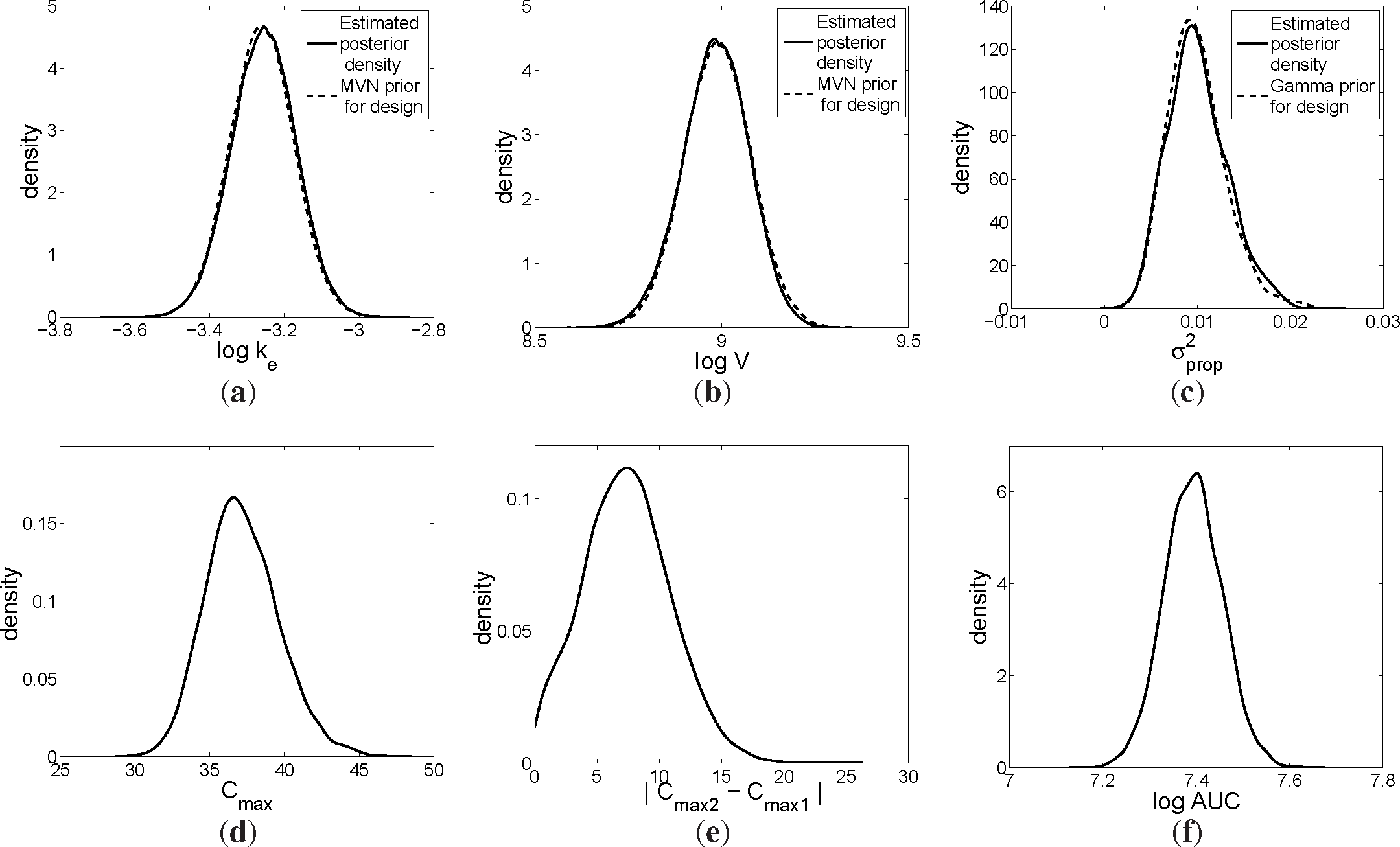
Here, the dose, D, is 500 mg, which was administered over a period of 30 min (i.e., T_inf = 30). Only proportional error (and not additive error) is present in the model. That is, the observational variance depends on the mean concentration at time t. This error structure gave a better fit to the data compared to models that contained only additive error, both additive and proportional error or exponential error. A Metropolis–Hastings Markov chain Monte Carlo (MH MCMC) algorithm was used to fit the above model to existing data for one of the sheep that underwent ECMO. The MCMC samples of the PK parameters that resulted from fitting the data to the model (Figure 1a,b) were used as the prior distributions for the retrospective design:

$$\theta \sim MVN\left\{\left(\begin{array}{c}-3.26\\ 8.99\end{array}\right),\left(\begin{array}{cc}0.0071& -0.0057\\ -0.0057& 0.0080\end{array}\right)\right\},$$

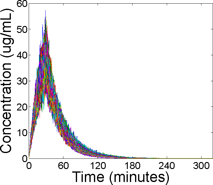
where θ = (logk_e, logV). Based on the MCMC samples (Figure 1c), ${\sigma }_{prop}^2$ was assumed to follow a gamma distribution with mean 0.01 and variance 10⁻⁵. ${\sigma }_{prop}^2$ was considered a nuisance parameter that was independent of k_e and V and was not of interest to estimate. The prior predictive curves of the data are displayed in Figure 2.

Here, our design points d are the sampling times t (in min), and we are searching for 10 (near) optimal sampling times in addition to t = 0.

3. Bayesian Utility Functions and Their Estimation

In this article, we investigate various design criteria that are concerned with the precise estimation of PK parameters. These design criteria are Bayesian and assume that a Bayesian analysis will be performed on any data that are generated from the experimental design. Bayesian utility functions are typically a scalar functional of the posterior p(θ |d, y), with expectation over the prior predictive distribution p(y|d, θ)p(θ). Thus, the prior is implicitly included in both the utility and the prior predictive distribution. In a recent article, Hainy et al. [30] review some fundamental results from Bayesian learning and provide a link to the optimal design of experiments by using functionals of Shannon information and functionals based on expected distance as utility functions.

Equation (1) does not typically have a closed form. Therefore, we will use Monte Carlo methods and/or Laplace approximations (described in Section 3.2) to approximate the posterior distribution. Once an approximation of the posterior has been obtained, it is typically straightforward to estimate the utility functions. For all of the utility functions mentioned in Section 3.1, we are interested in finding the optimal design d^* that maximises the expected utility function U(d) over the design space D, with respect to the unknown data y and model parameter θ.

3.1. Utility Functions

Each of the utility functions presented in this section are of the form:

$$U(\mathbf{d},\mathbf{y})={\{Var(\varphi |\mathbf{d},\mathbf{y})\}}^{-1},$$

where ϕ is some PK parameter of interest that will be defined below. That is, the utility functions consist of the posterior precision of some PK parameter of interest.

3.1.1. Posterior Precision of the Peak Concentration Estimate

Pharmacologists are often interested in determining the maximum concentration of a drug (C_max) in patients during PK studies to ensure that patients are not exposed to toxic concentrations (e.g., [14,16,17]). Here, our parameter of interest, ϕ, is the peak concentration estimate C_max, which occurs at the time when the infusion of the drug is complete (i.e., when t = T_inf). The expression for C_max is given by:

$$\varphi =C_{max}=y(T_{inf})=\frac{D}{T_{inf}}\frac{1}{k_{e}V}(1-e^{-k_e{T}_{inf}}).$$

(2)

For our case study, we decided to look at the C_max of meropenem for sheep receiving ECMO treatment. The posterior distribution of C_max that resulted from the MCMC fit to the data is displayed in Figure 1d.

3.1.2. Posterior Precision of the Difference in Peak Concentration Estimates Between Sheep on ECMO and Not on ECMO

Since pharmacologists are interested in determining the effect of ECMO on the PK curve [28], we decided to determine the (near) optimal design points that maximise the precision of the estimate of the difference in the concentration-time curve peaks for sheep on ECMO versus sheep not receiving ECMO treatment. Here, dϕ represents the absolute difference in the posterior peak concentrations for sheep not on ECMO and sheep on ECMO. The peak concentrations were calculated using Equation (2), and then, the absolute difference in the peaks was found:

$$\varphi =\left|C_{ma{x}_2}-C_{ma{x}_1}\right|=\left|\frac{D}{T_{inf}}\frac{1}{k_{e_2}{V}_2}(1-e^{-k_{e_2}{T}_{inf}})-\frac{D}{T_{inf}}\frac{1}{k_{e_1}{V}_1}(1-e^{-k_{e_1}{T}_{inf}})\right|,$$

where θ₁ = (logk_e1, logV₁) are the PK parameters for when the (one) sheep was on ECMO and θ₂ = (logk_e2, logV₂) are the PK parameters for when the (one) sheep was not on ECMO. The prior for θ₁ is given in Section 2. The prior for θ₂ that was obtained using the process outlined in Section 2 is:

$${\theta }_2\sim MVN\left\{\left(\begin{array}{c}-3.59\\ 8.94\end{array}\right),\left(\begin{array}{cc}0.0055& -0.0045\\ -0.0045& 0.0062\end{array}\right)\right\}.$$

The parameters θ₁ and θ₂ are assumed to be independent a priori. The posterior distribution of the absolute difference in C_max (between sheep on ECMO and sheep not on ECMO) that resulted from the MCMC fit to the data is displayed in Figure 1e.

3.1.3. Posterior Precision of the (Log) AUC Estimate

Pharmacologists are also interested in estimating the AUC for concentration-time curves to determine the patients’ total exposure to a drug (e.g., [14–17]). To enable an analytic solution to be found for the precision of the posterior distribution of this parameter of interest (when using Laplace approximations to approximate the posterior distribution), we decided to instead look at the log AUC, which was closer to being normally distributed a priori than the (non-transformed) AUC. Here, ϕ represents the log AUC. Since we have a (simple) one-compartment PK model, we can find the log AUC analytically, by logAUC = logD − logk_e − logV. Therefore,

$$\varphi =\log D-\log k_e-\log V.$$

For our case study, we decided to look at the log AUC of meropenem for sheep receiving ECMO treatment. The posterior distribution of the log AUC that resulted from the MCMC fit to the data is displayed in Figure 1f.

3.1.4. Determinant of the Posterior Precision Matrix

If one is interested in designing for the precise estimation of the elimination constant logk_e and the volume of distribution logV, then one could use the determinant of the posterior precision matrix of the PK model parameters as the utility function. Here, ϕ = (logk_e, logV). The determinant of the posterior precision matrix of the model parameter is also known as the “Bayesian D-posterior precision” [13]. This utility is estimated by finding the determinant of the precision matrix of the θ sample from the posterior. For our case study, we looked at precisely estimating logk_e and logV for sheep receiving meropenem and on ECMO treatment.

3.2. Methods for Estimating Utility Functions

Each of the above-mentioned utility functions requires the posterior distribution p(θ|d, y). However, the posterior often does not have a closed form expression, and so, numerical methods are required to sample from or approximate the posterior distribution. Each possible future dataset that is drawn from the prior predictive distribution requires calculations of the posterior distribution, and so, many thousands of posterior distributions need to be considered. Hence, fast methods for obtaining the posterior distribution are required. In this paper, we explore, compare and contrast importance sampling and Laplace approximations for this purpose.

3.2.1. Importance Sampling

Importance sampling is a commonly-used approach for approximating target distributions of interest [31]. It involves choosing an alternative distribution g(·) (the importance distribution), from which it is easy to sample, then appropriately weighting the samples to account for the discrepancy between g(·) and the target distribution. Here, the target distribution is the posterior p(θ|y, d). This produces weighted samples ${\{{\theta }_k,W_k\}}_{k=1}^{M_p}$, where M_p is the number of particles used to approximate p(θ|y, d), $w(\theta )=\frac{p(\mathbf{y}|\theta ,\mathbf{d})p(\theta )}{g(\theta )}$ are the importance weights and W_k ∝ w(θ_k) are the normalised importance weights, ${\displaystyle {\sum }_{k=1}^{M_p}{W}_k=1}$. The distributions p(θ|y, d) and g(θ) should have the same support. A common approach in Bayesian experimental design is to use the prior as the importance distribution g(θ) = p(θ) (e.g., [6,24,27]), and the importance weights are reduced to the likelihood function. However, this can be very inefficient for diffuse priors [32] or concentrated likelihoods, which result here from having a large number of observations.

To measure the efficiency of importance sampling, the effective sample size (ESS) is used, where:

$$\mathrm{ESS}=\frac{1}{\Sigma W_k^2},1\le \mathrm{ESS}\le M_p.$$

The utility functions presented in Section 3.1 were estimated using the sample weighted variance that was estimated using the importance weights given by the likelihood function, since the prior was used as the importance distribution (see [17] for further details). For each of these utility functions, the proportional variance ${\sigma }_{prop}^2$ was only used to calculate the importance weights and was not one of the parameters of interest that we were designing to precisely estimate.

In our applications, the number of particles M_p was chosen to ensure that reasonably stable (based on the ESS) and precise estimates of the utility were obtained. For each iteration of the MCMC algorithm that was used (see Section 4.2), the M_p value was increased until an ESS value of 1000 or more was obtained, so that the utilities could be estimated using at least the equivalent of 1000 independent samples from the posterior. We conducted a sensitivity analysis into this minimum value of the ESS and found that values less than 1000 tended to give less precise estimates of the utility and did not provide a good exploration of the design space, as the MCMC design search algorithm would become “stuck” at a particular design when its corresponding utility was over-estimated.

When the determinant of the posterior precision matrix was used as the utility function, a large number of samples was often required to ensure an ESS value of 1000. However, an upper bound of M_p = 100 million had to be set, as larger values than this caused memory storage issues. Therefore, some of the samples that were used to calculate this utility function had an ESS value less than 1000. This highlights the difficulty of using the prior as the importance distribution for designs with a reasonable number of observations.

Importance sampling from the prior is usually inefficient for large amounts of data, since the posterior distribution can be very different from the prior. Although reducing the number of observations taken would improve the performance of importance sampling, this lies outside the scope of the current study, as we are not concerned with time or cost constraints. In this study, we are interested in comparing the performance of importance sampling to other methods for approximating the posterior distribution (see below) for design problems where (somewhat) large amounts of data are involved.

3.2.2. Laplace Approximation

It is widely known that Monte Carlo methods, such as importance sampling, may fail in cases where large amounts of data are involved (e.g., [27,33]). To overcome this, we suggest the use of Laplace approximations to the posterior distribution of θ (suitably parameterised), instead of importance sampling. Laplace approximations have previously been used in the PK design literature (e.g., [34,35]) to solve the integrals involved in the expected Fisher information matrix. Here, the Laplace approximation assumes a multivariate normal distribution for the posterior distribution of the parameter θ, as well as log ${\sigma }_{prop}^2$. One simply uses a numerical search algorithm, such as a quasi-Newton method, to estimate the posterior mode:

$$(\widehat{\theta },\log {\widehat{\sigma }}_{prop}^2)=argma{x}_{\theta \in \mathrm{\Theta },\log {\sigma }_{prop}^2\in \Re }\log p(\theta ,\log {\sigma }_{prop}^2|\mathbf{y},\mathbf{d}),$$

and the posterior variance-covariance matrix (of θ) via the upper-left quadrant of −1 times the inverse of an estimate of the Hessian matrix evaluated at the $(\widehat{\theta },\log {\widehat{\sigma }}_{prop}^2)$ value. The approximation can be used directly (as we do for the Bayesian D-posterior precision utility), or samples can be drawn from this Gaussian approximation to estimate quantities that are functions of the model parameters (e.g., C_max).

It is important to note that use of the Laplace approximation relies on the assumption that the posterior distribution of the parameter θ is reasonably well approximated by a multivariate normal distribution. If this assumption is not valid, then use of Laplace approximations to estimate the posterior distribution may not be appropriate. Laplace approximations also suffer from the curse of dimensionality. To overcome this issue, Long et al. [36] used polynomial-based sparse quadrature to integrate over the prior distribution. Furthermore, the estimated posterior distribution obtained from the Laplace approximation may not accommodate the tails of the posterior distribution, and so, we investigate alternative methods to obtain better coverage of the tails.

3.2.3. Importance Sampling with a More Informed Importance Distribution (“Combined Approach”)

To improve the efficiency of the prior as the importance distribution (which may be too diffuse), we considered the use of the Laplace approximation to form the importance distribution. This approach was proposed by Kuk [37] in a Bayesian inference framework to estimate the likelihood function of generalised linear mixed models (GLMMs). Kuk [37] stated that since the Laplace approximation is only used to suggest an appropriate importance distribution, the accuracy of the Laplace approximation affects only the efficiency and not the unbiasedness of the resulting likelihood estimate. To our knowledge, this approach has not been used in the Bayesian design framework to approximate the posterior distribution for Bayesian utilities.

To obtain better coverage of the tails (than the Laplace approximation), we multiplied the variance-covariance matrix that was obtained from the Laplace approximation by two, drew many samples from the multivariate normal distribution, calculated quantities, such as the AUC or C_max and then weighted these samples by the importance weights. This approach may also account for any non-normality in the posterior distribution. The importance weights were calculated in a similar manner to Section 3.2.1, but with one major difference: in Section 3.2.1, the importance distribution g(θ) was the prior distribution, but for the combined approach, the importance distribution was the multivariate normal density, which resulted from the Laplace approximations.

3.2.4. Other Methods

Previous approaches, such as Han and Chaloner [7], have used MCMC to approximate the posterior distribution for the utility function calculations. However, Han and Chaloner [7] only investigated fixed designs, and no optimisation was performed over the design space. Whilst MCMC is useful and often appropriate for Bayesian data analysis, it may not be suitable for optimal Bayesian experimental design, as it is computationally intensive to perform MCMC to approximate the posterior distribution for each of the thousands of iterations required in the Bayesian experimental design algorithms. For importance sampling, the precision of the algorithm can be controlled by using the ESS. An ESS is more difficult to determine for MCMC; a burn-in period is required, and so, it is more difficult to automate; and various tests are required to determine the convergence of the MCMC algorithm. For these reasons, we did not investigate the use of MCMC to approximate the posterior distributions required to perform the Bayesian experimental design.

We note that a multivariate t-distribution with a small number of degrees of freedom could be used in place of the multivariate normal distribution for the importance distribution in the “combined approach” to obtain a wider coverage of the tails. However, we found our approach (where the variance-covariance matrix of the multivariate normal distribution is twice the value of the variance-covariance matrix obtained from the Laplace approximation) to be sufficient for our motivating application.

4. Design Methodology

4.1. Stochastic Optimisation

One of the most commonly-used stochastic algorithms for solving the maximisation and integration problem (Equation (1)) involves the use of Monte Carlo simulations to evaluate the integral(s) (Equation (1)) (e.g., [9,38]). In the majority of situations, p(θ, y|d) is available for efficient random variable generation, and the utility function can be evaluated point-wise using the simulated (θ_i, y_i) for i = 1, …, M. The integral may then be approximated by using:

$$\widehat{U}(\mathbf{d})=\frac{1}{M}{\displaystyle \sum _{i=1}^{M}U(\mathbf{d},{\theta }_i,{\mathbf{y}}_i)}.$$

(3)

One can then use Û(d) to find the optimal design, d* = arg max Û(d), by using a suitable maximisation method (see [9]). However, straightforward Monte Carlo integration over (θ, y) for each design d can be computationally intensive for design problems involving a large number of design variables, since the design space grows far too rapidly with the number of design variables, and thus, the search over the design space becomes infeasible. Furthermore, when a design variable corresponds to a data point, then a larger number of design variables means that more observations are involved, which implies a larger integral over y, and thus, a larger value of M is required to accurately estimate U(d).

Instead, Müller and colleagues [9,39,40] performed the integration using MCMC, which sampled from the target distribution:

$$h(\mathbf{d},\theta ,\mathbf{y})\propto U(\mathbf{d},\theta ,\mathbf{y})p(\theta ,\mathbf{y}|\mathbf{d})$$

using an MH MCMC scheme. It was assumed that U(d, θ, y) satisfies the appropriate conditions for h(·) to be positive and integrable over (D, Θ, Y). The probability distribution h(·) is defined such that the marginal distribution of d is proportional to the expected utility, U(d). The MCMC simulation focuses on sampling in areas of high expected utility and discourages sampling in areas of low expected utility (see [9]). The sample of simulated d may be used to provide an estimate of h(d), and the joint mode of h(d), d*, corresponds to the optimal design.

A “simulated annealing-type approach” (see [9,39–41]) has also been suggested, in which a sample is simulated from:

$$h_J(\mathbf{d},{\theta }_1,\dots ,{\theta }_J,{\mathbf{y}}_1,\dots ,{\mathbf{y}}_J)\propto {\displaystyle \prod _{j=1}^{J}U(\mathbf{d},{\theta }_j,{\mathbf{y}}_j)p({\theta }_j,{\mathbf{y}}_j|\mathbf{d})}.$$

The marginal h_J(d) is proportional to U^J(d), where J is an integer. As J increases, the utility surface will become more peaked, and simulations will cluster more tightly around the mode.

Alternative simulation-based algorithms for maximising the expected utility, such as sequential Monte Carlo (see [5]), have also been proposed. However, we found the MCMC approach of Müller and colleagues [9,39,40] to be sufficient for sampling the design space for our design problems.

4.2. MCMC Algorithm

To solve the optimal design problems (Equation (1)), we implemented the MH MCMC algorithm presented by Müller [9], which is described in

Algorithm 1:. Markov chain Monte Carlo (MCMC) algorithm for Bayesian optimal design [9]. MH = Metropolis–Hastings.

1	Initialise: set an initial design d(1), simulate (θj, yj) from p(θ, y|d(1)) = p(θ)p(y|d(1), θ) for j = 1, …, J
2	Compute $U^{(1)}={\displaystyle {\prod }_{j=1}^{J}U({\mathbf{d}}^{(1)},{\theta }_j,{\mathbf{y}}_j)}$ U(d(1) θj, yj)
3	for i = 1 to iters do
4	Generate a candidate design $\tilde{\mathbf{d}}\sim q(\cdot |{\mathbf{d}}^i)$, propose $({\tilde{\theta }}_j,{\tilde{\mathbf{y}}}_j)\sim p(\theta ,\mathbf{y}|\tilde{\mathbf{d}})=p(\theta )p(\mathbf{y}|\tilde{\mathbf{d}},\theta )$ for j = 1, …, J
5	If $\tilde{\mathbf{d}}$ is not within the design space, then reject the proposal and go to Line 9
6	Compute $\tilde{U}={\displaystyle {\prod }_{j=1}^{J}U(\tilde{\mathbf{d}},{\tilde{\theta }}_j,{\tilde{\mathbf{y}}}_j)}$
7	Calculate the MH acceptance probability, a = min(1, A), where
	$A=\frac{\tilde{U}\times q({\mathbf{d}}^{(i)}|\tilde{\mathbf{d}})}{U^{(i)}\times q(\tilde{\mathbf{d}}|{\mathbf{d}}^{(i)})}$
	Here, U(i) and d(i) are the current utility and design point values, respectively, and Ũ and $\tilde{\mathbf{d}}$ are the proposed utility and design point values, respectively.
8	Set $({\mathbf{d}}^{(i+1)}),(U^{(i+1)})=(\tilde{\mathbf{d}},\tilde{U})$ with probability a and
9	(d(i+1), U(i+1)) = (d(i), U(i)) with probability 1 − a.

in the Online Resources (Appendix A), to perform simulation from h(·). We found that J = 5 provided sufficiently peaked utility surfaces for our design problems. The methods described in Section 3.2 were used in Lines 2 and 6 of Algorithm 1 in the Online Resources (Appendix A) to estimate the posterior distribution for use in the Bayesian utility function calculation.

We note that the joint mode of h(d) needs to be found rather than the marginal modes for each element of d, as the latter may be very different from the former.

MCMC runs of 10,000 iterations were performed, and the convergence of the algorithms was carefully monitored (through examination of autocorrelation plots, histograms and contour plots of the design variables and trace plots of the utility functions over the iterations). The prior distribution was used as the proposal distribution for the model parameter, and the design variables were proposed from a normal random walk. To determine the optimal designs, we searched for the multivariate mode of the multivariate normal kernel smoothing density estimates of the design variables (see [6,42]).

4.3. Lower Dimensional Parameterisations

Here, we use an approach from our previous work [27] that reduces the computational burden of searching for a large number of design points. This approach involves the use of lower dimensional parameterisations that consist of a few design variables, which generate multiple design points. Using this approach, one simply has to search over a few design variables, rather than searching for a large number of optimal design points, thus providing substantial computational savings. The following lower dimensional parameterisation schemes were used to generate the design points:

• d_s = d₁ δ ^(s−1), where d₁ ≥ 0, δ > 1 (“geometric scheme”);
• d_s = d₁ +δ × (s − 1), where d₁ ≥ 0, δ > 0 (“even spacing scheme”); and
• Percentiles of a Beta(a, b) distribution, scaled to [0,T]—the design space, where a, b > 0 (“beta scheme”).

Here, d₁ is the first design point, δ is a spacing parameter, (a, b) are positive shape parameters for a beta distribution, s is an index where s = 1, …, n_d and n_d is the number of design points. Under these lower dimensional parameterisations of the design points, the Müller [9] algorithm searched over two design variables (d₁, δ) or (a, b), depending on the scheme that was used. This avoids the need to search for a large number of optimal design points and provides substantial computational savings. Furthermore, it is much easier to obtain the multivariate mode for a few design variables than for a large number of design variables. However, it should be stressed that the designs generated by the lower dimensional parameterisations are not optimal, but near-optimal, which is a compromise of the computational savings achieved through these methods.

A typical experimental design for PK studies where the drug concentration-time profile is thought to be modelled by a compartmental model is the geometric design (“geometric scheme” above) [18]. We also decided to investigate the use of evenly-spaced designs and designs that arose from the (evenly-spaced) percentiles of the beta distribution, as we thought that these schemes may give fairly flexible designs that could be suitable for use in PK studies.

For comparative purposes, we also searched for optimal designs for a three design (support) point problem using the Müller [9] algorithm, where the design variables were (d₁, d₂, d₃), i.e., the three sampling times for the PK study. This involved searching for three optimal sampling times, which were generated in the MH MCMC algorithm via normal random walks and did not involve the use of the lower dimensional parameterisation schemes. Once these three sampling times were determined, replicates were placed on each of these support points, so that a total of 10 design points were obtained (four replicates on d₁, three replicates on d₂, three replicates on d₃). Since true replication is not practically feasible for a PK study, these ‘replicates’ were separated by a time interval of 15 min.

Following the dimension reduction of the design problem (to two design variables), a brute force approach was also investigated, in which the expected utility was calculated using Monte Carlo integration (Equation (3)), and optimisation was performed by searching over a grid of values for the design variables (e.g., [43]). However, the brute force approach was found to be too computationally intensive, and it was difficult to determine an appropriate grid of values to encompass regions of high expected utility for our applications of interest. Therefore, results will not be discussed for this method.

All simulations were performed on an Intel Xeon Processor E5-2670 (2.66 GHz, 1 GB RAM).

5. Results

The utility function values for the optimal designs (Figures 3–6) were calculated using Monte Carlo integration (Equation (3)) with M = 1000. The Monte Carlo sample size was chosen to ensure that the 95% CIs were accurate to two decimal places. Figures 3–6 appear in colour in the online version of this article.

In general, the estimates of the utility functions were quite similar across the three methods for calculating the utilities (see Figures 3–6). The run times for the different utilities varied significantly across the three methods in most cases (see

Table 1. Run times (min)^a for the different methods for calculating the utility functions for when the geometric scheme was used to generate the designs. Here, U₁ = posterior precision of C_max; U₂ = posterior precision of the difference in C_max for ECMO vs. non-ECMO; U₃ = posterior precision of log AUC; and U = det(posterior precision). ^aThese run times are based on MCMC runs of 10,000 iterations.

Method for estimating utility function	U1	U2	U3	U4
Importance sampling	59	362	44	85
Laplace approximation	2	5	2	1
Combined approach	10	91	7	23

), with the Laplace approximation being the fastest, followed by the combined approach and then importance sampling (from the prior). In particular, the run times for the posterior precision of the absolute difference in peak concentration estimates for sheep on ECMO vs. sheep not on ECMO utility (U₂(d, y)) were much slower for importance sampling compared to the other methods. This is due to the fact that importance sampling required a larger number of particles to provide a stable estimate of the utility. The importance sampling run time for the Bayesian D-posterior precision utility could have been just as slow (if not slower) if no upper bound on M_p were present.

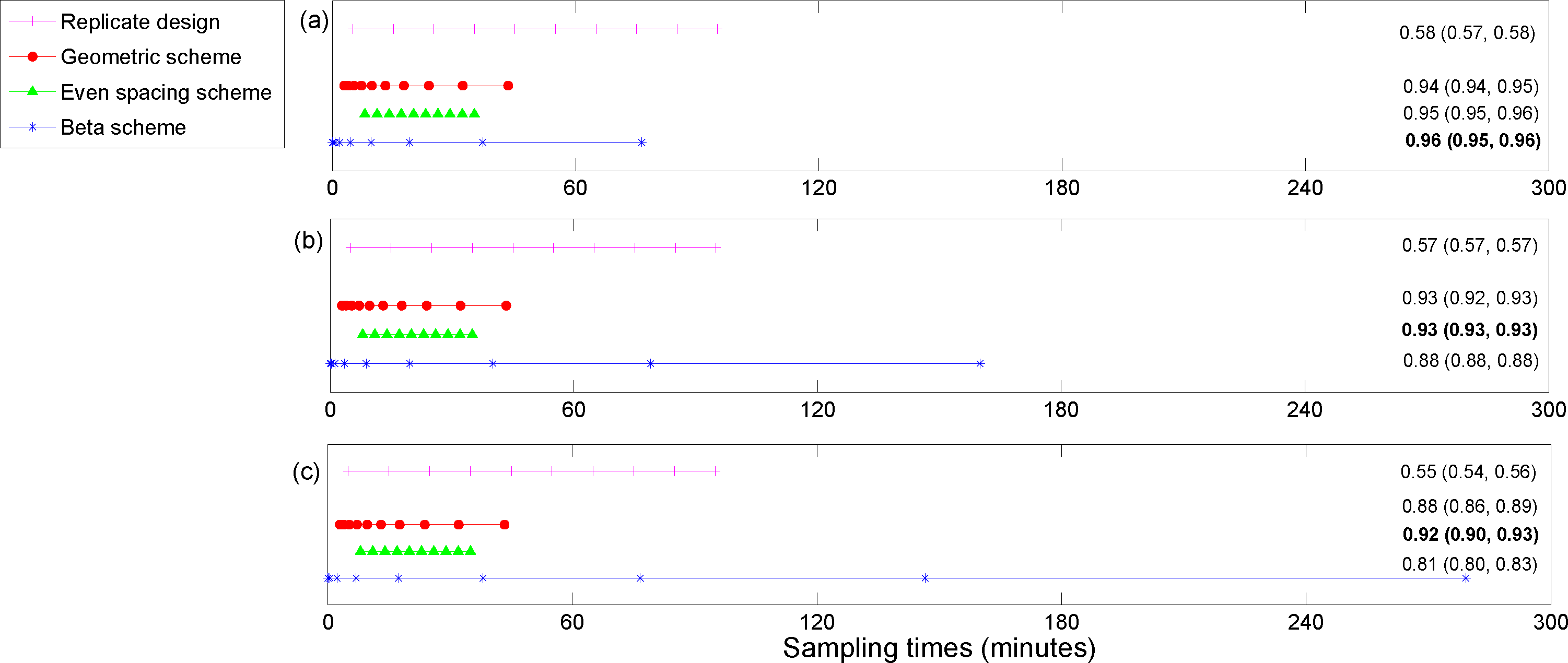
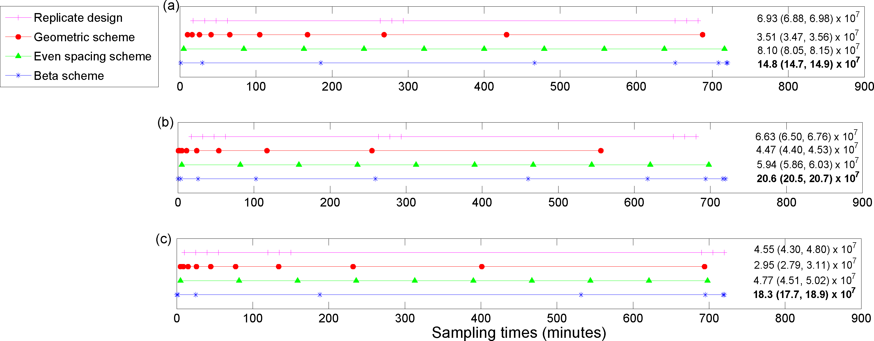
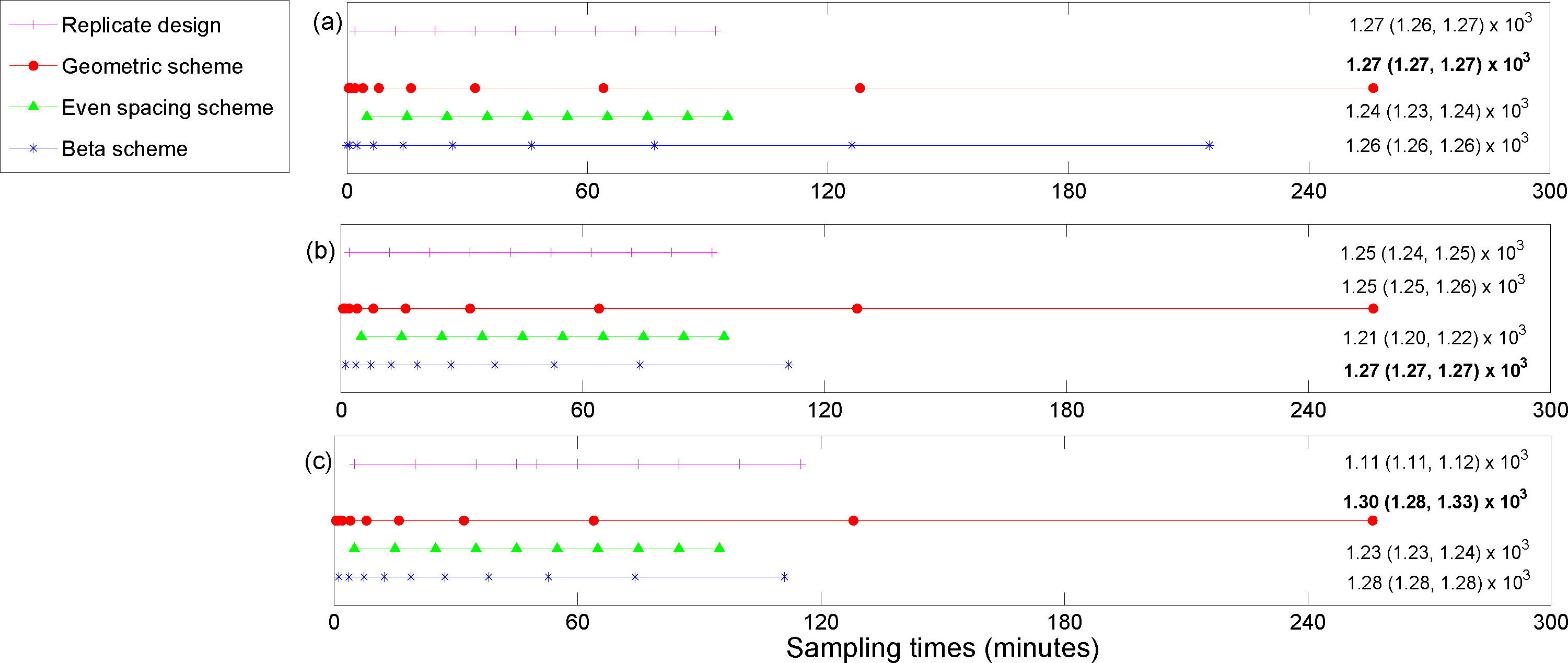
For the posterior precision of C_max and the posterior precision of the difference in C_max for ECMO vs. non-ECMO utility functions, the designs were quite similar across the three methods for estimating the utility functions. Sampling was mostly focused around the peak concentration (the beta scheme and, occasionally, the replicate designs also sampled beyond these times). For the posterior precision of the log AUC utility, the designs mostly focused on sampling in areas where the concentration was non-zero and were quite similar across the three methods for estimating the utilities. However, the geometric scheme covered a greater area of the concentration-time curve and also sampled where the concentrations were approximately zero. The designs that were generated for the determinant of the posterior precision matrix utility function were similar across the three methods and covered the majority of the sampling space. The beta scheme produced the optimal designs for this utility, and the beta distribution was in the shape of a “bath tub” curve over the design space. The original sampling times that were used by Shekar et al. [28] were always outperformed by the optimal designs that were found in this paper, for our utility functions of interest (see the captions for Figures 3–6). This highlights the importance of these methods for determining an optimal experimental design.

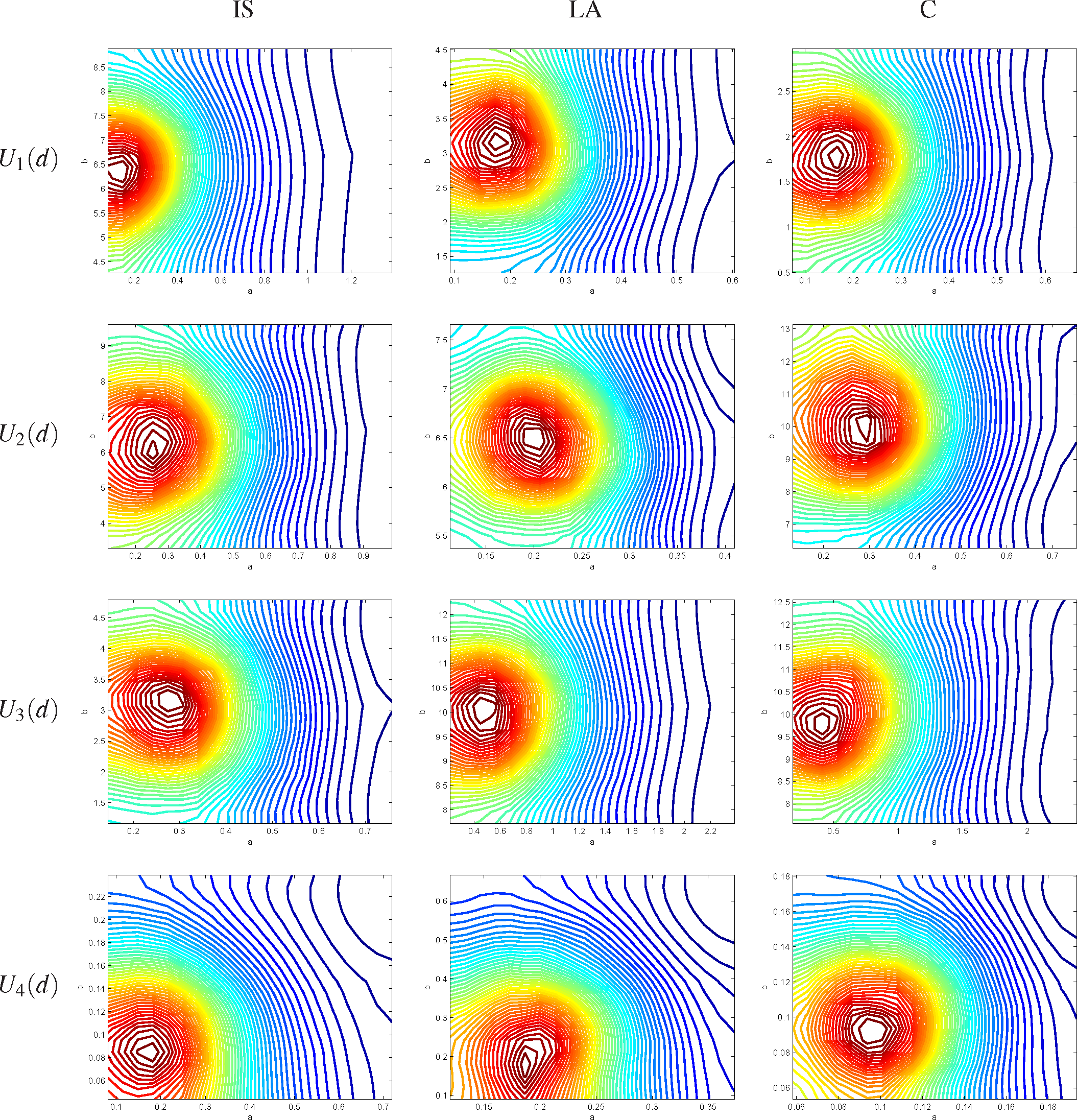
Contour plots of the posterior samples of the beta scheme design variables (a, b) for each of the utility functions and methods of calculating the utilities are displayed in Figure C1 in the Online Resources (Appendix C).

For each of the utility functions, the beta scheme was often found to perform quite well across the three methods for calculating the utilities. Therefore, it was decided to perform a comparison of the (optimal) designs generated by the beta schemes across the different utility functions and methods for calculating the utilities, to see how these designs differed. A graphical comparison of the beta scheme designs is displayed in Figure B1 in the Online Resources (Appendix B).

A quantitative comparison was performed, in which the beta scheme design from one utility function was input into the other three utility functions, and their values were calculated. A ratio was then calculated in which these utility function values were compared to the values of those utility functions evaluated at their own beta scheme designs (Columns 4–7 in

Table 2. Comparison of the optimal beta proposal scheme designs for each utility function evaluated at the other utility functions, across the different methods for calculating the utilities. U_Orig is the utility function that the beta scheme design originally came from; (a, b) are the values of the shape parameters for the beta scheme; $R_{U_1}$, $R_{U_2}$, $R_{U_3}$ and $R_{U_4}$ are the values of the utilities (with 95% CI in brackets) evaluated at the beta scheme design, which came from the utility U_Orig divided by the utility evaluated at its own beta scheme design (ratios). Here, U₁ = posterior precision of C_max; U₂ = posterior precision of the difference in C_max for ECMO vs. non-ECMO; U₃ = posterior precision of log AUC; and U₄ = det(posterior precision); IS = importance sampling; LA = Laplace approximation; and C = combined approach.

Method	UOrig	(a, b)	$R_{U_1}$	$R_{U_2}$	$R_{U_3}$	$R_{U_4}$
IS	U1	(0.21, 6.55)	–	0.91 (0.91, 0.92)	0.72 (0.71, 0.72)	0.09 (0.09, 0.10)
	U2	(0.3, 6.2)	0.95 (0.94, 0.95)	–	0.93 (0.93, 0.94)	0.03 (0.03, 0.04)
	U3	(0.3,3)	0.83 (0.83, 0.84)	0.98 (0.98, 0.99)	–	0.04 (0.04, 0.05)
	U4	(0.2, 0.1)	0.43 (0.43, 0.43)	0.82 (0.82, 0.82)	0.46 (0.45, 0.47)	–
LA	U1	(0.2, 3)	–	0.93 (0.93, 0.94)	1.02 (1.01, 1.02)	0.02 (0.02, 0.02)
	U2	(0.21, 6.55)	1.08 (1.07, 1.08)	–	0.64 (0.63, 0.65)	0.01 (0.01, 0.01)
	U3	(0.6, 10)	0.92 (0.91, 0.93)	0.84 (0.84, 0.85)	–	0.01 (0.01, 0.01)
	U4	(0.2, 0.2)	0.60 (0.60, 0.61)	0.57 (0.56, 0.58)	0.59 (0.59, 0.60)	–
C	U1	(0.2, 1.7)	–	0.92 (0.92, 0.92)	1.03 (1.02, 1.03)	0.31 (0.31, 0.32)
	U2	(0.3, 10)	1.07 (1.06, 1.07)	–	0.90 (0.90, 0.91)	0.29 (0.29, 0.30)
	U3	(0.6, 10)	1.02 (1.02, 1.03)	0.91 (0.90, 0.91)	–	0.29 (0.28, 0.30)
	U4	(0.1, 0.1)	0.80 (0.80, 0.81)	0.72 (0.72, 0.73)	0.99 (0.98, 0.99)	–

).

The majority of the utility functions performed quite well (as indicated by high ratios) when designs from other utility functions were input. The exception to this was that when the designs from the other three utilities were input into the determinant of the posterior precision matrix utility, low ratio values were obtained for all three methods of estimating the utility. This is not surprising given how different the designs obtained for the determinant of the posterior precision matrix utility were compared to the designs obtained for other utility functions (see Figures 3–6). These results suggest that this utility function is not robust to design objective uncertainty, and if one is interested in precisely estimating all PK model parameters, then one should specifically design the experiment to do so and not rely on other designs.

6. Discussion

In this paper, we have compared and contrasted three methods for calculating Bayesian utility functions: importance sampling using the prior as the importance distribution; Laplace approximations; and importance sampling using the Laplace approximation to the posterior as the importance distribution. These approaches to calculating the utility functions were incorporated into an MCMC algorithm, which searched for the (near) optimal design for a PK study, which required 10 plasma sampling times to be found. Four Bayesian utility functions were used, which focused on precisely estimating various PK measures of interest and were functions of the PK parameters.

The optimal designs that were found differed substantially between the utility functions, but were fairly similar between the different methods for calculating the utility functions (for a given utility function). The posterior precision of C_max, the posterior precision of the difference in C_max for ECMO vs. non-ECMO and the posterior precision of the log AUC utility functions were found to be fairly robust to uncertainty in the design objectives. However, the determinant of the posterior precision matrix utility was not found to be robust to design objective uncertainty. This means that designs that are generated by other utility functions should not be used if one is interested in precisely estimating all PK model parameters.

The Laplace approximation method was generally found to be the fastest of the three methods. The combined approach was computationally faster than the importance sampling (from the prior) approach, since fewer importance samples were required to obtain stable and precise estimates of the utilities. When importance sampling was used to estimate the utility functions, many importance samples were required to obtain reasonable ESS values. Both the Laplace approximations and the “combined approach” were able to produce similar results to brute force importance sampling, but in a more timely manner. This is of high importance when one is interested in designing experiments that involve large amounts of data to be collected.

The use of each of these methods for approximating the posterior distribution is problem dependent. Previously, importance sampling from the prior has been used as a gold standard (e.g., [6,27]). However, if large amounts of data are involved, then we do not recommend the use of importance sampling from the prior distribution, as this method was found to be computationally intensive, due to the large number of particles required to obtain a reasonable ESS. The Laplace approximation approach is useful when large amounts of data are involved, but its suitability depends on whether it is reasonable to assume that the posterior distribution follows a multivariate normal distribution. This could be a reasonable assumption in many design applications where large amounts of data are involved and/or if the priors are reasonably informative. If the Gaussian assumption is not reasonable, then we do not recommend the use of the Laplace approximation for estimating the posterior distribution. The “combined approach” could be used for a wider variety of design problems, as it corrects for some non-normality in the Laplace approximation and can be used for large amounts of data, since fewer particles are required in the importance sampling to obtain a reasonable ESS (hence, reducing the computational burden), due to the fact that the importance distribution in the combined approach is guided by an approximation to the target (posterior distribution). However, for a high degree of non-normality, the combined approach may not be useful. Alternative methods for “fast” posterior approximation should be investigated, such as sequential Monte Carlo with a Liu West filter [44] or adaptive importance sampling (e.g., [25,45]).

To ease the computational burden of searching over a large number of design points, we used lower dimensional parameterisations, which reduced the number of design variables to search over from ten to two. We investigated three different schemes that would generate the 10 design points after values of the two design variables had been chosen. For the most part, the designs generated by the lower dimensional schemes were quite different. The schemes were chosen with our PK application in mind, but other functions or transformations may be more suitable for different design problems. The beta proposal scheme was found to be quite flexible in generating the designs, in that a wide variety of designs could be generated from this scheme depending on the values of the shape parameters used, and so, it may generally be a good lower dimensional scheme to use for a wide variety of design problems. Additional flexibility could be obtained by including another design variable in the parameterisation of the beta proposal scheme that determines the optimal percentiles of the beta distribution to use. If one is unsure what lower dimensional scheme may be most appropriate for their design problem, we recommend running several different parameterisations in parallel on different CPUs (as we have done) and choosing the scheme that generates the design with the highest utility value.

For all of the utility functions, we were able to find an alternative design that produced higher utility function values than the design that was used by Shekar et al. [28]. This suggests that for the next sheep in the experiment, the design could be adjusted, as per the results in this paper, depending on the design objective. This also highlights that substantial gains can be achieved if one has the flexibility of being able to adapt the design for each new subject in light of the information obtained from previous subjects. Furthermore, the majority of the utility functions preferred early sampling times, which is practically useful for our motivating study, as it would reduce the duration of the study and hopefully study costs.

The utility functions that we used in this study focused on precisely estimating one (or two) PK measure(s) of interest. Future studies may wish to investigate the use of compound design criteria, which could focus on designing for the precise estimation of several PK measures of interest. Higher dimensional models that involve more than two unknown model parameters may also be of interest to future studies. It is likely that the issues with importance sampling will be exacerbated in higher dimensional problems, and so, importance sampling from the Laplace approximation may be more useful in this setting. Polynomial-based sparse quadrature methods [36] may also be useful in higher dimensional model settings to perform the integration over θ in Equation (1).

A fixed and somewhat large number of sampling times were employed for the examples used in this work, so that the performance of importance sampling and Laplace approximations could be compared for approximating the posterior distribution when large amounts of data are involved. Investigation of the optimal number of sampling times was outside the scope of this work. The number of sampling times used in this study may not be optimal, particularly if there are cost constraints involved. It is likely that the increase in the expected utility value would plateau after a certain number of observations. Another limitation of this work is that the designs were found at an individual level and population models were not considered. This was due to the fact that it is very computationally intensive to perform a fully Bayesian optimal experimental design for nonlinear mixed effects models. We are currently investigating methods to find fully Bayesian designs for nonlinear mixed effects models in other research (such as population PK models) and believe that our methods can be extended to a population approach. In these population PK studies, we will also investigate the optimal number of subjects and samples per subjects, where there are cost constraints involved.

Supplementary Materials

The Online Resources that are referenced in Sections 4.2 and 5 are available for this paper at the Entropy website on the MDPI Online Library.