
Modeling and Analysis of Entropy Generation in Light Heating of Nanoscaled Silicon and Germanium Thin Films

Abstract
:
1. Introduction
2. Methods
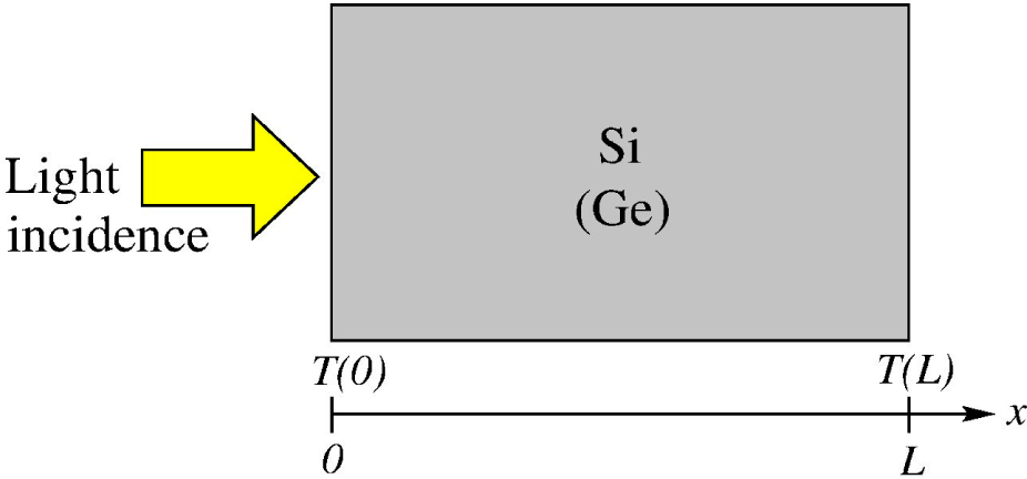
2.1. The System
2.2. Mathematical Model
2.3. The Reduced Model
2.4. Boundary Conditions
2.5. Solutions for n, p and T
2.6. Spectral Chebyshev Collocation Method
3. Results and Discussions
4. Conclusions
Acknowledgments
Author Contributions
Conflicts of Interest
Appendix
A. Thermodynamic Formalism
B. Optics
C. Dimensional Analysis
D. Constants
References
- Estrada-Wiese, D.; del Río, J.A.; de la Mora, M.B. Heat transfer in photonic mirrors. J. Mater. Sci. 2014, 25, 4348–4355. [Google Scholar]
- Boggi, S.; Razzitte, A.C.; Fano, W.G. Non-equilibrium thermodynamics and entropy production spectra: A tool for the characterization of ferromagnetic materials. J. Non-Equilib. Thermodyn. 2013, 38, 175–183. [Google Scholar]
- Vázquez, F.; del Río, J.A. Thermodynamic characterization of the diffusive transport to wave propagation transition in heat conducting thin films. J. Appl. Phys. 2012, 112, 123707. [Google Scholar]
- Figueroa, A.; Vázquez, F. Optimal performance and entropy generation transition from micro to nanoscaled thermoelectric layers. Int. J. Heat Mass Transf. 2014, 71, 724–731. [Google Scholar]
- Lucia, U. Stationary open systems: A brief review on contemporary theories on irreversibility. Physica A 2013, 392, 1051–1062. [Google Scholar]
- Goupil, C.; Seifert, W.; Zabrocki, K.; Müller, E.; Snyder, G.J. Thermodynamics of Thermoelectric Phenomena and Applications. Entropy 2011, 13, 1481–1517. [Google Scholar]
- Maldovan, M. Narrow Low-Frequency Spectrum and Heat Management by Thermocrystals. Phys. Rev. Lett. 2013, 110, 025902. [Google Scholar]
- Yilbas, B.S.; Al-Dweik, A.Y. Short-pulse heating and analytical solution to non-equilibrium heating process. Physica B 2013, 417, 28–32. [Google Scholar]
- Mansoor, S.B.; Yilbas, B.S. Laser short-pulse heating of silicon-aluminum thin films. Opt. Quant. Electron. 2011, 42, 601–618. [Google Scholar]
- Lewandowska, M.; Malinowski, L. An analytical solution of the hyperbolic heat conduction equation for the case of a finite medium symmetrically heated on both sides. Int. Commun. Heat Mass Transf. 2006, 33, 61–69. [Google Scholar]
- Barbagiovanni, E.G.; Loockwood, D.J.; Simpsom, P.J.; Goncharova, L.V. Quantum confinement in Si and Ge nanostructures: Theory and experiment. Appl. Phys. Rev. 2014, 1, 011302. [Google Scholar] [CrossRef]
- Zhao, S.; Yedlin, M.J. A new Iterative Chebyshev Spectral Method for Solving the Elliptic Equation . J. Comput. Phys. 1994, 113, 215–223. [Google Scholar]
- Peyret, R. Spectral Methods for Incompressible Viscous Flow, 5th ed.; Springer: New York, NY, USA, 2002. [Google Scholar]
- Joshi, A.A.; Majumdar, A. Transient ballistic and diffusive phonon heat transport in thin films. J. Appl. Phys. 1993, 74, 31–39. [Google Scholar]
- Wachutka, G.K. Rigorous thermodynamic treatment of heat generation and conduction in semiconductor device modeling. IEEE Trans. Comput. Aided Des. 1990, 9, 1141–1149. [Google Scholar]
- Muscato, O. The Onsager reciprocity principle as a check of consistency for semiconductor carrier transport models. Physica A 2001, 289, 422–458. [Google Scholar]
- Chen, W.H.; Wang, C.-C.; Hung, C.-I.; Yang, C.-C.; Juang, R.-C. Modeling and simulation for the design of thermal-concentrated solar thermoelectric generator. Energy 2014, 64, 287–297. [Google Scholar]
- Gupta, M.P.; Sayer, M.-H.; Mukhopadhyay, S.; Kumar, S. Ultrathin Thermoelectric Devices for On-Chip Peltier Cooling. IEEE Trans. Compon. Packag. Manuf. Technol. 2011, 1, 1395–1405. [Google Scholar]
- Singh, A.; Avasthi, D.V.; Singh, T.; Kumar, D. Design a Thermophotovoltaic System to Optimize Surface Radiative conductive heat flux. Int. J. Emerg. Trends Eng. Dev. 2014, 4, 216–222. [Google Scholar]
- Muscato, O.; di Stefano, V. Hydrodynamic simulation of a n+ − n − n+ Silicon nanowire. Contin. Mech. Thermodyn. 2014, 26, 197–205. [Google Scholar]
- Selberherr, S. Analysis and Simulation of Semiconductor Devices; Springer: Vienna, Austria, 1984. [Google Scholar]
- Jou, D.; Casas-Vázquez, J.; Lebon, G. Extended Irreversible Thermodynamics, 4th ed.; Springer: New York, NY, USA, Dordrecht, The Netherlands; Heidelberg, Germany; London, UK, 2001. [Google Scholar]
- Shockley, W.; Read, W.T. Statistics of the recombinations of holes and electrons. Phys. Rev. 1952, 87, 835–842. [Google Scholar]
- Sellito, A.; Cimmelli, V.; Jou, D. Thermoelectric effects and size dependency of the figure-of-merit in cylindrical nanowires. Int. J. Heat Mass Transf. 2013, 57, 109–116. [Google Scholar]
- De Groot, S.R.; Mazur, P. Non-Equilibrium Thermodynamics; Dover: New York, NY, USA, 1984. [Google Scholar]


| Material | |||||||
|---|---|---|---|---|---|---|---|
| Si | |||||||
| Ge |
| Material | ||||||||
|---|---|---|---|---|---|---|---|---|
| Si | 1.891 × 10⁻³ | 7.732 × 10⁻⁶ | 5.599 × 10⁻⁵ | 0 | 1.232 × 10⁷ | 1.959 × 10⁻³ | 1.155 × 10¹⁶ | 4.538 × 10¹⁵ |
| Ge | 4.662 × 10⁻² | 2.381 × 10⁻² | 7.999 × 10⁻² | 0 | 1.238 × 10⁷ | 1.599 × 10⁻¹ | 2.567 × 10¹⁹ | 1.634 × 10¹⁹ |
© 2015 by the authors; licensee MDPI, Basel, Switzerland This article is an open access article distributed under the terms and conditions of the Creative Commons Attribution license (http://creativecommons.org/licenses/by/4.0/).
Share and Cite
Nájera-Carpio, J.E.; Vázquez, F.; Figueroa, A. Modeling and Analysis of Entropy Generation in Light Heating of Nanoscaled Silicon and Germanium Thin Films. Entropy 2015, 17, 4786-4808. https://0-doi-org.brum.beds.ac.uk/10.3390/e17074786
Nájera-Carpio JE, Vázquez F, Figueroa A. Modeling and Analysis of Entropy Generation in Light Heating of Nanoscaled Silicon and Germanium Thin Films. Entropy. 2015; 17(7):4786-4808. https://0-doi-org.brum.beds.ac.uk/10.3390/e17074786
Chicago/Turabian StyleNájera-Carpio, José Ernesto, Federico Vázquez, and Aldo Figueroa. 2015. "Modeling and Analysis of Entropy Generation in Light Heating of Nanoscaled Silicon and Germanium Thin Films" Entropy 17, no. 7: 4786-4808. https://0-doi-org.brum.beds.ac.uk/10.3390/e17074786