
A New Chaotic System with Positive Topological Entropy

Abstract
:1. Introduction
- (a)
- The system has a simple algebraic structure including one constant term, two linear terms and two nonlinear terms.
- (b)
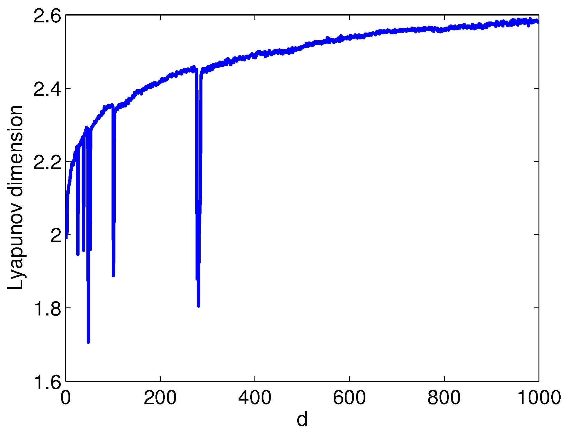
- With some typical parameters, the Lyapunov dimension of the considered system is greater than other known 3D chaotic systems
- (c)
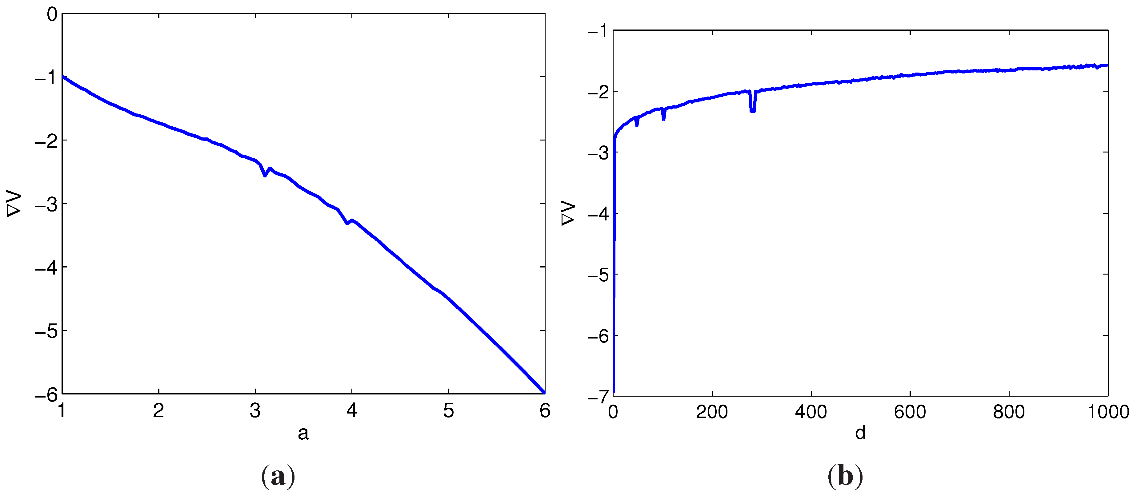
- The divergence of flow of the proposed system is not a constant but is always less than zero, while it’s a negative constant for other known 3D chaotic systems. The bigger the divergence is, the more scattered the phase trajectory is.
- (d)
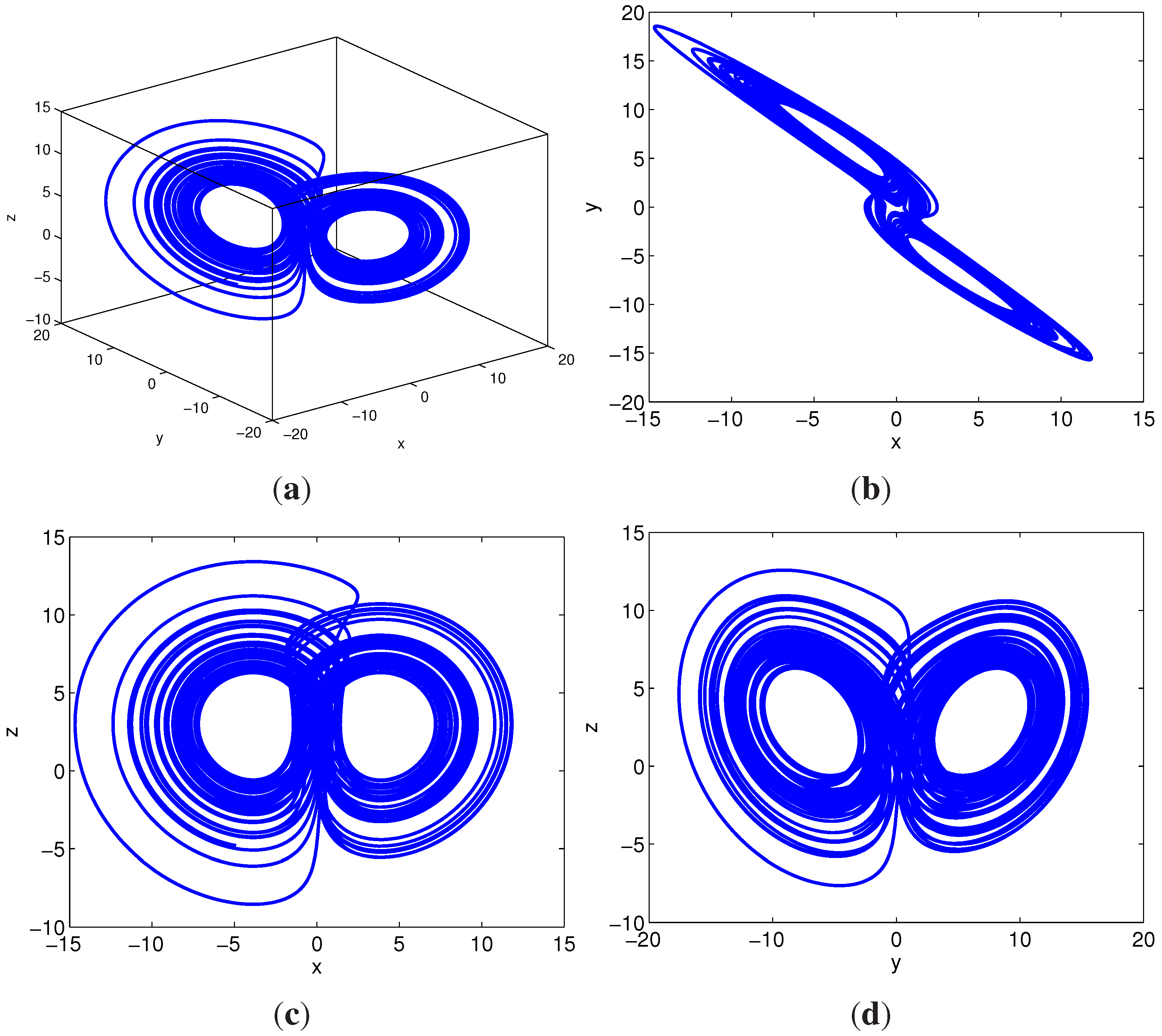
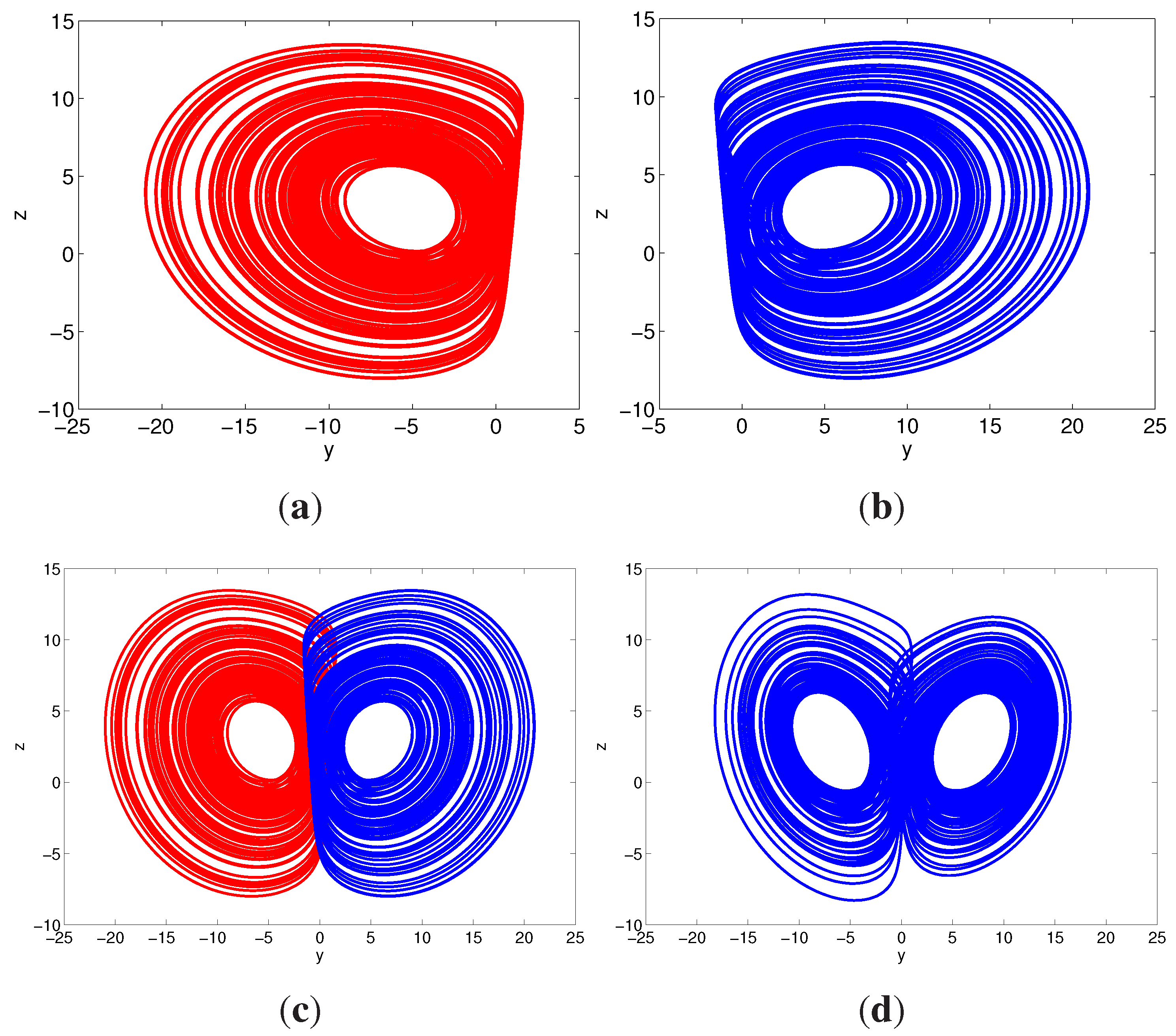
- The proposed chaotic attractor has a compound structure which can be demonstrated using a half-image operation to obtain the left or the right half-image attractors.
- (e)
- The system exhibits chaotic behavior over a large range of parameters.
2. The New Chaotic System and Its Basic Properties
2.1. System Description
2.2. Non-generalized Lorenz System
2.3. Equilibria
3. Observation and Analysis of the New System
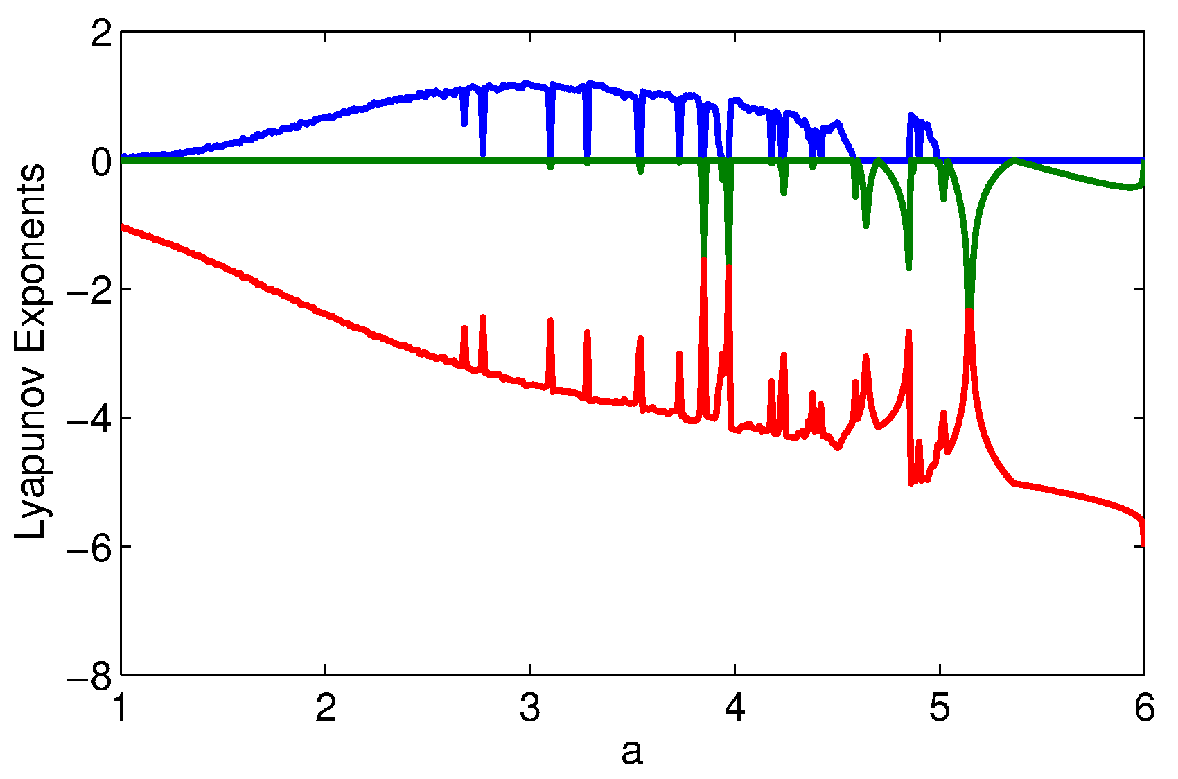
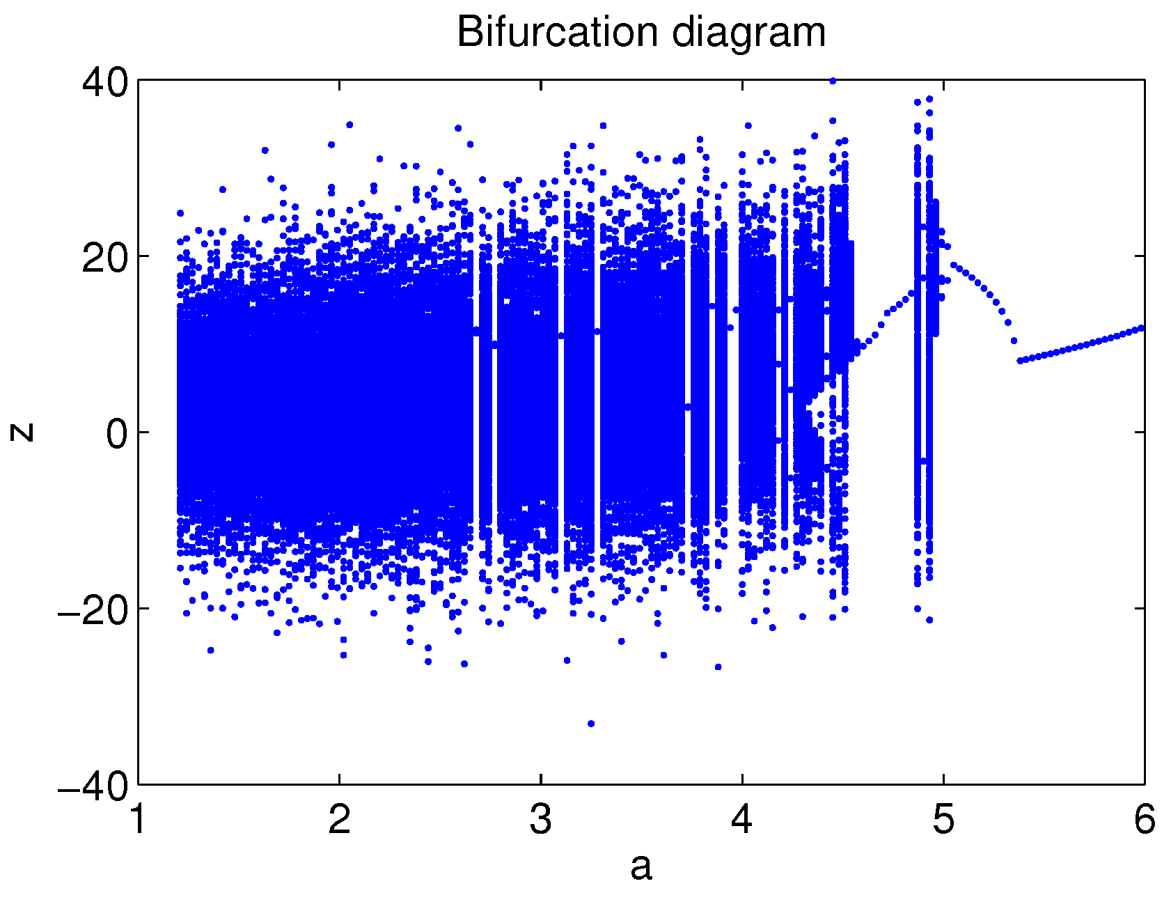
3.1. Fixing and Varying a
- (1)
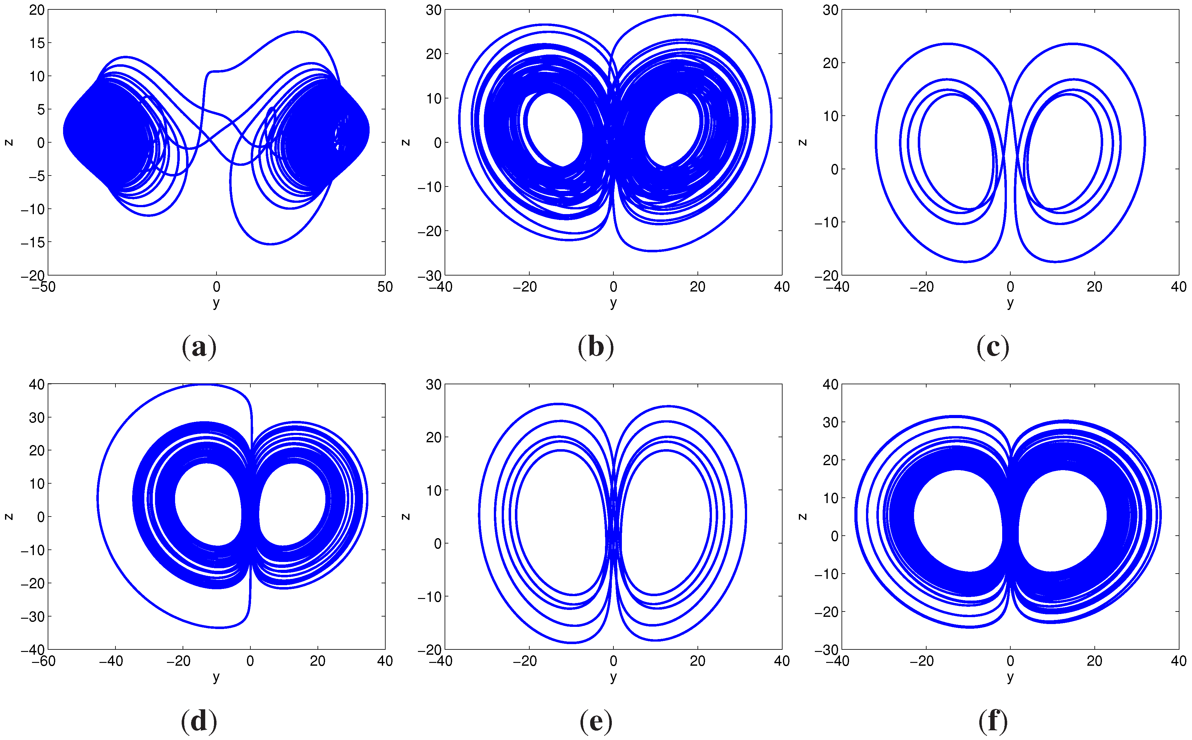
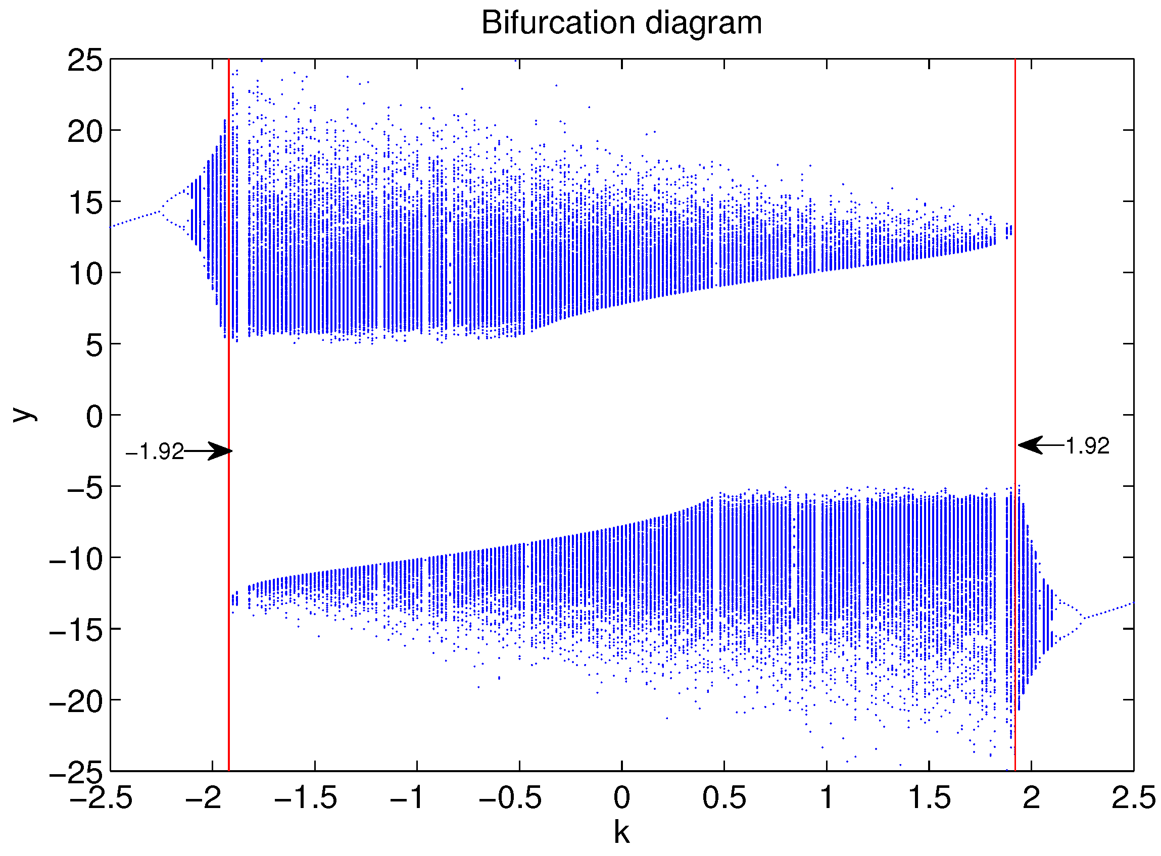
- When , we can obtain , and both and are less than 0, and the trajectories started from different initial conditions approach a closed orbit surrounding two equilibria. For example, the periodic orbits for and are depicted in Figure 3c,e,h, respectively. When , there is a vertical white region, that’s because the system (3) has a 2-periodic orbit within this range. The low density of trajectories leads to the low density of the points in the bifurcation diagram.
- (2)
- When a belongs to , and , and strange chaotic attractors will appear. When and , some double-scroll chaotic attractors are shown in Figure 3a,b,d,f,g, respectively.


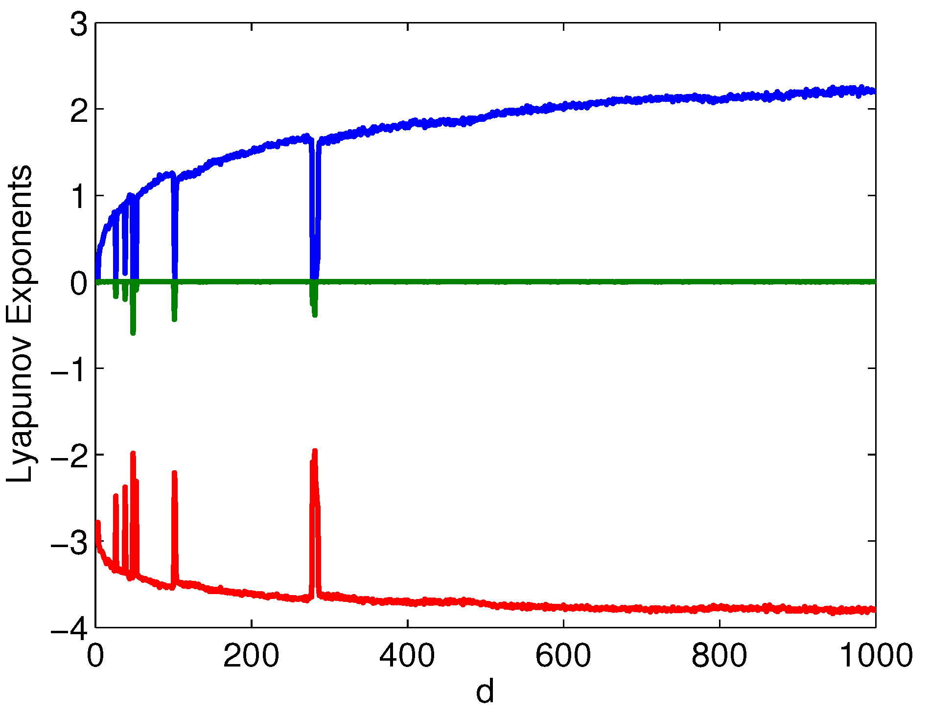
3.2. Fixing and Varying d


3.3. A Dissipative System

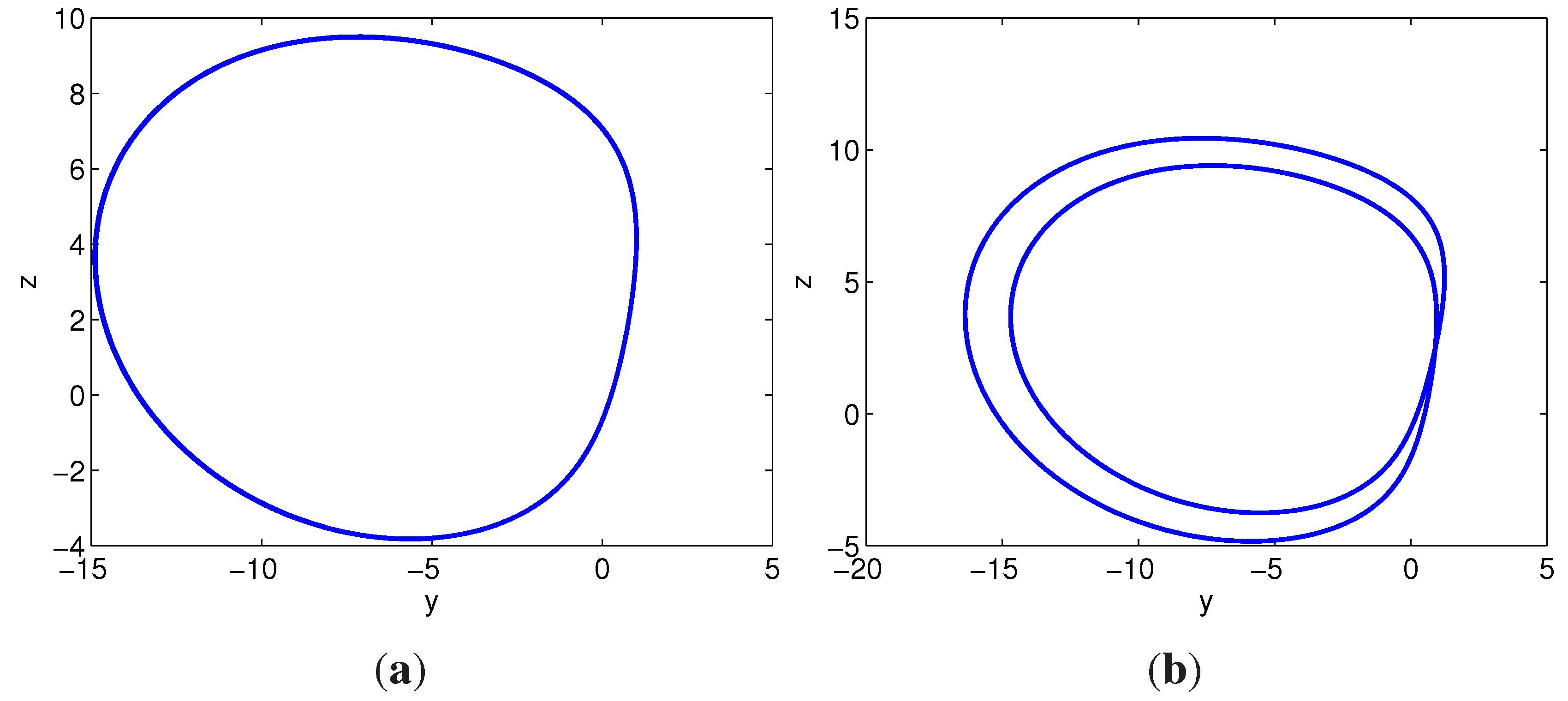
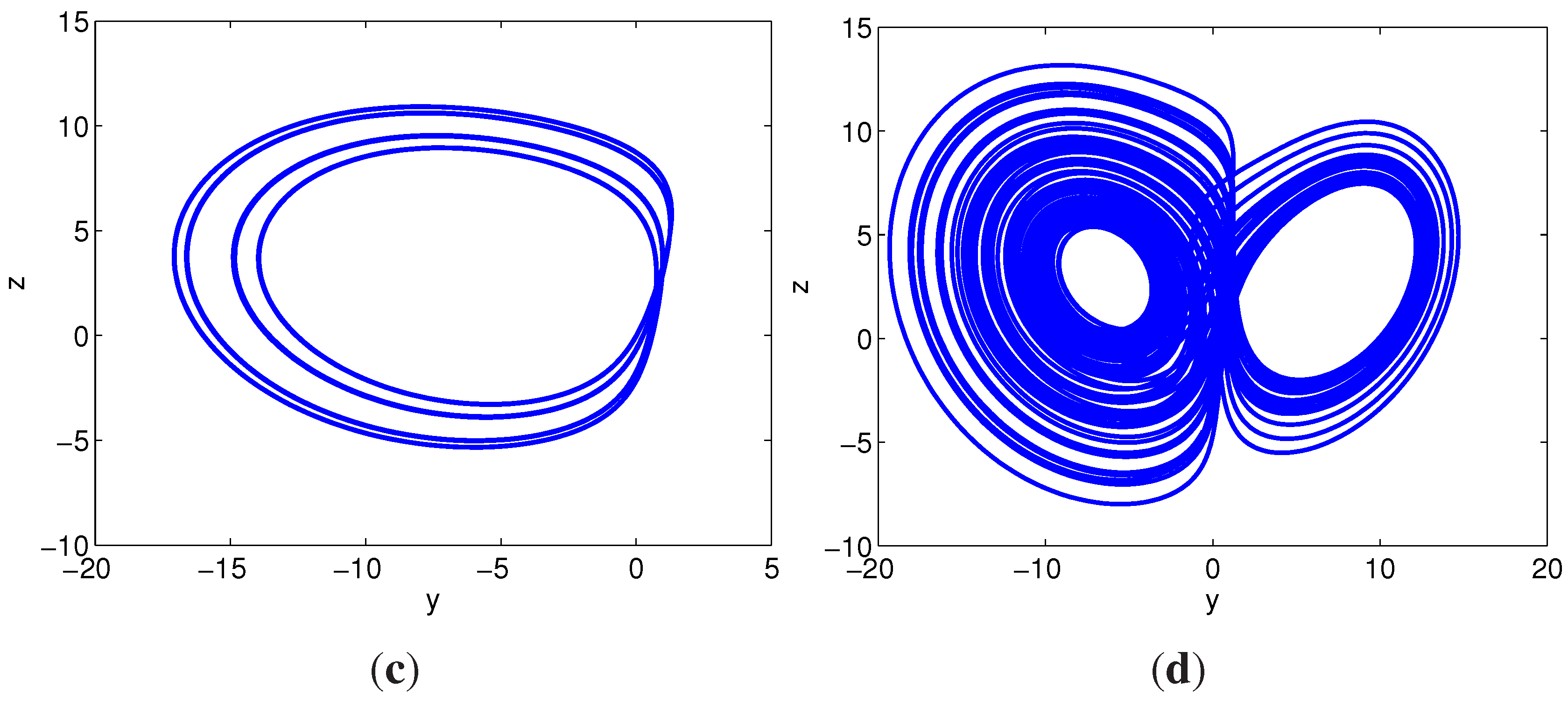
3.4. Compound Structures

- (1)
- When , the system (14) has limit cycles. For example, Figure 11a shows a limit cycle at .
- (2)
- When , there are period-doubling bifurcations. For example, Figure 11b,c show such period-doubling bifurcations at and , respectively.
- (3)
- When , the system (14) becomes a left (or a right) half-image attractor as shown in Figure 9a,b.
- (4)
- When , the system demonstrates partial attractors, which are bounded. For example, Figure 11d shows a partially-right, dominantly-left, attractor at .
- (5)
- For , the system exhibits a complete attractor. For example, Figure 5 shows the complete attractor at .


4. Topological Horseshoe Analysis for the New Chaotic System
4.1. Review of a Topological Horseshoe Theory
- (i)
- ;
- (ii)
- σ is continuous;
- (iii)
- σ has countable many periodic orbits;
- (iv)
- σ has uncountable many aperiodic orbits;
- (v)
- σ has a dense orbit.
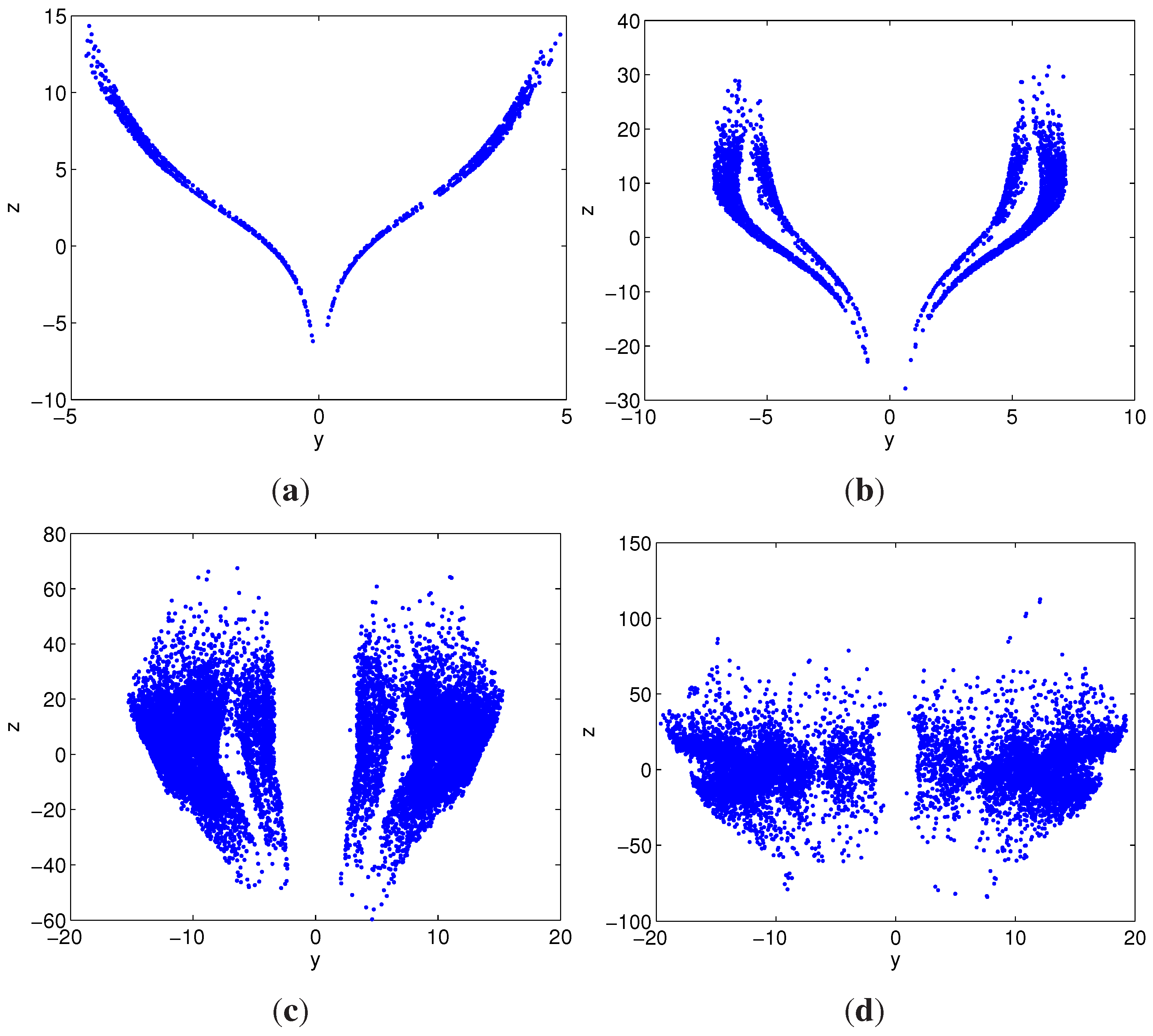
4.2. Horseshoe in the Poincaré Map for the Proposed System


5. Conclusions
Acknowledgments
Author Contributions
Conflicts of Interest
References
- Wang, S.; Kuang, J.; Li, J.; Luo, Y.; Lu, H.; Hu, G. Chaos-Based Secure Communications in a Large Community. Phys. Rev. E 2002, 66, 065202. [Google Scholar] [CrossRef]
- Zhang, W.; Wong, K.W.; Yu, H.; Zhu, Z.L. An Image Encryption Scheme Using Reverse 2-Dimensional Chaotic Map and Dependent Diffusion. Commun. Nonlinear Sci. Numer. Simul. 2013, 18, 147–148. [Google Scholar] [CrossRef]
- Yalcin, M.; Özoǧuz, S.; Suykens, J. N-scroll Chaos Generators: A Simple Circuit Model. Electron. Lett. 2001, 37, 645–664. [Google Scholar] [CrossRef]
- Buscarino, A.; Fortuna, L.; Frasca, M.; Gambuzza, L.V. A Chaotic Circuit Based on Hewlett-Packard Memristor. Chaos 2012, 22, 023136. [Google Scholar] [CrossRef] [PubMed]
- Wang, J.; Tang, W.; Zhang, J. Approximate Synchronization of Two Non-linear Systems via Impulsive Control. Proc. Inst. Mech. Eng. Part I 2012, 226, 338–347. [Google Scholar] [CrossRef]
- Suykens, J.; Yalçın, M.; Vandewalle, J. Chaotic Systems Synchronization. In Chaos Control; Springer: Berlin, Germany, 2003; Volume 292, pp. 117–135. [Google Scholar]
- Wu, X.; Lu, J.A.; Chi, K.T.; Wang, J.; Liu, J. Impulsive Control and Synchronization of the Lorenz Systems Family. Chaos Solitons Fractals 2007, 31, 631–638. [Google Scholar] [CrossRef]
- Lorenz, E.N. Deterministic Nonperiodic Flow. J. Atmos. Sci. 1963, 20, 130–141. [Google Scholar] [CrossRef]
- Rössler, O.E. An Equation for Continuous Chaos. Phys. Lett. A 1976, 57, 397–398. [Google Scholar] [CrossRef]
- Chua, L.O.; Komuro, M.; Matsumoto, T. The Double Scroll Family. IEEE Trans. Circuits Syst. 1986, 33, 1073–1118. [Google Scholar] [CrossRef]
- Sprott, J. Some Simple Chaotic Flows. Phys. Rev. E 1994, 50, R647. [Google Scholar] [CrossRef]
- Chen, G.; Ueta, T. Yet Another Chaotic Attractor. Int. J. Bifurc. Chaos 1999, 9, 1465–1466. [Google Scholar] [CrossRef]
- May, R.M. Simple Mathematical Models with very Complicated Dynamics. Nature 1976, 261, 459–467. [Google Scholar] [CrossRef] [PubMed]
- Hénon, M. A Two-Dimensional Mapping with a Strange Attractor. Commun. Math. Phys. 1976, 50, 69–77. [Google Scholar] [CrossRef]
- Lozi, R. Un Attracteur Étrange (?) du Type Attracteur de Hénon. Le J. Phys. Colloq. 1978, 39, C5-9–C5-10. [Google Scholar]
- Lü, J.; Chen, G. A New Chaotic Attractor Coined. Int. J. Bifurc. Chaos 2002, 12, 659–661. [Google Scholar] [CrossRef]
- Smale, S. Differentiable Dynamical Systems. Bull. Am. Math. Soc. 1967, 73, 747–817. [Google Scholar] [CrossRef]
- Li, Q.; Yang, X.S. A Simple Method for Finding Topological Horseshoes. Int. J. Bifurc. Chaos 2010, 20, 467–478. [Google Scholar] [CrossRef]
- Li, Q.; Zhang, L.; Yang, F. An Algorithm to Automatically Detect the Smale Horseshoes. Discret. Dyn. Nat. Soc. 2012, 31, 726–737. [Google Scholar] [CrossRef]
- Zgliczynski, P. Computer Assisted Proof of Chaos in the Rössler Equations and in the Hénon Map. Nonlinearity 1997, 10, 243–252. [Google Scholar] [CrossRef]
- Mischaikow, K.; Mrozek, M. Chaos in the Lorenz Equations: A Computer-Assisted Proof. Bull. Am. Math. Soc. 1995, 32, 66–72. [Google Scholar] [CrossRef]
- Mischaikow, K.; Mrozek, M. Chaos in the Lorenz Equations: A Computer-Assisted Proof. Part II: Details. Math. Comput. Am. Math. Soc. 1997, 33, 66–72. [Google Scholar] [CrossRef]
- Li, Q.; Shu, C.; Ping, Z. Horseshoe and Entropy in a Fractional-Order Unified System. Chin. Phys. B 2011, 20, 010502. [Google Scholar] [CrossRef]
- Li, Q.; Yang, X.S. Chaotic Dynamics in a Class of Three Dimensional Glass Networks. Chaos Interdiscip. J. Nonlinear Sci. 2006, 16, 033101. [Google Scholar] [CrossRef] [PubMed]
- Huan, S.; Li, Q.; Yang, X.S. Horseshoes in a Chaotic System with only One Stable Equilibrium. Int. J. Bifurc. Chaos 2013, 01, 23. [Google Scholar] [CrossRef]
- Čelikovský, S.; Chen, G. On a Generalized Lorenz Canonical Form of Chaotic Systems. Int. J. Bifurc. Chaos 2002, 12, 1789–1812. [Google Scholar] [CrossRef]
- Čelikovský, S.; Chen, G. On the Generalized Lorenz Canonical Form. Chaos Solitons Fractals 2005, 26, 1271–1276. [Google Scholar] [CrossRef]
- Yang, Q.; Chen, G.; Zhou, T. A Unified Lorenz-type System and Its Canonical Form. Int. J. Bifurc. Chaos 2006, 16, 2855–2871. [Google Scholar] [CrossRef]
- Yang, Q.; Zhang, K.; Chen, G. A Modified Generalized Lorenz-type System and Its Canonical Form. Int. J. Bifurc. Chaos 2009, 19, 1931–1949. [Google Scholar] [CrossRef]
- Šil’nikov, L. A Contribution to the Problem of the Structure of an Extended Neighborhood of a Rough Equilibrium State of Saddle-Focus Type. Math. USSR SB 1970, 10, 91–102. [Google Scholar] [CrossRef]
- Shilnikov, L.P.; Shilnikov, A.L.; Turaev, D.V.; Chua, L.O. Methods of Qualitative Theory in Nonlinear Dynamics; World Scientific: Singapore, Singapore, 2001; pp. 393–957. [Google Scholar]
- Sprott, J. Maximally Complex Simple Attractors. Chaos 2007, 17, 033124. [Google Scholar] [CrossRef] [PubMed]
- Lü, J.; Chen, G.; Zhang, S. The Compound Structure of a New Chaotic Attractor. Chaos Solitons Fractals 2002, 14, 669–672. [Google Scholar] [CrossRef]
- Galias, Z. Positive Topological Entropy of Chua’s Circuit: A Computer Assisted Proof. Int. J. Bifurc. Chaos 1997, 7, 331–349. [Google Scholar] [CrossRef]
- Galias, Z.; Zgliczyński, P. Computer Assisted Proof of Chaos in the Lorenz Equations. Physica D 1998, 115, 165–188. [Google Scholar] [CrossRef]
- Wiggins, S.; Golubitsky, M. Introduction to Applied Nonlinear Dynamical Systems and Chaos; Springer: Berlin, Germany, 1990; pp. 555–584. [Google Scholar]
- Robinson, C. Dynamical Systems: Stability, Symbolic Dynamics, and Chaos; CRC Press: Boca Raton, FL, USA, 1995. [Google Scholar]
- Yang, X.S.; Li, Q. A Computer-Assisted Proof of Chaos in Josephson Junctions. Chaos Solitons Fractals 2006, 27, 25–30. [Google Scholar] [CrossRef]
- Yang, X.S.; Tang, Y. Horseshoes in Piecewise Continuous Maps. Chaos Solitons Fractals 2004, 19, 841–845. [Google Scholar] [CrossRef]
© 2015 by the authors; licensee MDPI, Basel, Switzerland. This article is an open access article distributed under the terms and conditions of the Creative Commons Attribution license (http://creativecommons.org/licenses/by/4.0/).
Share and Cite
Wang, Z.; Ma, J.; Chen, Z.; Zhang, Q. A New Chaotic System with Positive Topological Entropy. Entropy 2015, 17, 5561-5579. https://0-doi-org.brum.beds.ac.uk/10.3390/e17085561
Wang Z, Ma J, Chen Z, Zhang Q. A New Chaotic System with Positive Topological Entropy. Entropy. 2015; 17(8):5561-5579. https://0-doi-org.brum.beds.ac.uk/10.3390/e17085561
Chicago/Turabian StyleWang, Zhonglin, Jian Ma, Zengqiang Chen, and Qing Zhang. 2015. "A New Chaotic System with Positive Topological Entropy" Entropy 17, no. 8: 5561-5579. https://0-doi-org.brum.beds.ac.uk/10.3390/e17085561