
Combined Power Quality Disturbances Recognition Using Wavelet Packet Entropies and S-Transform

Abstract
:1. Introduction
2. Wavelet Packet Entropies and Modified Incomplete S-Transform
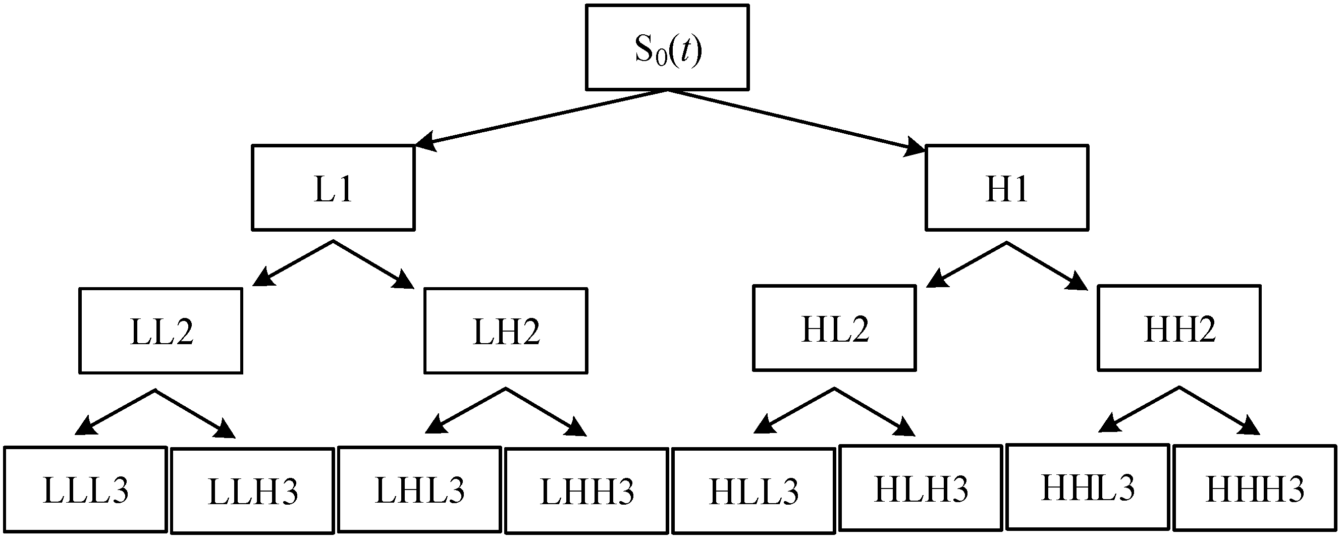
2.1. Wavelet Packet Decomposition

2.2. Shannon Entropy and Wavelet Packet Energy Entropy
2.3. Tsallis Entropy and Wavelet Packet Tsallis Entropy
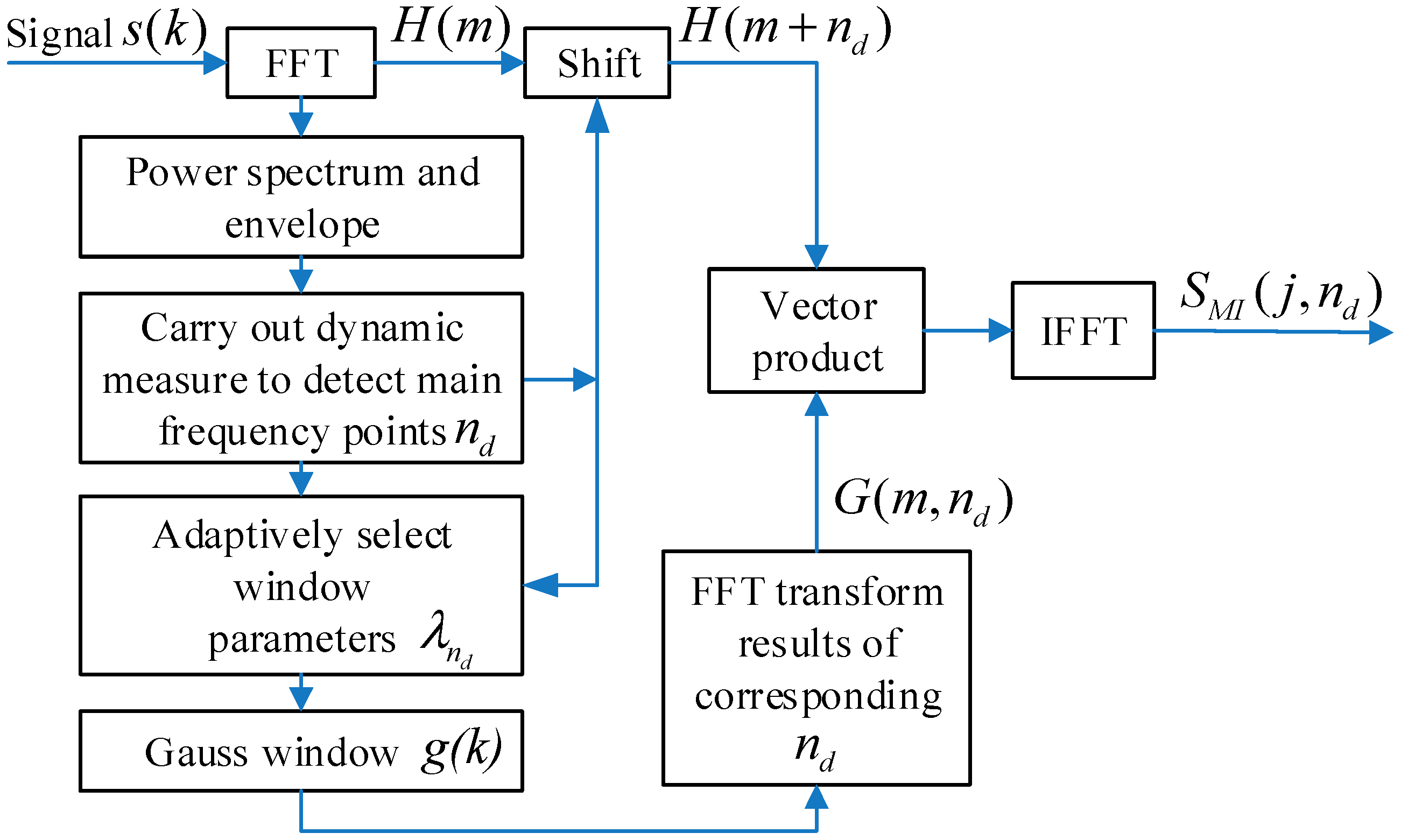
2.4. Modified Incomplete S-Transform

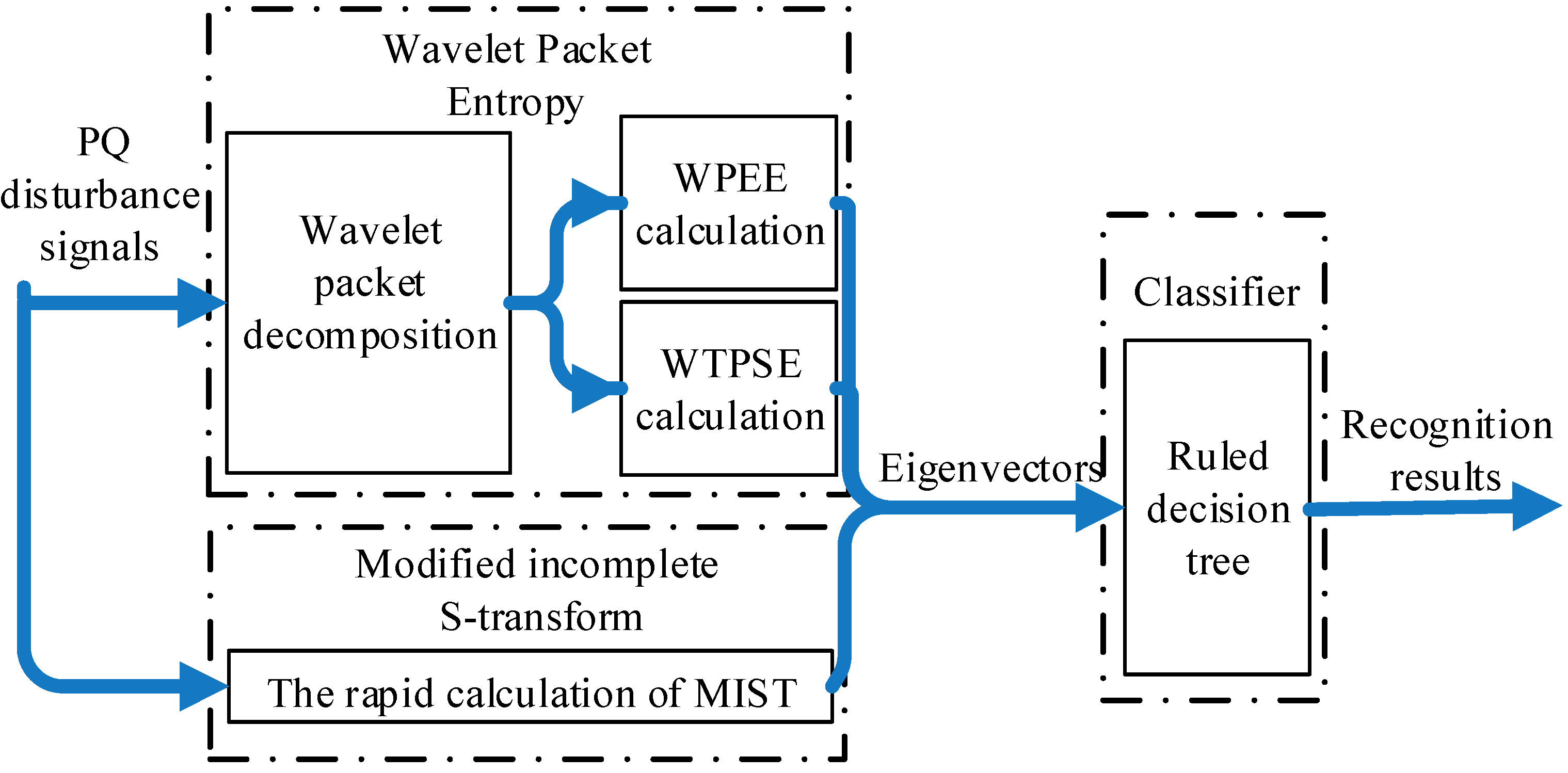
3. Recognition Plan

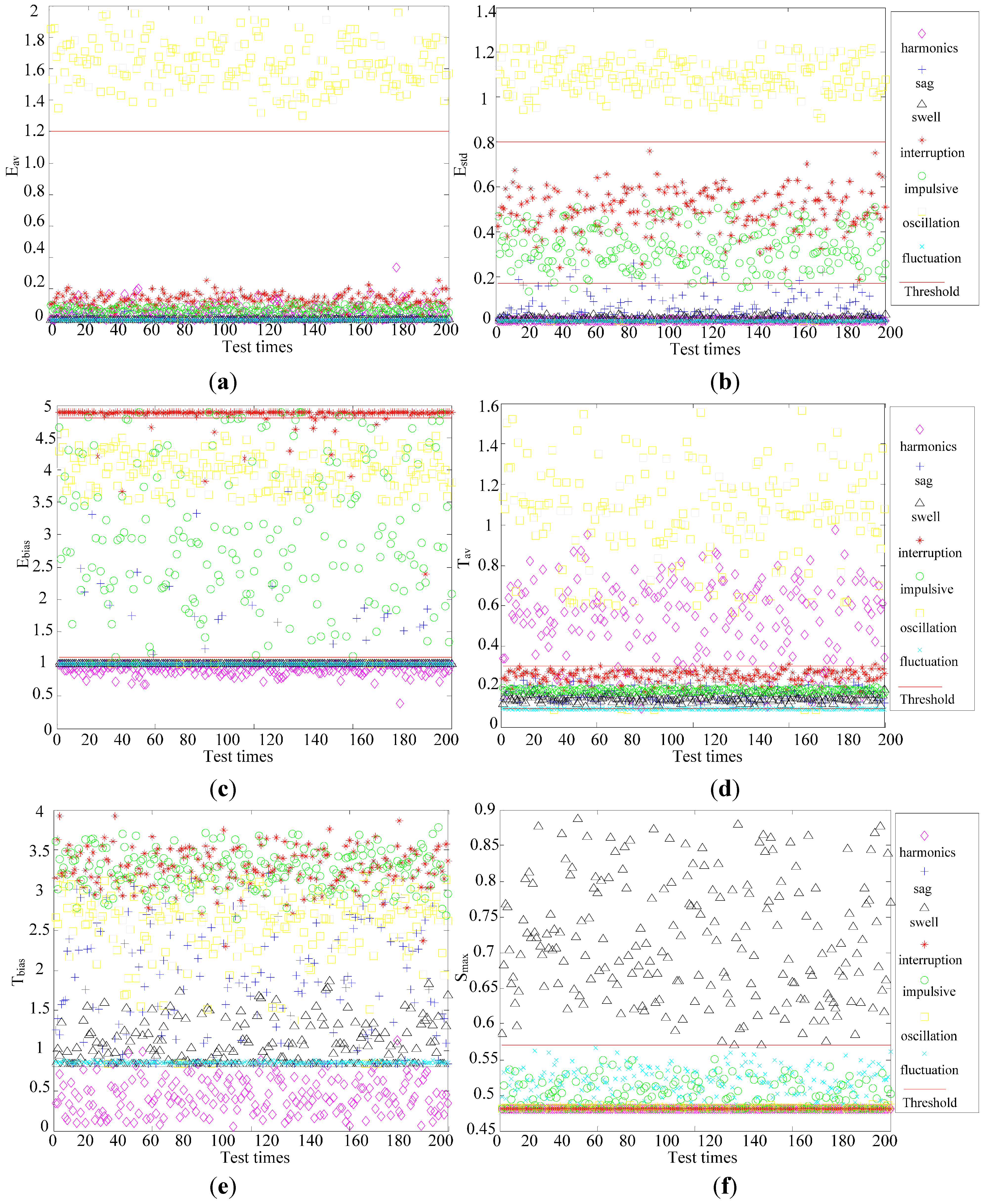
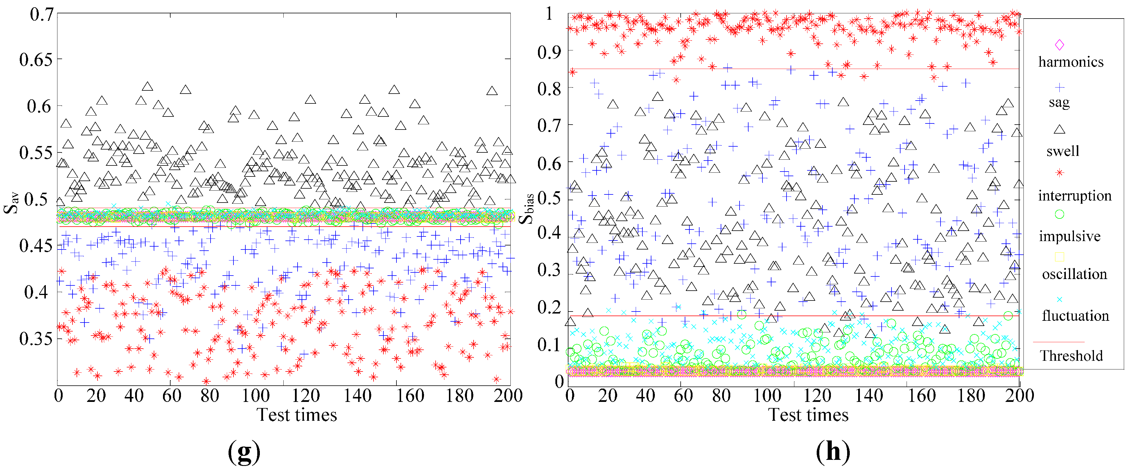
3.1. Feature Extraction

| No | Method | Name | Description | Threshold | Function |
|---|---|---|---|---|---|
| 1 | WPEE | Eav | Mean value | 1.2 | Oscillation assistant judgment |
| 2 | Estd | Standard deviation | 0.17, 0.8 | Impulsive/oscillation assistant judgment | |
| 3 | Ebias | Bias | 1.1, 4.8 | Interruption/impulsive assistant judgment | |
| 4 | WPTSE | Eav | Mean value | 0.091, 0.35 | Oscillation/impulsive assistant judgment |
| 5 | Ebias | Bias | 0.8 | Harmonic assistant judgment | |
| 6 | MIST | Nf | Number of main frequency points | - | Oscillation/harmonic initial judgment |
| 7 | Nh | Whether it contains high frequency | 0, 1 | Oscillation initial judgment | |
| 8 | N1 | Whether it contains Harmonic | 0, 1 | Harmonic initial judgment | |
| 9 | Sav | Average amplitude of the fundamental components | 0.475, 0.495 | Swell/sag/interruption initial judgment | |
| 10 | Sbias | Bias of the fundamental component | 0.19, 0.85 | Swell/sag/interruption initial judgment | |
| 11 | Smax | Maximum of the fundamental component | 0.4807, 0.57 | Swell/sag/interruption assistant judgment | |
| 12 | S_1 | Amplitude fluctuation of fundamental components | 0, 1 | Fluctuation assistant judgment | |
| 13 | S_2 | The symmetry of main frequency points | 0, 1 | Fluctuation assistant judgment |
| Disturbances | Eav | Estd | Ebias | Tav | Tbias | Nf | Nh | N1 | Sav | Sbias | Smax | S_1 | S_2 |
|---|---|---|---|---|---|---|---|---|---|---|---|---|---|
| Normal (R0) | 0.0006 | 0.0009 | 0.9991 | 0.0882 | 0.8392 | 1 | 0 | 0 | 0.4806 | 0.0387 | 0.4806 | 0 | 0 |
| Swell (R1) | 0.0016 | 0.0041 | 0.9991 | 0.1377 | 0.8398 | 1 | 0 | 0 | 0.5576 | 0.4072 | 0.7036 | 0 | 0 |
| Sag (R2) | 0.0022 | 0.0065 | 0.9991 | 0.1374 | 0.8824 | 1 | 0 | 0 | 0.4392 | 0.2841 | 0.4806 | 0 | 0 |
| Interruption (R3) | 0.0986 | 0.4007 | 4.8617 | 0.2519 | 3.5527 | 1 | 0 | 0 | 0.3537 | 0.9615 | 0.4806 | 0 | 1 |
| Impulsive (R4) | 0.0686 | 0.3500 | 3.4339 | 0.1809 | 3.4694 | 1 | 0 | 0 | 0.4767 | 0.1130 | 0.4806 | 0 | 0 |
| Oscillation (R5) | 1.5776 | 1.0600 | 3.7398 | 0.6735 | 2.1716 | 2 | 1 | 0 | 0.4811 | 0.0387 | 0.4830 | 0 | 0 |
| Harmonics (R6) | 0.0409 | 0.0027 | 0.9322 | 0.5730 | 0.1735 | 2 | 0 | 1 | 0.4806 | 0.0387 | 0.4806 | 0 | 0 |
| Fluctuation (R7) | 0.0007 | 0.0010 | 0.9991 | 0.0891 | 0.8423 | 1 | 0 | 0 | 0.4808 | 0.1402 | 0.5314 | 1 | 1 |


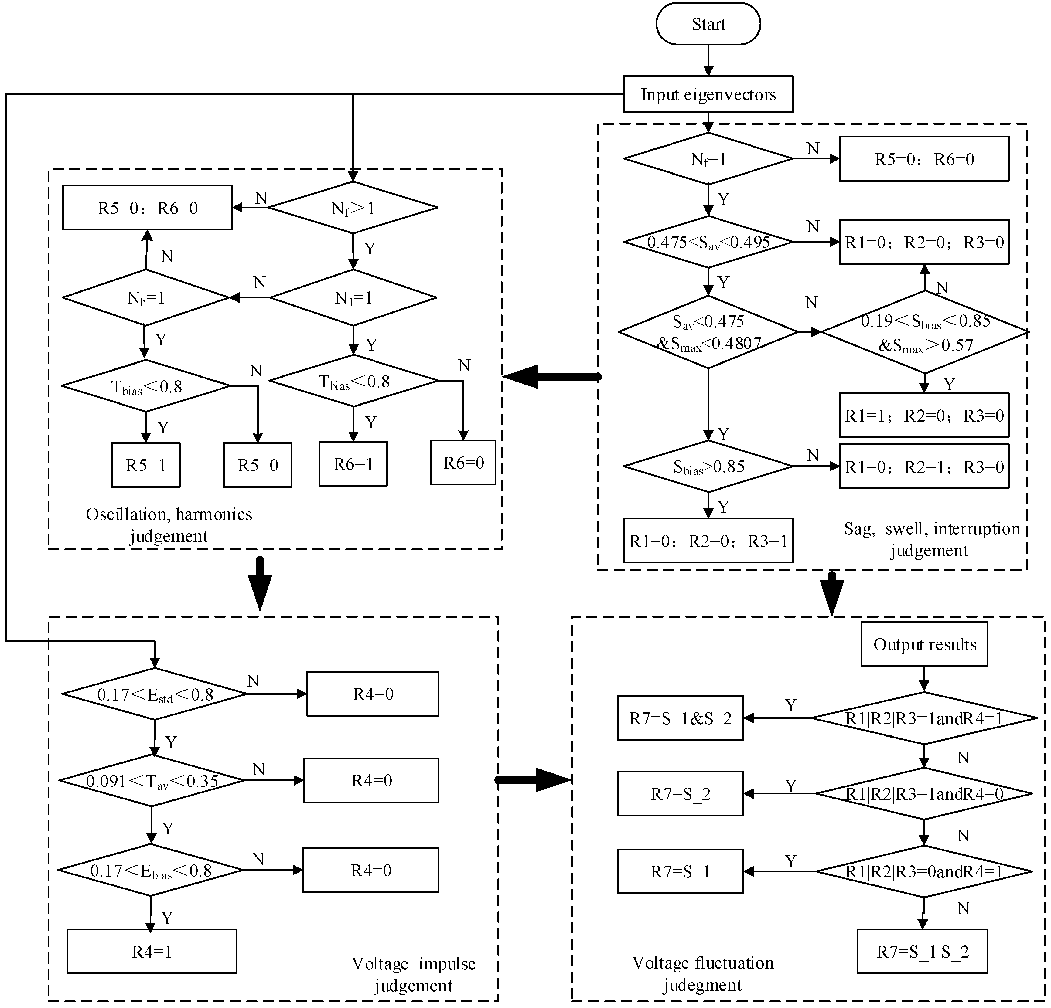
3.2. Ruled Decision Tree
| Rule | Description |
|---|---|
| Rule1 | if Sav > 0.495 & 0.19 < Sbias < 0.85 & Smax > 0.57 then R1 = 1 |
| Rule2 | if Sav < 0.475 & 0.19 < Sbias < 0.85 & Smax < 0.4807 then R2 = 1 |
| Rule 3 | if Sav < 0.475 & Sbias > 0.85 & Smax < 0.4807 then R3 = 1 |
| Rule 4 | if 0.17 < Estd < 0.8 & 0.091 < Tav < 0.35 & 1.1 < Ebias < 4.8 & Nh = 0 & N1 = 0 then R4 = 1 |
| Rule 5 | if Nf > 1& Nh = 1& Eav > 1.2 & Estd > 0.8 then R5 = 1 |
| Rule 6 | if Nf > 1& N1 = 1 & Tbias < 0.8 then R6 = 1 |
| Rule 7 | if R1|R2|R3 = 1 & R4 = 1 then R7 = S_1 & S_2 else if R1|R2|R3 = 1 & R4 = 0 then R7 = S_2 else if R1|R2|R3 = 0 & R4 = 1 then R7 = S_1 else R1|R2|R3 = 0 & R4 = 0 then R7 = S_1| S_2 |
3.3. Recognition Flow

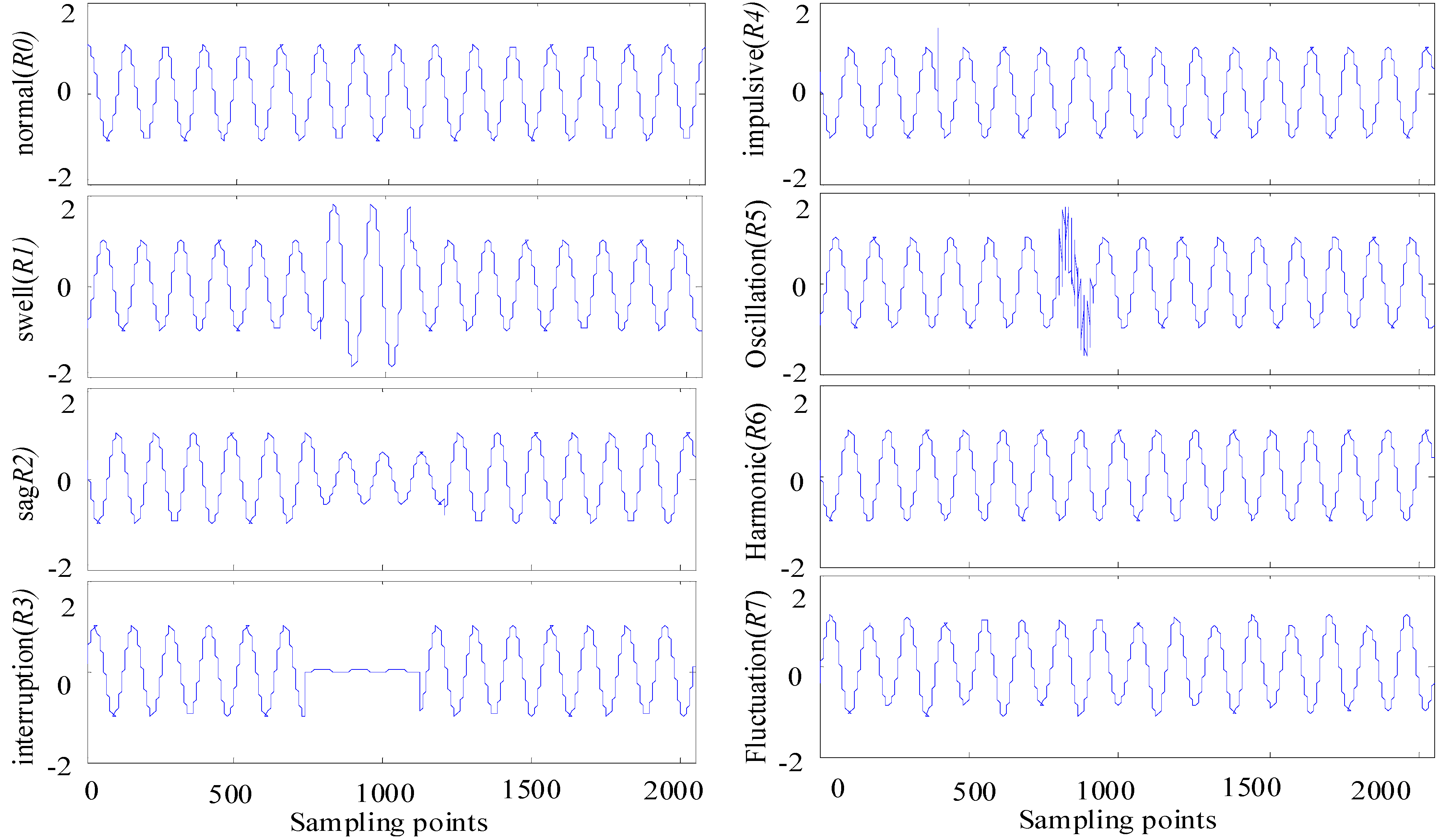
4. Experimental Results
| Disturbance Type | Recognition Results | Number of Right Samples | Accuracy/% | Time/s | ||||||
|---|---|---|---|---|---|---|---|---|---|---|
| R1 | R2 | R3 | R4 | R5 | R6 | R7 | ||||
| swell | 191 | 0 | 0 | 0 | 0 | 0 | 0 | 191 | 95.5 | 0.014 |
| sag | 0 | 189 | 10 | 0 | 0 | 0 | 0 | 189 | 94.5 | 0.018 |
| interruption | 0 | 5 | 195 | 0 | 0 | 0 | 0 | 195 | 97.5 | 0.014 |
| impulsive | 0 | 0 | 0 | 185 | 0 | 0 | 0 | 185 | 92.5 | 0.014 |
| oscillation | 0 | 0 | 0 | 0 | 194 | 0 | 0 | 194 | 97 | 0.011 |
| harmonics | 0 | 0 | 0 | 0 | 0 | 199 | 0 | 199 | 99.5 | 0.011 |
| fluctuation | 0 | 0 | 0 | 0 | 0 | 0 | 200 | 200 | 100 | 0.013 |
| Disturbance Type | Recognition Results | Number of Right Samples | Accuracy/% | Time/s | ||||||
|---|---|---|---|---|---|---|---|---|---|---|
| R1 | R2 | R3 | R4 | R5 | R6 | R7 | ||||
| R1 + R6 | 193 | 0 | 0 | 0 | 0 | 199 | 0 | 193 | 96.5 | 0.017 |
| R2 + R5 | 0 | 194 | 0 | 0 | 196 | 0 | 0 | 194 | 97 | 0.017 |
| R2 + R6 | 0 | 195 | 0 | 0 | 0 | 199 | 0 | 195 | 97.5 | 0.015 |
| R2 + R7 | 0 | 188 | 0 | 0 | 0 | 0 | 197 | 188 | 94 | 0.013 |
| R3 + R6 | 0 | 0 | 195 | 0 | 0 | 195 | 0 | 195 | 97.5 | 0.016 |
| R5 + R6 | 0 | 0 | 0 | 0 | 195 | 196 | 0 | 195 | 97.5 | 0.011 |
| R5 + R7 | 0 | 0 | 0 | 0 | 194 | 0 | 200 | 194 | 97 | 0.013 |
| R6 + R7 | 0 | 0 | 0 | 0 | 0 | 200 | 200 | 200 | 100 | 0.013 |
| R2 + R5 + R6 | 0 | 192 | 0 | 0 | 198 | 199 | 0 | 192 | 96 | 0.013 |
| R2 + R5 + R7 | 0 | 186 | 0 | 0 | 193 | 0 | 191 | 186 | 93 | 0.014 |
| R2 + R6 + R7 | 0 | 182 | 0 | 0 | 0 | 199 | 194 | 182 | 91 | 0.016 |
| R3 + R5 + R6 | 0 | 0 | 188 | 0 | 195 | 180 | 0 | 180 | 90 | 0.018 |
| R5 + R6 + R7 | 0 | 0 | 0 | 0 | 195 | 197 | 200 | 195 | 97.5 | 0.020 |
| R1+R4+R6+R7 | 181 | 0 | 0 | 194 | 0 | 198 | 196 | 181 | 90.5 | 0.020 |
- (1)
- Sample recognition accuracy. This index considers the overall recognition accuracy of the sample. It is a traditional pattern recognition evaluation method. The calculation formula is as follows.
- (2)
- Label error (leak) rate. This index considers the number of recognition error and leakage in recognition results of all samples. It reflects the stability of the proposed recognition method for single disturbance in the case of different combined disturbances. The calculation formula is as follows.
| Disturbance type | R1 | R2 | R3 | R4 | R5 | R6 | R7 |
|---|---|---|---|---|---|---|---|
| Total sample number | 14 × 200 = 2800 | ||||||
| Recognition error and leakage number | 26 | 31 | 17 | 6 | 27 | 37 | 7 |
| Recognition error and leakage rate/% | 0.928 | 1.107 | 0.607 | 0.214 | 0.964 | 1.321 | 0.250 |

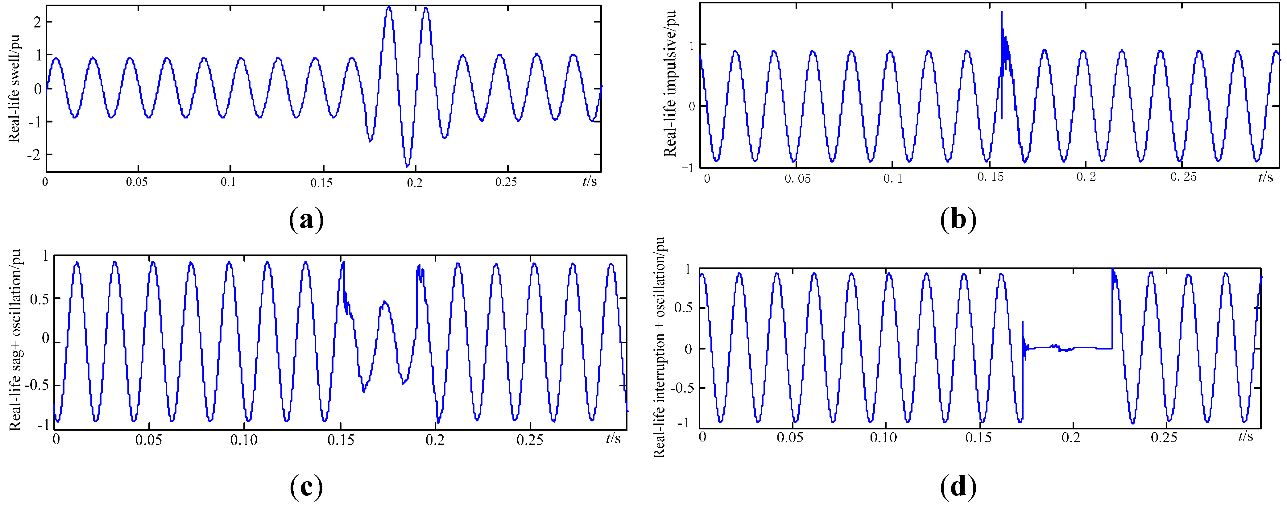
| Disturbances | R1 | R2 | R3 | R4 | R5 | R6 | R7 |
|---|---|---|---|---|---|---|---|
| Swell | 1 | 0 | 0 | 0 | 0 | 0 | 0 |
| Impulsive | 0 | 0 | 0 | 1 | 0 | 0 | 0 |
| Sag + Oscillation | 0 | 1 | 0 | 0 | 1 | 0 | 0 |
| Interruption + Oscillation | 0 | 0 | 1 | 0 | 1 | 0 | 0 |
| Method | Accuracy/% | |
|---|---|---|
| Single | Combined | |
| Improved incomplete S-transform with decision tree | 81.86 | 88.93 |
| Wavelet transform with neural network | 94.42 | 83.33 |
| EEMD and MIST with automatic classification | 97.70 | 88.70 |
| Wavelet Packet Entropies and MIST with decision tree (proposed) | 96.64 | 95.36 |
5. Conclusions
Acknowledgments
Author Contributions
Conflicts of Interest
References
- Valtierra-Rodriguez, M.; de Jesus Romero-Troncoso, R.; Osornio-Rios, R.A.; Garcia-Perez, A. Detection and classification of single and combined power quality disturbances using neural networks. IEEE Trans. Ind. Electron. 2014, 61, 2473–2482. [Google Scholar] [CrossRef]
- Ray, P.K.; Mohanty, S.R.; Kishor, N.; Catalao, J.P.S. Optimal feature and decision tree-based classification of power quality disturbances in distributed generation systems. IEEE Trans. Sustain. Energy 2014, 5, 200–208. [Google Scholar] [CrossRef]
- Manikandan, M.S.; Samantaray, S.R.; Kamwa, I. Detection and classification of power quality disturbances using sparse signal decomposition on hybrid dictionaries. IEEE Trans. Instrum. Meas. 2015, 64, 27–38. [Google Scholar] [CrossRef]
- Hajian, M.; Foroud, A.A. A new hybrid pattern recognition scheme for automatic discrimination of power quality disturbances. Measurement 2014, 51, 265–280. [Google Scholar] [CrossRef]
- Ferreira, D.D.; Seixas, J.M.D.; Cerqueira, A.S. A method based on independent component analysis for single and multiple power quality disturbance classification. Electr. Power Syst. Res. 2015, 119, 425–431. [Google Scholar] [CrossRef]
- Lima, M.A.A.; Coury, D.V.; Cerqueira, A.S.; Nascimento, V.H. A method based on Independent Component Analysis for adaptive decomposition of multiple power quality disturbances. J. Control Autom. Electr. Syst. 2014, 25, 80–92. [Google Scholar] [CrossRef]
- Huang, N.; Zhang, S.; Cai, G.; Xu, D. Power quality disturbances recognition based on a multiresolution generalized S-transform and a PSO-improved decision tree. Energies 2015, 8, 549–572. [Google Scholar] [CrossRef]
- Liu, Z.G.; Cui, Y.; Li, W.H. A classification method for complex power quality disturbances using EEMD and rank wavelet SVM. IEEE Trans. Smart Grid 2015, 6, 178–1685. [Google Scholar] [CrossRef]
- Kumar, R.; Singh, B.; Shahani, D.T.; Chandra, A.; Al-Haddad, K. Recognition of power-quality disturbances using S-transform-based ANN classifier and rule-based decision tree. IEEE Trans. Ind. Appl. 2015, 51, 1249–1257. [Google Scholar] [CrossRef]
- Yong, D.D.; Bhowmik, S.; Magnago, F. An effective power quality classifier using wavelet transform and support vector machines. Expert Syst. Appl. 2015, 42, 6075–6081. [Google Scholar] [CrossRef]
- Dalai, S.; Dey, D.; Chatterjee, B.; Chakravorti, S. Cross-spectrum analysis based scheme for multiple power quality disturbance sensing device. Sens. J. IEEE 2015, 15, 3989–3997. [Google Scholar] [CrossRef]
- Costa, F.B. Boundary wavelet coefficients for real-time detection of transients induced by faults and power-quality disturbances. IEEE Trans. Power Deliv. 2014, 29, 2674–2687. [Google Scholar] [CrossRef]
- Kanirajan, P.; Suresh Kumar, V. Power quality disturbance detection and classification using wavelet and RBFNN. Appl. Soft Comput. 2015, 35, 470–481. [Google Scholar] [CrossRef]
- Rodriguez, A.; Aguado, J.A.; Martin, F.; Ruiz, J. ERule-based classification of power quality disturbances using S-transform. Electr. Power Syst. Res. 2012, 86, 113–121. [Google Scholar] [CrossRef]
- Zhao, F.Z.; Yang, R.A. Power-quality disturbance recognition using S-transform. IEEE Trans. Power Deliv. 2007, 22, 944–950. [Google Scholar] [CrossRef]
- Li, L.; Yi, J.L.; Zhu, J.L. Parameter estimation of power quality disturbances using modified incomplete S-transform. Trans. China Electro Tech. Soc. 2011, 26, 187–193. [Google Scholar]
- Poisson, O.; Rioual, P.; Meunier, M. Detection and measurement of power quality disturbances using wavelet transform. IEEE Trans. Power Del. 2000, 15, 1039–1044. [Google Scholar] [CrossRef]
- Liu, Z.G.; Han, Z.W.; Zhang, Y. Multiwavelet packet entropy and its application in transmission line fault recognition and classification. IEEE Trans. Neural Netw. Learning Syst. 2014, 25, 2043–2052. [Google Scholar] [CrossRef] [PubMed]
- Dewal, K.Y.; Lal, M.; Shyam, A.R. Wavelet energy and wavelet entropy based epileptic brain signals classification. Biomed. Eng. Lett. 2012, 2, 147–157. [Google Scholar]
- Chen, J.; Li, G. Tsallis wavelet entropy and its application in power signal analysis. Entropy 2014, 16, 3009–3025. [Google Scholar] [CrossRef]
- Liu, Z.G.; Hu, Q.L.; Cui, Y.; Zhang, Q. A new detection approach of transient disturbances combining wavelet packet and Tsallis entropy. Neurocomputing 2014, 142, 393–407. [Google Scholar] [CrossRef]
- Milan, B.; Dash, P.K. Detection and characterization of multiple power quality disturbances with a fast S-transform and decision tree based classifier. Digit. Signal Process. 2013, 24, 1071–1083. [Google Scholar]
- Dash, P.K.; Mishra, S.; Salama, M.M.A.; Liew, A.C. Classification of power system disturbances using a fuzzy expert system and a Fourier linear combiner. IEEE Trans. Power Deliv. 2000, 15, 472–477. [Google Scholar]
- Tsallis, C. Possible generalization of Boltzmann-Gibbs statistics. J. Stat. Phys. 1988, 52, 479–487. [Google Scholar] [CrossRef]
- Chowdhury, H.B. Power quality. IEEE Potentials 2001, 20, 5–11. [Google Scholar] [CrossRef]
- Guo, J.W.; Li, K.C.; He, S.F.; Zhang, M. A real time power quality disturbance classification based on improved incomplete S-transform and decision tree. Power Syst. Protect. Control 2013, 22, 2473–2482. [Google Scholar]
- Rodriguez, A.; Aguado, J.; Martin, F.; Muñoz, J.; Medina, M.; Ciumbulea, G. Classification of power quality disturbances using wavelet and artificial neural network. In Proceedings of 2010 International Conference on Power System Technology (POWERCON), Hangzhou, China, 24–28 October 2010; pp. 1–7.
- Zhang, Y.; Liu, Z.G. A new method for power quality mixed disturbance classification based on time-frequency domain multiple features. Proc. CSEE 2012, 34, 83–90. [Google Scholar]
© 2015 by the authors; licensee MDPI, Basel, Switzerland. This article is an open access article distributed under the terms and conditions of the Creative Commons Attribution license (http://creativecommons.org/licenses/by/4.0/).
Share and Cite
Liu, Z.; Cui, Y.; Li, W. Combined Power Quality Disturbances Recognition Using Wavelet Packet Entropies and S-Transform. Entropy 2015, 17, 5811-5828. https://0-doi-org.brum.beds.ac.uk/10.3390/e17085811
Liu Z, Cui Y, Li W. Combined Power Quality Disturbances Recognition Using Wavelet Packet Entropies and S-Transform. Entropy. 2015; 17(8):5811-5828. https://0-doi-org.brum.beds.ac.uk/10.3390/e17085811
Chicago/Turabian StyleLiu, Zhigang, Yan Cui, and Wenhui Li. 2015. "Combined Power Quality Disturbances Recognition Using Wavelet Packet Entropies and S-Transform" Entropy 17, no. 8: 5811-5828. https://0-doi-org.brum.beds.ac.uk/10.3390/e17085811