Numerical Study of Entropy Generation Within Thermoacoustic Heat Exchangers with Plane Fins

Abstract

In this paper a simplified two-dimensional computational model for studying the entropy generation characteristics of thermoacoustic heat exchangers with plane fins is presented. The model integrates the equations of the standard linear thermoacoustic theory into an energy balance-based numerical calculus scheme. Relevant computation results are the spatial distribution of the time-averaged temperature, heat fluxes and entropy generation rates within a channel of a parallel-plate stack and adjoining heat exchangers. For a thermoacoustic device working in the refrigeration mode, this study evidences as a target refrigeration output level can be achieved selecting simultaneously the heat exchangers fin length and fin interspacing for minimum entropy generation and that the resulting configuration is a point of maximum coefficient of performance. The proposed methodology, when extended to other configurations, could be used as a viable design tool for heat exchangers in thermoacoustic applications.

1. Introduction

Thermoacoustic engines are a new class of energy conversion devices (prime movers, refrigerators and heat pumps) whose operation relies on the interaction between heat and sound in close proximity of solid surfaces, a phenomenon identified as the “thermoacoustic effect” [1,2]. Since in these devices the synchronization among the compression, expansion and heat transfer phases of the thermodynamic gas cycle is naturally accomplished by an acoustic wave, a number of technological benefits result. First of all, there is the complete absence of moving mechanical parts (pistons, sliding seals, etc.) which leads to engineering simplicity, reliability, longevity and low maintenance costs. Secondly, they are intrinsically low cost devices, being constituted basically by a small number of standard components made of inexpensive and common materials. Furthermore, they use environment friendly working fluids, can be employed in a large variety of applications (those involving heating, cooling or power generation) and can be driven by different power sources (gas/biomass combustion, solar energy, waste heat, etc.). These characteristics makes thermoacoustic technology a discipline of relevant interest for the energy industry giving it a primary position among emerging renewable energy technologies.

A typical thermoacoustic device consists of: (a) an acoustic network (acoustic resonator), (b) an electro-acoustic transducer, (c) a porous solid medium (namely a regenerator in travelling-wave systems [3] or a stack in standing-wave systems [4]) and (d) at least a pair of heat exchangers (HXs) [5]. The stack/regenerator is the component where the desired heat/sound energy conversion takes place. “Hot” and “cold” heat exchangers, placed in close proximity of both ends of the stack/regenerator, absorb or supply from its ends thus enabling heat communication with external heat sources and sinks.

Although thermoacoustic HXs constitute fundamental components of thermoacoustic devices reliable and unequivocal design criteria are still lacking. This is due to the fact that the flow is oscillatory and the existing knowledge for steady flow arrangements is of little practical value [6]. Heat exchangers constitute, in addition to the stack/regenerator, the highly dissipative components of thermoacoustic engines. Their porous structure entails, in fact, considerable flow resistance while steep thermal gradients are generally imposed on them to sustain the required heat fluxes. When designing efficient heat exchangers aimed at sustaining a target heat load the fin length along the direction of acoustic oscillation and the fin interspacing should be simultaneously optimized in order to:

• provide the heat transfer surface area compatible with minimum acoustic power loss caused by thermal and viscous dissipation;
• provide the temperature drop between the HX and the adjacent fluid compatible with minimum thermal irreversibility associated to heat transfer.

An optimized heat exchanger should be able to achieve high transfer rates under small temperature differences in conjunction to low acoustic dissipation. From these arguments it follows that a second law analysis of the thermodynamic irreversibility affecting the operation of these components could be helpful in their design with the aim of improving the overall system performance. In a previous paper [7] the author developed a simplified 2D computational model to evaluate the time-averaged entropy generation rate distribution within the stack and adjoining HXs of a standing-wave termoacoustic device working in the refrigeration mode. The development of the model was motivated by the need to investigate on the structure of the transverse temperature gradients/heat fluxes (and associated thermal irreversibility) affecting the HXs and the edges of the stack facing them. The term “transverse” refers here to the direction normal to stack-plates/HX-fins surfaces as well as to the fluid particle direction of oscillation (the longitudinal direction). Such an analysis cannot be accomplished by the standard linear thermoacoustic theory [1,2] owing to its 1D character and the fact it is based on the so called “mean field approximation” [8] (time averaged temperature of the gas in a pore equal to the time averaged temperature of the adjoining solid plates). The study evidenced how the stack-HXs junctions act as strong sources of thermal irreversibility. Furthermore, the optimal settings which maximize the performance of the system were derived by a parametric optimization procedure based on entropy generation minimization. In that work, however, the effect of the configuration of each HX on the other was not investigated despite the fact that the each HX can potentially influence the other through modification of the temperature distribution in the coupled stack/HXs system. Moreover, it lacked a systematic investigation on the dependence of the entropy generation rate on the HX fin length and spacing that could highlight the role of heat transfer and fluid friction on the component irreversibility behavior. Therefore, this work is driven by the need to integrate the results of the previous work by addressing the above discussed issues. In this study, in particular, minimum in entropy generation is applied as a design criterion for the simultaneous optimization of the two HXs (the fin length and spacing of each one at the same time). Some general information on the optimal settings which maximize the HX performance is also derived.

2. Formulation

The 2D low Mach number computational model used in this study is the same as that applied in [7,9] so only a brief description is given here. For additional information the reader is directed to the original references [7,9]. Synthetically, the model integrates the thermoacoustic equations of the standard linear theory into an energy balance-based numerical calculus scheme. It accounts for hydrodynamic and diffusive heat transport in the gas (a newtonian working fluid obeying the ideal gas state equation) along both the longitudinal and transverse directions, diffusive heat transport in the solid plate/fin, temperature dependent thermophysical gas/solid parameters and thermoviscous losses.

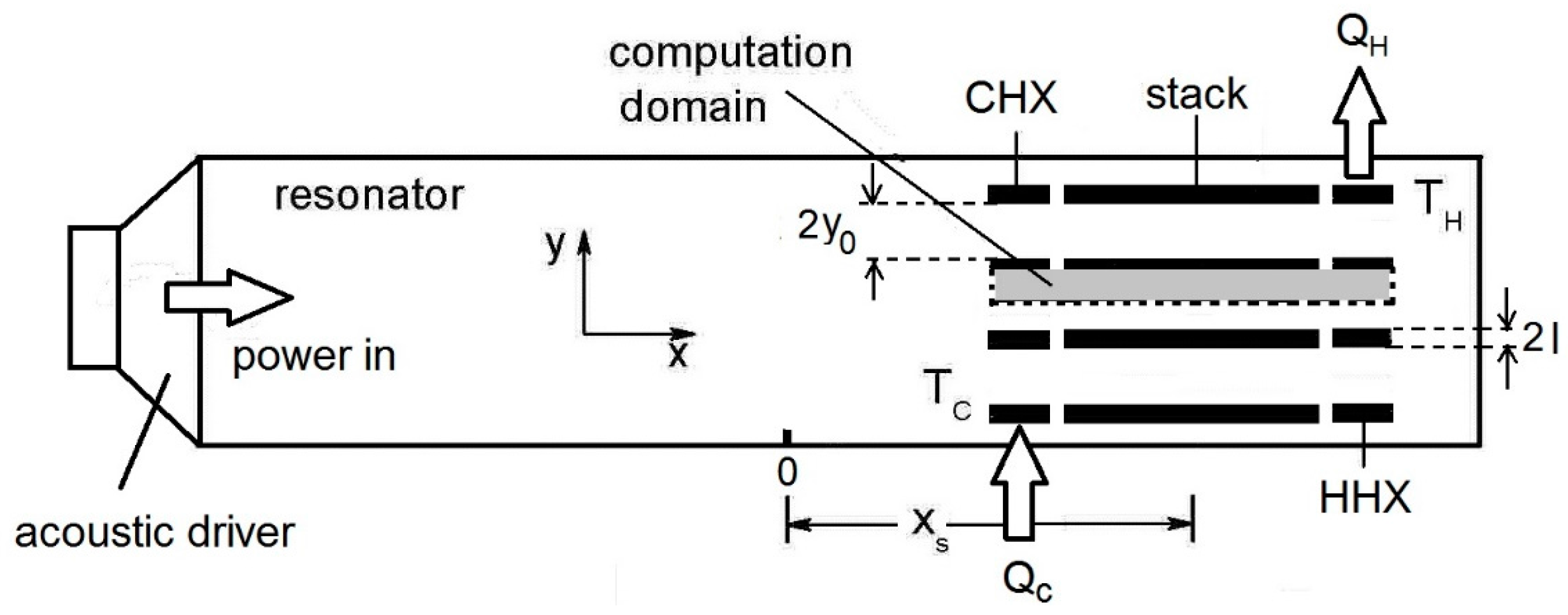
The modeled system is a stack of parallel plates, of length, L_S, sandwiched between “hot” and “cold” parallel-fin HXs of length L_H and L_C respectively. These last are treated as two isothermal surfaces maintained at temperature T_H and T_C. The stack-HXs assembly is located at a distance x_s from the center of a half-wavelength (λ/2) gas filled resonator sustaining a standing acoustic wave as shown in Figure 1. The system is supposed to work in the refrigeration mode so heat is pumped from the cold to the hot HX through the stack along the positive longitudinal x direction (see Figure 1). To simplify numerical implementation stack plates and HX fins are modeled with the same spacing (2y₀) and thickness (2l) with the HX fins aligned to the stack plates and separated from them by a small finite gap (in order to reduce adverse heat conduction leaks from the cold to the hot HX).The periodicity of the stack and HXs structures along the transverse direction normal to the plates/fins (the y direction) allows calculations to be performed in a single channel of the stack-HXs assembly and in the couple of plates/fins enclosing it. The computational domain is further reduced by symmetry from half a gas duct to half a plate/fin as indicated by the light grey area together with the coordinate system used (y = 0 is at the center of the fluid gap).

Figure 1. Schematic illustration of the modeled thermoacoustic refrigerator with magnified view of the simulation domain (grey area). Plate interspacing and thickness are not in scale.

Figure 1. Schematic illustration of the modeled thermoacoustic refrigerator with magnified view of the simulation domain (grey area). Plate interspacing and thickness are not in scale.

As for the acoustic field, the stack is considered to be significantly shorter than the acoustic wavelength and not intrusive so that the oscillating pressure and velocity can be described in the stack-HXs neighbourhood by a 1D lossless standing wave:

$$\begin{array}{ccc}{p}_1=P_A \text{sin} ({kx}_s)=p_0& & v_{x1}=j\frac{P_A}{{\rho }_{0}a}\text{cos} ({kx}_s)=j{v}_0\end{array}$$

(1)

where p₁ is the amplitude of the dynamic pressure, P_A is the amplitude of the dynamic pressure at a pressure antinode, v_x1 is the amplitude of the longitudinal particle velocity, k is the wave number (k = 2π/λ) and a is the sound velocity. As emphasized by Swift [1], this approximation (the “short-stack” approximation) should be not too restrictive. Equations derived under this simplifying assumption should be able to describe the performance of realistic devices within about a factor of 2.

The gas temperature field is governed by the general equation of energy conservation [9] whose time averaged (over one or more acoustic cycles) version is:

$$\nabla \cdot \overline{\mathbf{e}}=0$$

(2)

where $\overline{\mathbf{e}}$ is the energy flux density vector and where over-bar means time-averaged variable. In our 2D model we consider only the x and y components of $\overline{\mathbf{e}}$ [10]:

$${\overline{e}}_x=\frac{\omega }{2\pi }\left({\displaystyle \underset{0}{\overset{2\pi /\omega }{\int }}}{\rho v}_x\left(\frac{1}{2}{v}^2+h\right)dt-{\displaystyle \underset{0}{\overset{2\pi /\omega }{\int }}}(v_x{\sigma }_{xx}+v_y{\tau }_{xy}) dt-K{\displaystyle \underset{0}{\overset{2\pi /\omega }{\int }}}\frac{\partial T}{\partial x} dt\right)$$

(3)

$${\overline{e}}_y=\frac{\omega }{2\pi }\left({\displaystyle \underset{0}{\overset{2\pi /\omega }{\int }}\rho v_y\left(\frac{1}{2}{v}^2+h\right)dt}-{\displaystyle \underset{0}{\overset{2\pi /\omega }{\int }}(v_x{\tau }_{xy}+v_y{\sigma }_{yy}) dt}-K{\displaystyle \underset{0}{\overset{2\pi /\omega }{\int }}\frac{\partial T}{\partial y} dt}\right)$$

(4)

where ω is the angular frequency, ρ is the gas density, h is the specific enthalpy, t is the time, K is the gas thermal conductivity, v is the velocity (whose components are v_x and v_y), T is the temperature and:

$${\sigma }_{xx}=\frac{2}{3}\eta \left(2\frac{\partial v_x}{\partial x}-\frac{\partial v_y}{\partial y}\right)\approx -\frac{2}{3}\eta \frac{\partial v_y}{\partial y}$$

(5)

$${\tau }_{xy}={\tau }_{yx}=\eta \left(\frac{\partial v_x}{\partial y}+\frac{\partial v_y}{\partial x}\right)\approx \eta \frac{\partial v_x}{\partial y}$$

(6)

$${\sigma }_{yy}=\frac{2}{3}\eta \left(2\frac{\partial v_y}{\partial y}-\frac{\partial v_x}{\partial x}\right)\approx \frac{4}{3}\eta \frac{\partial v_y}{\partial y}$$

(7)

are the components of the viscous stress tensor. In the last expressions the x velocity gradients have been disregarded, being of order δv/λ smaller than the y velocity gradients ((δv = 2η/ρ₀ω)^1/2 being the “viscous penetration depth” whose definition includes the shear viscosity coefficient, η, the static density, ρ₀, and ω). To proceed further we observe that in the low Mach number regime (considered in this work) any acoustic variable ξ can be expressed in complex notation by the conventional first-order expansion ξ(x,y,t) = ξ₀(x,y) + Re{ ξ₁(x,y)e^jωt} where j is the imaginary unit, ξ₀ is the (real) mean value, ξ₁ the (complex) amplitude of oscillation and where Re{ }denotes the real part. Making use of this notation and retaining only terms up to second order Equations (3) and (4) become:

$${\overline{e}}_x=\frac{1}{2}{\rho }_0{c}_P\text{Re}\{T_1 {\tilde{v}}_{x1}\}+\frac{1}{3}\eta \text{Re}\left\{\frac{\partial v_{y1}}{\partial y}{\tilde{v}}_{x1}\right\}-\frac{1}{2}\eta \text{Re}\left\{\frac{\partial {\tilde{v}}_{x1}}{\partial y}{v}_{y1}\right\}-K\frac{\partial T_0}{\partial x}$$

(8)

$${\overline{e}}_y=\frac{1}{2}{\rho }_0{c}_P\text{Re}\{T_1 {\tilde{v}}_{y1}\}-\frac{1}{2}\eta \text{Re}\left\{\frac{\partial v_{x1}}{\partial y}{\tilde{v}}_{x1}\right\}-\frac{2}{3}\eta \text{Re}\left\{\frac{\partial v_{y1}}{\partial y}{\tilde{v}}_{y1}\right\}-K\frac{\partial T_0}{\partial y}$$

(9)

where T₁ is the amplitude of the oscillating temperature, c_p is the isobaric specific heat of the gas, T₀ is the time-averaged temperature, v_x1 is the amplitude of the longitudinal velocity, v_y1 is the amplitude of the transverse velocity and where tilde indicates complex conjugation. The explicit expressions of these equations to be implemented in the model are obtained by substitution of the standard equations of the classical thermoacoustic theory for T₁, v_x1, ∂v_x1/∂y, v_y1 and ∂v_y1/∂y inside a gas pore [1,7,8,9], where the longitudinal pressure gradient dp₁/dx at the stack location is calculated by imposing the continuity of the volume flow rate at the entrance of the stack/HXs assembly through the equation:

$$\frac{d{p}_1}{dx}=\frac{{\rho }_0 \omega }{( 1-f_{\nu }) BR}{v}_0$$

(10)

The result is:

$${\overline{e}}_x=A_x(y)-B_x(y)\frac{\partial T_0}{\partial x}-K\frac{\partial T_0}{\partial x} {\overline{e}}_y=A_y(y)+B_y(y)\frac{\partial T_0}{\partial x}+C_y(y){\left(\frac{\partial T_0}{\partial x}\right)}^2-K\frac{\partial T_0}{\partial y}$$

(11)

where:

$$A_x(y)=\frac{1}{2\text{BR}}\text{Im} \left\{\frac{{\mathsf{\Pi }}_1{\tilde{\mathsf{\Pi }}}_2}{(1-{\tilde{f}}_{\nu })}\right\}{P}_0 v_0+\frac{\eta \omega }{3\text{BR}{\rho }_0{a}^2}\text{Re} \left\{\frac{{\tilde{\mathsf{\Pi }}}_2{\mathsf{\Pi }}_5}{(1-{\tilde{f}}_{\nu })}\right\}{p}_0 v_0+\frac{\eta \omega }{{\rho }_0\text{BR}{a}^2{\delta }_{\nu }^2}\text{Im}\left\{\frac{{\tilde{k}}_{\nu }{\mathsf{\Pi }}_3}{(1-{\tilde{f}}_{\nu })}\right\}{p}_0{v}_0$$

(12)

$$\begin{array}{ll}{B}_x(y)& =\frac{{\rho }_0{c}_P}{2 \omega {\text{BR}}^2(1-\text{Pr}){|1-f_{\nu }|}^2}\text{Im}\left\{{\mathsf{\Pi }}_1{\tilde{\mathsf{\Pi }}}_2\right\} v_0^2-\frac{\eta \beta }{3{\text{BR}}^2(1-\text{Pr}){|1-f_{\nu }|}^2}\text{Re}\left\{{\tilde{\mathsf{\Pi }}}_2{\mathsf{\Pi }}_6\right\}{v}_0^2\\ & -\frac{\eta \beta }{{\delta }_{\nu }^2{\text{BR}}^2(1-\text{Pr}){|1-f_{\nu }|}^2}\text{Im}\left\{{\tilde{k}}_{\nu }{\mathsf{\Pi }}_4\right\} v_0^2\end{array}$$

(13)

$$A_y(y)=\frac{\omega }{2{\rho }_0 a^2}\text{Im}\left\{{\mathsf{\Pi }}_1{\tilde{\mathsf{\Pi }}}_3\right\}{p}_0^2-\frac{\eta }{{\text{BR}}^2{\delta }_{\nu }^2{|1-f_{\nu }|}^2}\text{Im} \left\{k_{\nu }{\tilde{\mathsf{\Pi }}}_2\right\} v_0^2-\frac{2\eta {\omega }^2}{3{\rho }_0^2{a}^4}\text{Re}\left\{{\tilde{\mathsf{\Pi }}}_3{\mathsf{\Pi }}_5\right\}{p}_0^2$$

(14)

$$\begin{array}{ll}{B}_y(y)& =\frac{\beta }{2\text{BR}(1-\text{Pr})}\text{Im}\left\{\frac{{\mathsf{\Pi }}_1{\tilde{\mathsf{\Pi }}}_4}{(1-{\tilde{f}}_{\nu })}\right\}{p}_0{v}_0+\frac{c_p}{2\text{BR} (1-\text{Pr})a^2}\text{Re}\left\{j\frac{({\mathsf{\Pi }}_1-\text{Pr}{\mathsf{\Pi }}_2){\tilde{\mathsf{\Pi }}}_3}{(1-f_{\nu })}\right\}{p}_0{v}_0\\ & -\frac{2\eta \beta \omega }{3{\rho }_0\text{BR} a^2(1-\text{Pr})}\text{Re}\left\{\frac{{\tilde{\mathsf{\Pi }}}_4{\mathsf{\Pi }}_5}{(1-{\tilde{f}}_{\nu })}+\frac{{\tilde{\mathsf{\Pi }}}_3{\mathsf{\Pi }}_6}{(1-f_{\nu })}\right\}{p}_0{v}_0\end{array}$$

(15)

$$C_y(y)=\frac{\beta {\rho }_0 c_p}{2\omega {\text{BR}}^2{(1-\text{Pr})}^2 |1-f_{\nu }{|}^2}\text{Re}\{j({\mathsf{\Pi }}_1-\text{Pr}{\mathsf{\Pi }}_2){\tilde{\mathsf{\Pi }}}_4\}{v}_0^2-\frac{2\eta {\beta }^2}{3{\text{BR}}^2{(1-\text{Pr})}^2 |1-f_{\nu }{|}^2}\text{Re}\left\{{\tilde{\mathsf{\Pi }}}_4{\mathsf{\Pi }}_6\right\} v_0^2$$

(16)

$${\mathsf{\Pi }}_1=(1-h_{\kappa }) {\mathsf{\Pi }}_2=(1-h_{\nu })$$

(17)

$${\mathsf{\Pi }}_3=\frac{\left[1+(\gamma -1)f_{\kappa }\right] (y-k_{\nu })-\left[y+(\gamma -1)k_{\kappa }\right] (1-f_{\nu })}{(1-f_{\nu })} {\mathsf{\Pi }}_4=\frac{f_{\nu }(y-k_{\kappa })-f_{\kappa }(y-k_{\nu })+(k_{\kappa }-k_{\nu })}{(1-f_{\nu })}$$

(18)

$${\mathsf{\Pi }}_5=\frac{\left[1+(\gamma -1)f_{\kappa }\right] (1-h_{\nu })-\left[1+(\gamma -1)h_{\kappa }\right] (1-f_{\nu })}{(1-f_{\nu })} {\mathsf{\Pi }}_6=\frac{f_{\nu }(1-h_{\kappa })-f_{\kappa }(1-h_{\nu })+(h_{\kappa }-h_{\nu })}{(1-f_{\nu })}$$

(19)

$$h_{\kappa }=\frac{\text{cosh} \left[(1+j)y/{\delta }_{\kappa }\right]}{\text{cosh} \left[(1+j)y_0/{\delta }_{\kappa }\right]} h_{\nu }=\frac{\text{cosh} \left[(1+j)y/{\delta }_{\nu }\right]}{\text{cosh} \left[(1+j)y_0/{\delta }_{\nu }\right]}$$

(20)

$$k_{\kappa }=\frac{{\delta }_{\kappa }}{1+j}\frac{\text{sinh}\left[(1+j)y/{\delta }_{\kappa }\right]}{\text{cosh}\left[(1+j)y_0/{\delta }_{\kappa }\right]} k_{\nu }=\frac{{\delta }_{\nu }}{1+j}\frac{\text{sinh}\left[(1+j)y/{\delta }_{\nu }\right]}{\text{cosh}\left[(1+j)y_0/{\delta }_{\nu }\right]}$$

(21)

$$f_{\kappa }=\frac{\text{tanh}\left[( 1+j)y_0/{\delta }_{\kappa }\right]}{\left[( 1+j)y_0/{\delta }_{\kappa }\right]} f_{\nu }=\frac{\text{tanh}\left[( 1+j)y_0/{\delta }_{\nu }\right]}{\left[( 1+j)y_0/{\delta }_{\nu }\right]}$$

(22)

and where the “blockage ratio” BR = A/A_dct = 1/(1 + l/y₀) describes the porosity of the stack-HXs assembly (A_dct being the cross sectional area of the resonator duct and A the cross sectional area of the stack-HXs assembly open to gas flow), β is the gas thermal expansion coefficient, Pr is the Prandtl number, δk = (2K/ρ_0Cpω))^1/2 is the “thermal penetration depth” and where Im{ } denotes the imaginary part. We note that these energy flux densities can be identified with heat flux densities because in the short stack approximation the work flux contribution to the total energy flux is small [1]. The energy fluxes along the x and y directions inside the solid plates/HXs are expressed through the Fourier law since heat conduction is here the relevant mechanism of energy transport.

The calculation of the steady-state two-dimensional time-averaged temperature distribution both in the gas and in the solid is performed using a finite difference methodology where temperature spatial gradients are discretized using first order nodal temperature differences. To this end, the computational domain is subdivided using a rectangular grid. In the x direction the computation mesh size is typically 0.005 L_S while in the y direction the computation mesh size is typically 0.02 y₀.

The imposed boundary conditions took into account:

(a)

the symmetry on the central lines of a gas pore (y = 0) and of a solid plate/fin (y = y₀ + l)

$${\left(\frac{\partial T_0}{\partial y}\right)}_{y=0}={\left(\frac{\partial T_0}{\partial y}\right)}_{y=y_0+l}=0$$

(23)

(b)

the continuity of temperature and transverse heat fluxes at the gas-solid interfaces (y = y₀):

$$\begin{array}{ccc}{T_0|}_{gas}(y=y_0)={T_0|}_{solid}(y=y_0)& & K{\left(\frac{\partial T_0}{\partial y}\right)}_{y=y_0}=K_{solid}{\left(\frac{\partial T_0}{\partial y}\right)}_{y=y_0}\end{array}$$

(24)

K_solid being the thermal conductivity of the solid material (stack plates or HX fins);

(c)

the vanishing heat flux at the HX fin terminations (y₀ ≤ y ≤ y₀ + l) facing the resonator duct and at the HX pore ends (0 ≤ y ≤ y₀) facing the resonator duct (gas oscillations outside the HXs are adiabatic and thus the thermoacoustic effect vanishes):

$${\left(\frac{\partial T_0}{\partial x}\right)}_{x=0}={\left(\frac{\partial T_0}{\partial x}\right)}_{x=(L_C+L_S+L_H)}=0 {\overline{e}}_x(x=0)={\overline{e}}_x(x=L_C+L_S+L_H)=0$$

(25)

As for the separation gap between the HX fin and the stack edge, this last was arbitrarily set equal to δk and, as a further simplifying hypothesis, the slice of gas enclosed in it is assumed at rest. Applying Equation (2) to impose local energy balance in each cell of the computational grid, a system of quadratic algebraic equations with respect of the unknown variable T₀ is generated. The system is solved by a code developed by the author in FORTRAN-90 language which executes the recursive Newton-Raphson method [11]. At each iteration the system of linear algebraic equations providing the temperature corrections for the next step is solved using a LU decomposition with partial pivoting and row interchanges matrix factorization routine. The latter is taken from the LAPACK library routines available online at [12], where details about accuracy, computation cost, etc. can be found.

Once the time-averaged temperature distribution is known, it can be substituted in Equation (11) and in the Fourier law to determine the energy flux distributions along the x and y directions both in the gas and in the solid plates/fins and other relevant variables. Specifically, in this work it is used to calculate ${\overline{s}}_{\kappa }$—the time-averaged entropy generation rate per unit volume due heat transfer irreversibility (including thermal dissipation), and ${\overline{s}}_{\nu }$—the time-averaged entropy generation rate per unit volume due to fluid friction irreversibility (neglecting bulk viscosity) through the formulas [10]:

$${\overline{s}}_{\kappa }=\frac{\omega }{2\pi }{\displaystyle \underset{0}{\overset{2\pi /\omega }{\int }} s_{\kappa }} dt=\frac{\omega }{2\pi }{\displaystyle \underset{0}{\overset{2\pi /\omega }{\int }} \frac{K{(\nabla T)}^2}{T^2}} dt=\frac{K}{T_0^2}\left[{\left(\frac{\partial T_0}{\partial x}\right)}^2+{\left(\frac{\partial T_0}{\partial y}\right)}^2+\frac{1}{2}{\left|\frac{\partial T_1}{\partial y}\right|}^2\right]$$

(26)

$${\overline{s}}_{\nu }=\frac{\omega }{2\pi }{\displaystyle \underset{0}{\overset{2\pi /\omega }{\int }}{s}_{\nu } dt}=\frac{\omega }{2\pi }{\displaystyle \underset{0}{\overset{2\pi /\omega }{\int }}\frac{\eta }{T}\mathsf{\Phi } dt}=\frac{\eta }{T_0}\left[\frac{1}{2}{\left|\frac{ \partial v_{x1}}{\partial y}\right|}^2+\frac{2}{3}{\left|\frac{ \partial v_{y1}}{\partial y}\right|}^2\right]$$

(27)

having neglected, as before, the longitudinal temperature and velocity gradients respect to the transverse ones and where Ф, the dissipation term, has the following expression [10]:

$$\mathsf{\Phi }={\left(\frac{\partial v_x}{\partial y}+\frac{\partial v_y}{\partial x}\right)}^2+2{\left(\frac{\partial v_x}{\partial x}\right)}^2+2{\left(\frac{\partial v_y}{\partial y}\right)}^2-\frac{2}{3}{\left(\frac{\partial v_x}{\partial x}+\frac{\partial v_y}{\partial y}\right)}^2$$

(28)

Making use again of the standard equations of the classical thermoacoustic theory for T₁, v_x1, ∂v_x1/∂y, v_y1 and ∂v_y1/∂y with:

$$\frac{\partial T_1}{\partial y}=-j\frac{2 k_{\kappa }}{{\rho }_0 c_p {\delta }_{\kappa }^2}{p}_1-j\frac{2 (k_{\nu }-k_{\kappa })}{{\rho }_0 {\omega }^2 {\delta }_{\kappa }^2 (1-\text{Pr})}\frac{\partial T_0}{\partial x}\frac{d{p}_1}{dx}$$

(29)

Equations (26) and (27) can be put in the form:

$$\begin{array}{ll}{\overline{s}}_{\kappa }& =\frac{K}{T_0^2}[{\left(\frac{\partial T_0}{\partial x}\right)}^2+{\left(\frac{\partial T_0}{\partial y}\right)}^2+\frac{2{\left|k_{\kappa }\right|}^2}{{\rho }_0^2{c}_p^2{\delta }_{\kappa }^4}{p}_0^2+\frac{4}{{\rho }_0{c}_p\omega \mathsf{\Omega }(1-\text{Pr}){\delta }_{\kappa }^4}\frac{\partial T_0}{\partial x}\text{Re}\left\{\frac{k_{\kappa }({\tilde{k}}_{\nu }-{\tilde{k}}_{\kappa })}{1-{\tilde{f}}_{\nu }}\right\}{p}_0{v}_0\\ & +\frac{2}{{\omega }^2{\mathsf{\Omega }}^2{\delta }_{\kappa }^4{(1-\text{Pr})}^2}\frac{{\left|k_{\nu }-k_{\kappa }\right|}^2}{{\left|1-f_{\nu }\right|}^2}{\left(\frac{\partial T_0}{\partial x}\right)}^2{v}_0^2]\end{array}$$

(30)

$$\begin{array}{ll}{\overline{s}}_{\nu }& =\frac{\eta }{T_0}[\frac{2}{{\mathsf{\Omega }}^2{\delta }_{\nu }^4}\frac{{\left|k_{\nu }\right|}^2}{{\left|1-f_{\nu }\right|}^2}{v}_0^2+\frac{2{\omega }^2}{3{\rho }_0^2{a}_0^4}{\left|{\mathsf{\Pi }}_w\right|}^2{p}_0^2+\frac{4\beta \omega }{3{\rho }_0{a}_0^2\mathsf{\Omega }(1-\text{Pr})}\frac{\partial T_0}{\partial x}\text{Re}\left\{\frac{{\mathsf{\Pi }}_5{\tilde{\mathsf{\Pi }}}_6}{1-{\tilde{f}}_{\nu }}\right\}{p}_0{v}_0\\ & +\frac{2{\beta }^2}{3{\mathsf{\Omega }}^2{(1-\text{Pr})}^2{\left|1-f_{\nu }\right|}^2}{\left(\frac{\partial T_0}{\partial x}\right)}^2{\left|{\mathsf{\Pi }}_6\right|}^2{v}_0^2]\end{array}$$

(31)

suitable for calculation.

Once local entropy generation rates are obtained, they can be conveniently integrated over an arbitrary control volume V to obtain volume averaged entropy changes:

$$<{\overline{s}}_{\kappa }> =\frac{1}{V}{\displaystyle \underset{V}{\int }{\overline{s}}_{\kappa } dV} <{\overline{s}}_{\nu }> =\frac{1}{V}{\displaystyle \underset{V}{\int }{\overline{s}}_{\nu } dV}$$

(32)

(where brackets < > indicate a volume-averaged quantity) or the total time averaged entropy generation in a component (stack or HXs) as:

$${({\overline{S}}_{\kappa })}_s=\text{BR}{A}_{dct}{L}_s<{\overline{s}}_{\kappa }{>}_s {({\overline{S}}_{\kappa })}_{HHX}=\text{BR}{A}_{dct}{L}_H<{\overline{s}}_{\kappa }{>}_{HHX} {({\overline{S}}_{\kappa })}_{CHX}=\text{BR}{A}_{dct}{L}_C<{\overline{s}}_{\kappa }{>}_{CHX}$$

(33)

$${({\overline{S}}_{\nu })}_s=\text{BR}{A}_{dct}{L}_s<{\overline{s}}_{\nu }{>}_s {({\overline{S}}_{\nu })}_{HHX}=\text{BR}{A}_{dct}{L}_H<{\overline{s}}_{\nu }{>}_{HHX} {({\overline{S}}_{\nu })}_{CHX}=\text{BR}{A}_{dct}{L}_C<{\overline{s}}_{\nu }{>}_{CHX}$$

(34)

where subscripts “s”, “HHX” and “CHX” refer to the stack, hot HX and cold HX, respectively. Previous validation of the model against experimental data and results of analogous computational models can be found in [7,9].

3. Results and Discussion

In the optimization procedure of the HXs a standing-wave thermoacoustic device working in the refrigeration mode is considered. The configuration parameters are arbitrarily selected, even if they broadly respond to well known design criteria such as the use of low-Prandtl noble gases, high static pressures, stack located in proximity of the pressure antinode to reduce viscous dissipation, stack plate interspacing ranging between 2 and 4 δ_k, etc.. Helium at a static pressure of 3 bar and at a mean temperature of 300 K is assumed as working fluid (η = 199 × 10⁻⁷ N·s·m⁻², K = 0.152 W·m⁻¹·K⁻¹, a = 1008 m·s⁻¹, Pr = 0.68 at T = 300 K). It is considered enclosed in a half-wavelength resonator (acoustic wavelength λ = 6 m) resonating at 168 Hz (for which δ_k = 3.39 × 10⁻⁴ m) and having a circular cross section of radius 0.05 m Supposedly, the stack is in stainless steel (K_S = 14.9 W·m⁻¹·K⁻¹ at 300 K) while the HXs material is copper (K_copper = 401 W·m⁻¹·K⁻¹ at 300 K). In all runs the following parameters were fixed to the following constant values: (a) drive ratio (the ratio of the dynamic pressure amplitude in a pressure antinode to the static pressure) DR = 8.33%; (b) stack position x_S = 1.3 m; (c) stack length L_S = 0.13 m; (d) temperature of the cold HX T_C = 273.16 K; (e) temperature of the hot HX T_H = 300 K. For these operating conditions the dynamic Reynolds number (v_x1δvρ₀/η) and Mach number (P_A/ρ₀a²) resulted always smaller than 500 and 0.1 respectively, the values over which turbulence and non-linear saturation effects are expected to affect fluid dynamics [1].

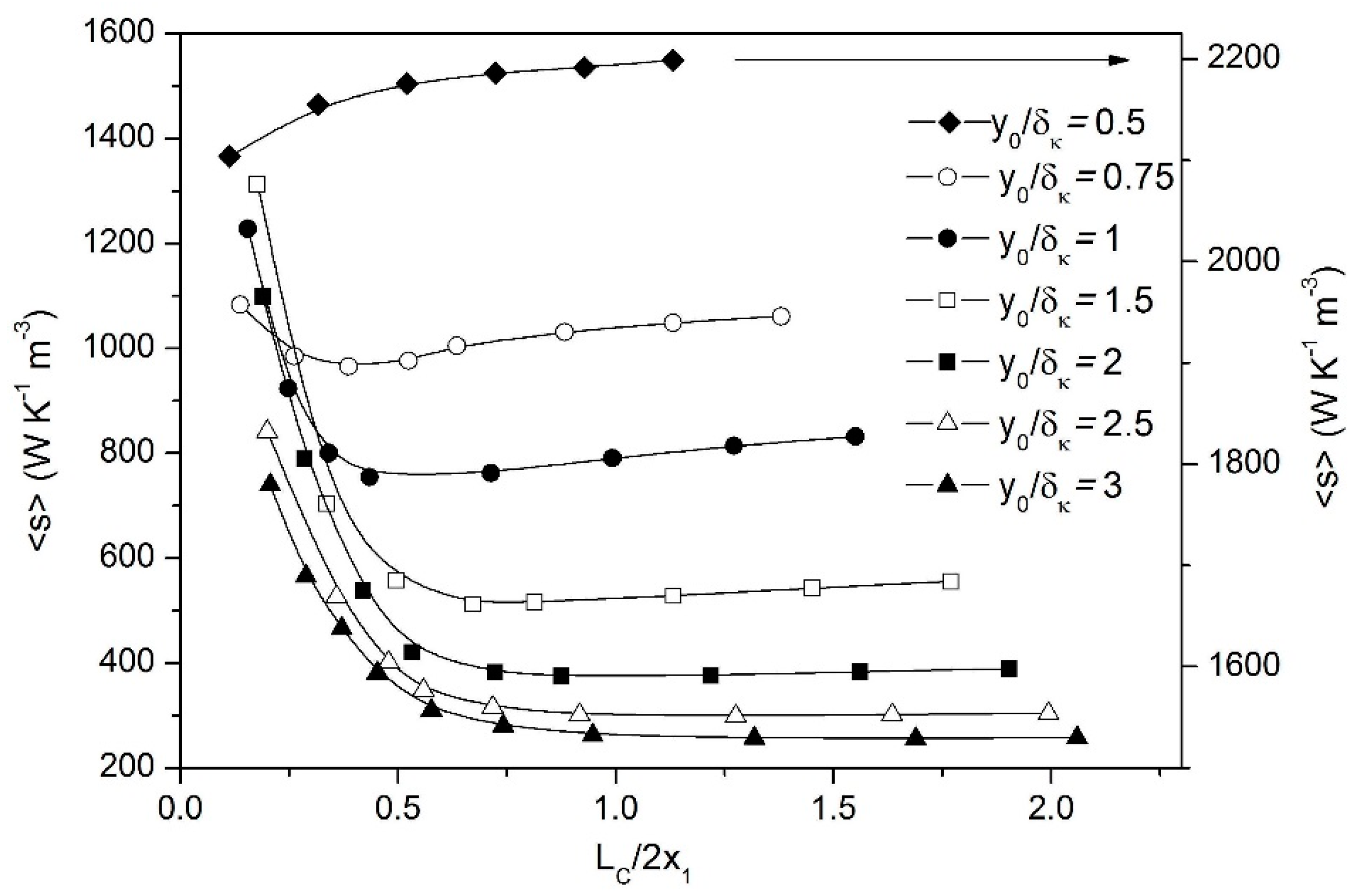
The dependence of the entropy generation on fin spacing and length can be observed in Figure 2, where the entropy generation rate per unit volume $<\overline{s}>$ averaged over the cold HX is plotted as a function of the fin length L_C at selected fin interspacing. In each run L_H was held fixed to 2x₁, the peak-to-peak particle displacement amplitude (consistently with the argument put forward by Swift [1]). The strong dependence of $<\overline{s}>$ on L_C at small L_C values is caused essentially by the thermal diffusion term: the increase of the fin length or, equivalently, of the surface area available for heat transfer decreases, in fact, the transverse temperature gradients required to sustain the heat flux. The viscous term does not contribute to the variation of $<\overline{s}>$ with L_C since the dissipation due to viscous friction is proportional to the fin area which, in turn is proportional to L_C and we are considering entropy generation values normalized by the volume enclosed between two fins. Conversely, the strong dependence of $<\overline{s}>$ on y₀ for y₀ < δ_k ( ≈ δv) is mainly due to the viscous term since viscous dissipation maximizes for for y → 0 (on the fin surface) and since the velocity (and associated viscous dissipation) grows ad decreasing y₀ values. This fact is clearly reflected by the monotonic growth with L_C of the curve at y₀ = 0.5 δ_k where the viscous term dominates over the thermal diffusion term. At y₀ ≈ δ_k the thermal diffusion term is comparable (or overcomes) the viscous one since the thermal dissipation maximizes at the distance y₀ = δ_k from the plate as well as the thermoacoustic heat transport which causes an increase of the transverse temperature gradients at the HXs. The trend for y₀ > δ_k simply reflects the circumstance that the thermal and viscous dissipation are relevant only within the thermal and viscous boundary layers. Finally, an interesting feature observable in Figure 2 is the existence of minima in correspondence of fin lengths of the order of the particle displacement amplitude at almost all the y₀ values considered. If the minimum of each curve is selected as optimal HX fin length, this last results to be an increasing function of the fin spacing.

Figure 2. The entropy generation rate per unit volume averaged over the cold HX as a function of the fin length L_C at selected fin spacing. Continuous lines are a guide for the eye.

Figure 2. The entropy generation rate per unit volume averaged over the cold HX as a function of the fin length L_C at selected fin spacing. Continuous lines are a guide for the eye.

The strong dependence of the entropy generation rate on both the fin length and the fin spacing suggests that minimization in entropy generation could constitute an effective design criteria for selecting the optimal HXs configuration in correspondence of given operating conditions. In this work this design strategy is applied to the model system under study by undertaking a parametric analysis of the influence of the main geometric parameters of the HXs—namely, the fin interspacing 2y₀, the hot HX length L_H and the cold HX length L_C—on the entropy generation rates.

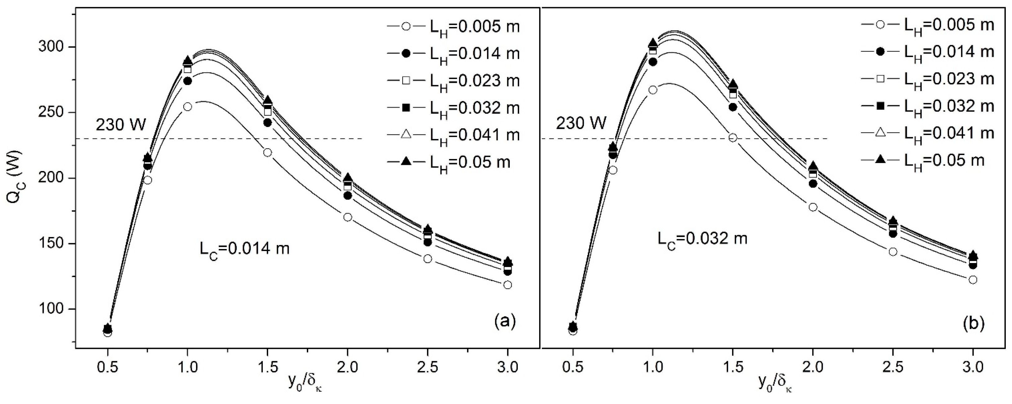
The analysis started by studying the dependence on L_C, L_H and y₀ of the total cooling rate $\overline{Q}$ sustained by the cold HX calculated as:

$${\overline{Q}}_C=\mathsf{\Pi }{\displaystyle \underset{0}{\overset{L_C}{\int }}K{\left(\frac{\partial T_0}{\partial y}\right)}_{y_0}dx}$$

(35)

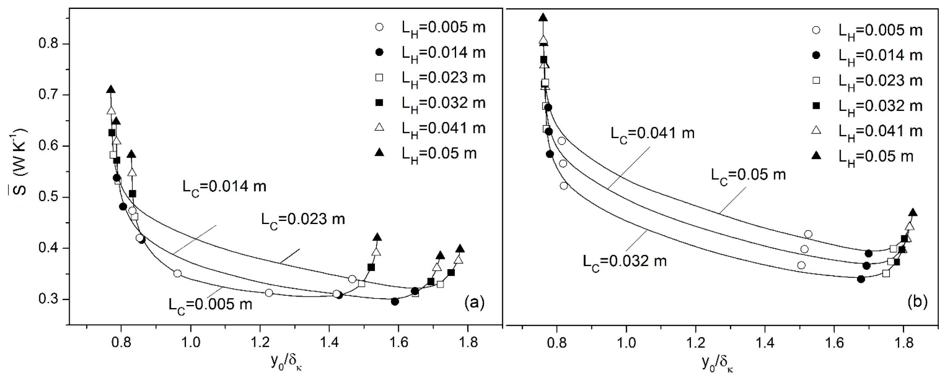
П being the perimeter of the cold HX cross section in contact with the gas. A typical result is shown in Figure 3a,b where ${\overline{Q}}_C$ is plotted as a function of y₀ for L_C fixed to 0.014 and 0.032 m and L_H ranging from 0.005 m to 0.05 m (note that 2x₁ = 0.0283 m for y₀ = 1.5 δ_k at the selected operation conditions). The graphs indicate that the optimal fin interspacing where the cooling power maximizes depends both on L_C and L_H simultaneously. The graphs also show that, for each fin length L_C, a given level of cooling power can be achieved by different combinations of L_H and y₀ values. In particular, for a given length of the cold HX, there are two fin interspacing values that could produce the desired refrigerating power.

Figure 3. The cooling power as a function of fin interspacing at selected lengths of the hot HX for L_C = 0.014 m (a) and L_C = 0.032 m (b). Continuous lines are a guide for the eye.

Figure 3. The cooling power as a function of fin interspacing at selected lengths of the hot HX for L_C = 0.014 m (a) and L_C = 0.032 m (b). Continuous lines are a guide for the eye.

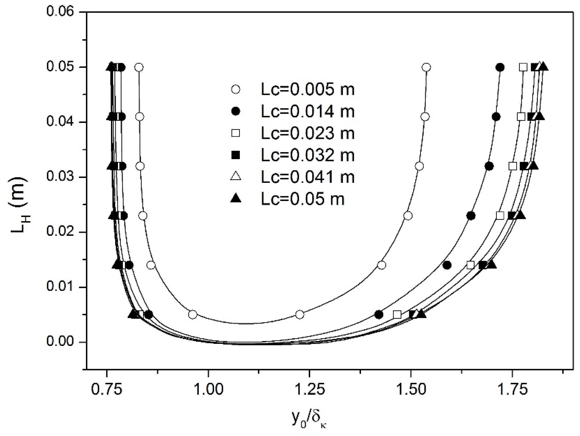
The second step of the procedure consisted in fixing a set point level for the cooling power and, subsequently, in determining the combinations of L_C, L_H and y₀ values giving rise to the above level.

The selected set point level for $\overline{Q}$ is indicated in Figure 3a,b by the horizontal dotted line and corresponds to ${\overline{Q}}_C$ = 230 W. The intercept of this line with the ${\overline{Q}}_C$ curves determines the combinations of L_H and y₀ values that produce the required cooling power at the considered L_C. The procedure has thus been repeated for all the L_C values considered (L_C = 0.005, 0.014, 0.023, 0.032, 0.041, 0.05). The results are summarized in Figure 4 where the relevant L_C, L_H and y₀ combinations are shown.

Figure 4. The combinations of L_C, L_H and y₀ values giving rise to a constant cooling power of 230 W at the selected operation point. Continuous lines are a guide for the eye.

Figure 4. The combinations of L_C, L_H and y₀ values giving rise to a constant cooling power of 230 W at the selected operation point. Continuous lines are a guide for the eye.

In the final step the total entropy generation rate was computed in the resulting combinations of L_C, L_H and y₀ values to find the existence of minima to be selected as favorable configurations for the HXs.

In these points the device should produce the desired output cooling level with minimum irreversibility (and best performance). Results are shown in Figure 5a,b where the entropy generation rate produced in all the stack-HXs assembly is reported as a function of the fin interspacing at selected L_C values (note that each curve is characterized by different L_H values). An inspection of the graphs reveals that for each length of the cold HX the entropy generation rate minimizes in correspondence of a unique combination of L_H, y₀ values. The lowest minimum, representing the best configuration for the HXs at the modeled operating conditions, is characterized by the values L_C ≈ L_H = x₁ and y₀/δ_k = 1.589. The important result found here is that the optimal HX fin length along the longitudinal direction is of the order of the gas displacement amplitude, a statement originally deduced by Swift on the basis of a Lagrangian picture of the inter-element heat transfer but recently confirmed by both numerical [12,13] and experimental [14,15] investigations.

Figure 5. The total time averaged entropy generation rate evaluated in the combinations of L_C, L_H and y₀ values producing an output cooling power equal to 230 W at the selected operation point. In (a) 0.005 m ≤ L_C ≤ 0.023 m. In (b) 0.032 m ≤ L_C ≤ 0.05 m. Continuous lines are a guide for the eye.

Figure 5. The total time averaged entropy generation rate evaluated in the combinations of L_C, L_H and y₀ values producing an output cooling power equal to 230 W at the selected operation point. In (a) 0.005 m ≤ L_C ≤ 0.023 m. In (b) 0.032 m ≤ L_C ≤ 0.05 m. Continuous lines are a guide for the eye.

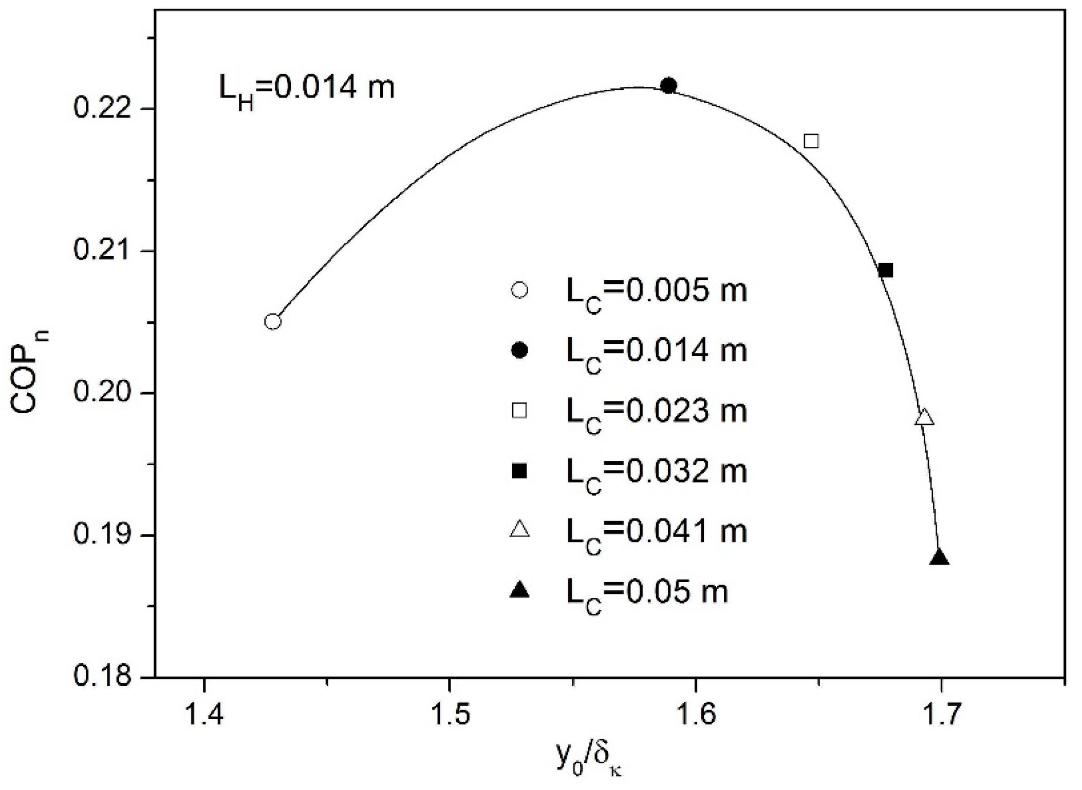
To verify if the performance of the device maximizes in correspondence of the optimal deduced configuration its coefficient of performance normalized by COP_C = T_C/(T_H − T_C) (the Carnot coefficient of performance) has been calculated in all the six minimum entropy configurations corresponding to the six investigated L_C values reported in Figure 5 as:

$$CO{P}_n=\frac{{\overline{Q}}_C/\overline{W}}{CO{P}_C}$$

(36)

where $\overline{W}$, the time-averaged total acoustic power absorbed in the entire stack-HXs assembly has been in turn calculated as:

$$\overline{W}={\displaystyle \underset{0}{\overset{y_0}{\int }}{\displaystyle \underset{0}{\overset{L}{\int }}\overline{w}dx dy}}$$

(37)

where L = L_C + L_S + L_H and where $\overline{w}$, the time-averaged acoustic power absorbed per unit volume by thermal expansion/contraction and viscous dissipation, is given by [1,7]:

$$\overline{w}=\omega \beta \overline{p_1(j{T}_1)}+\beta \left(\frac{\partial T_0}{\partial x}\right) \overline{p_1{v}_{x1}}+\beta \left(\frac{\partial T_0}{\partial y}\right) \overline{p_1{v}_{y1}}-\eta \mathsf{\Phi }$$

(38)

Results are reported in Figure 6 where it is observable how the COP_n exhibits a maximum in correspondence of the best HXs configuration previously deduced reaching the value 0.22. This result supports the conclusion that entropy generation minimization can be considered as a viable design strategy of HXs in thermoacoustic applications.

Figure 6. The normalized coefficient of performance COP_n evaluated in the combinations of L_C, L_H, y₀ producing, a minimum in entropy generation for an output cooling power of 230 W. Continuous line is a guide for the eye.

Figure 6. The normalized coefficient of performance COP_n evaluated in the combinations of L_C, L_H, y₀ producing, a minimum in entropy generation for an output cooling power of 230 W. Continuous line is a guide for the eye.

4. Conclusions

The performance of thermoacoustic HXs schematically modeled as set of parallel fins coupled to a stack of parallel plates of equal BR has been investigated through a 2D numerical model based on the classical linear thermoacoustic theory. The model has been able to put in evidence the strong dependence of the entropy generation rate on both the fin length and the fin spacing and the existence of minima in correspondence of fin lengths of the order of the particle displacement amplitude (at almost all the y₀ values considered). The different weight of the thermal and viscous irreversibilities affecting the HXs behavior has also been highlighted with the second one dominating at very low fin interspacing. Also important for design purposes is that entropy generation minimization criterion could be effectively employed for the simultaneous optimization of the two HXs (the fin spacing and length of each one). The procedure, applied in this study to a model device operating in the refrigeration mode, has allowed to find the optimal HXs configuration for which the COP_n maximizes. As for the settings which optimize the HX performance, the results of this study support the ones previously found in [7,9]: the optimal length of the HXs along the direction of the acoustic vibration results to be of the order of the gas displacement amplitude, being an increasing function of the fin spacing (tightly spaced fins require shorter lengths).

The simplified computational method proposed in this work suffers from several limitations. Particularly, the HXs are modeled as coupled to the stack in a configuration involving the same blockage ratio (with the HX fin aligned to the stack plate) while their arrangement in real thermoacoustic devices is more complex. Heat exchangers and stack/regenerators are generally characterized by different blockage ratios. The associated cross sectional discontinuity causes the junction sections be interested by complex flow patterns which actually increase the friction losses. Calculations integrated in the model are formulated for heat exchangers with parallel fins so, in its actual form, the model is applicable to heat exchangers of this type. The methodology, however, is general and can be extended to other HX configurations, previous reformulation of the equations. Work is currently in progress to extend the model in order to overcome this shortcomings.