Entropy Generation through Deterministic Spiral Structures in Corner Flows with Sidewall Surface Mass Injection

Abstract

Results are presented for an innovative computational procedure that predicts time-dependent instabilities and deterministic ordered structures in three-dimensional steady-state laminar boundary-layer flows. The flow configuration considered is a corner flow with sidewall surface mass injection into a horizontal boundary-layer flow. The equations for the velocity fluctuations are cast into a spectral Lorenz-type format and incorporated into the overall computational procedure for the three-dimensional flow. The non-linear time-dependent solutions of the spectral equations predict deterministic spectral ordered structures within spiral structures. Spectral analysis of these fluctuating solutions yields the resulting entropy generation rates resulting from the dissipation of the ordered structures. The results for the entropy generation rates indicate the prediction of a strong burst of ordered structures within the range of injection velocities studied. This new computational method is applicable to only selected thermal design processes.

1. Introduction

In a recent article (Isaacson [1]), computational results for the entropy generation rates occurring in a three-dimensional boundary layer structure formed in a corner boundary-layer flow environment were reported. In that article, the generation of the triggering cross flow velocities was attributed to the formation of a stream wise boundary layer along the corner sidewall. However, further calculations indicate that the actual cross wind velocities produced by the formation of the sidewall boundary layer are insufficient to trigger the observed deterministic structures, and that the required values for the triggering velocities are twice that produced by the sidewall laminar boundary layer flow. The computational results reported in that article used the higher levels of velocity, indicating the production of ordered structures and the resulting generation of entropy from the dissipation of the observed ordered structures. Therefore, it becomes necessary to study the effects of higher superimposed crosswind velocities on the entropy generation rates in the corner flow environment. The configuration to accomplish this analysis consists of a corner flow environment, with sidewall surface mass injection, with the mass injection uniform in the steam wise direction, along the sidewall at the intersection of the sidewall with the horizontal surface. This configuration is shown in Figure 1.

Figure 1. Schematic of the corner flow configuration is shown.

Figure 1. Schematic of the corner flow configuration is shown.

As an example of a flow environment of this kind, consider the flow in the forward region of a rectangular slot in the slotted-grain of a solid-propellant rocket motor. A laminar boundary layer is initiated along the floor of the cavity, while the burning propellant sidewall provides the injection of mass into the boundary layer. This flow environment would be modeled as shown in Figure 1. This article includes the following sections: in Section 2, we discuss the thermodynamic and transport processes required for the flow of air at a selected temperature and pressure. These thermo-transport properties are used throughout the computational process. In Section 3, we discuss the theoretical and computational characteristics of each of the computational modules included in the overall procedure. Section 4 presents selected results for each phase of the procedure and a discussion of the overall results for the entropy generation rates for each of the selected environments. Section 5 includes speculations from non-equilibrium thermodynamics concerning possible mechanisms involved in the transition of dissipative ordered structures into equilibrium thermodynamic states.

The article closes with a discussion of the results and final conclusions.

2. Selection of Heated Air as the Working Substance

The flow configuration we are simulating in this exploratory study is shown in Figure 1. The figure is intended to represent the corner flow in the entrance to a square channel in, for example, an industrial heating unit. In this section, we describe the characteristics of the working gas we use in our computational procedure.

The working gas is assumed to be heated air with the following thermodynamic and transport properties:

Air temperature, T:   1068.0 K

(1)

Static pressure, p:   0.912 × 10⁵ N/m²

(2)

Kinematic viscosity, ν:   1.51634 × 10⁻⁴ m²/s

(3)

It should be noted that the value for the kinematic viscosity used in this study is very similar to the values used in previous studies. The explanation for this is that a series of coupled, nonlinear time-dependent differential equations are included in the computational procedure. The solutions for such equations are very sensitive to the initial conditions imposed on the equations and are also sensitive to the control parameters applied in the solution. The solution of the steady-state boundary-layer equations that provides these control parameters is dependent on the particular value of the kinematic viscosity applied in the calculations. We have found that only a narrow range of kinematic viscosities yields the prediction of ordered structures from the computational procedure (see e.g., [1,2,3,4,5]). The range of appropriate values of kinematic viscosities has not been delineated and remains as work to be done. The next section provides a review and guide to the mathematical basis for each part of the analysis and references to the computer program listings used in the computational procedure.

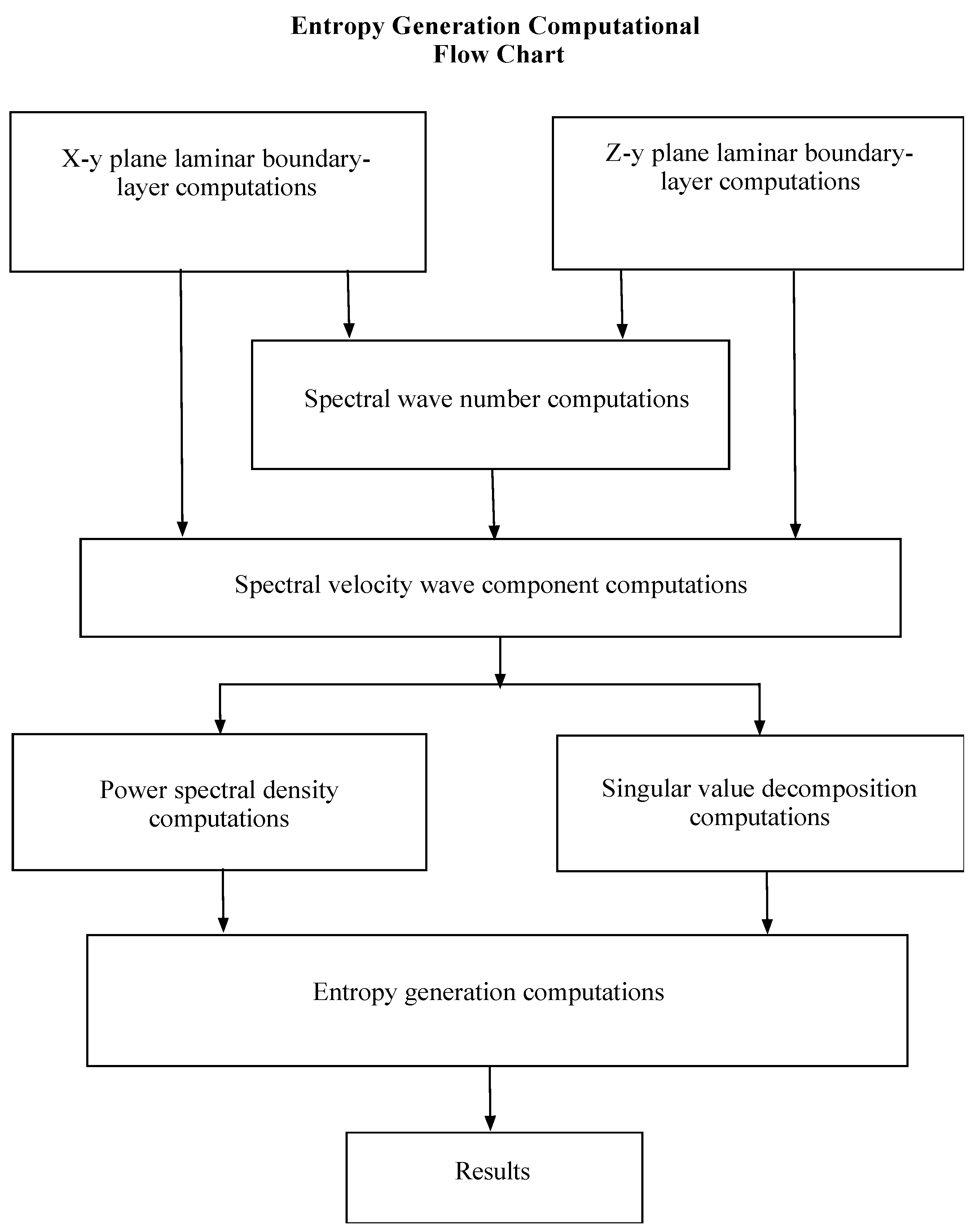
3. Review of Program Components

From the perspective of an overall view of the computational procedure used for the calculation of entropy generation rates, the process appears to be quite complicated. However, the solution of a complex problem is often accomplished by separating the process into solvable segments. This is the approach we have applied for the results presented in this article. This section describes each of these segments, with references to the original sources for the mathematical developments and the computer program listings. We have also included comments placing the subject of each particular segment in a non-equilibrium thermodynamics setting (Attard [6]).

3.1. Steady-Flow Boundary-Layer Development: Velocity Gradients

As indicated in Figure 1, the boundary-layer configuration consists of the boundary layer in the x-y plane produced by the stream wise velocity along the horizontal surface while the sidewall surface crosswind injection velocity provides the boundary layer in the z-y plane. These intersecting boundary layer profiles provide an orthogonal flow configuration. Hansen [7] has indicated that boundary layer profiles in such a coordinate system possess the characteristic of similarity, allowing for the introduction of the Falkner-Skan transformation (Cebeci and Bradshaw [8]) in the system of boundary layer equations. Cebeci and Bradshaw [8] present computer program listings for the numerical solutions for both laminar and turbulent boundary layers over horizontal surfaces. These program listings have been updated and extended to a broader range of problems in Cebeci and Cousteix [9]. The program listings used in the study reported here are those presented in [8]. The separation of the computation of the three-dimensional boundary-layer flow into the computation of the boundary-layer flow in the x-y plane and the computation of the boundary-layer flow in the z-y plane is one of the major approximations in the computational procedure. The rational for this approximation is that we are interested in the velocity gradients within the steady state boundary-layer profiles and similarity of the boundary layers should yield approximations for these profiles that are close to the three-dimensional results.

The equations required for the laminar boundary layer velocity gradients have been presented in [4]. These steady state boundary-layer velocity gradients serve as control parameters for the time-dependent solutions for the linear fluctuating spectral wave number components and the coupled, nonlinear Lorenz-type equations for the spectral velocity wave components.

In our thermodynamic system, the steady state boundary layer equations and the corresponding velocity gradients serve as the non-equilibrium thermodynamic steady state reservoir for the time-dependent development of the velocity fluctuations within the boundary layer environment (pp. 26–31, [6]). This reservoir provides the input control parameters for the time-dependent development of the spectral velocity fluctuations. The time-dependent part of the flow configuration is represented as a series of non-equilibrium sub-systems within the steady-state thermodynamic system. The phase space evolution of these sub-systems into a final equilibrium thermodynamic state is the subject of this article.

3.2. Modified Lorenz-Form Equations: Spectral Velocity Components

The crosswind velocity injected along the vertical sidewall surface produces a boundary layer along the horizontal surface in the z-y plane. The nonlinear interactions of this z-y boundary layer with the boundary layer in the x-y plane along the horizontal surface initiate time-dependent instabilities within the three-dimensional laminar boundary layer flow. A set of non-equilibrium, time-dependent equations in the spectral domain for these non-equilibrium instabilities, separate from the equations for the steady boundary layer flow, may be obtained through the methods of Townsend [10].

Isaacson [11] has presented the modifications of the time-dependent Townsend spectral equations into a linear set of equations for the spectral wave numbers and a set of coupled nonlinear equations for the fluctuating spectral velocity wave number components, written in a modified Lorenz format. The time-series solutions of the spectral wave number equations are dependent upon the initial conditions applied to the equations and on the complete set of steady-state boundary-layer velocity gradients obtained from the boundary layer solutions. These spectral wave number solutions are applied as control parameters in addition to the steady-state boundary layer velocity gradients to determine the time-series solutions of the modified Lorenz equations for the fluctuating spectral velocity wave number components at each stream wise station.

In the non-equilibrium thermodynamics context, the reservoir consists of the steady state velocity gradients with the time-series solution of the spectral wave numbers as sub-system 1. The nonlinear time series solutions for the spectral velocity wave number components in the spectral domain for each of the stream wise stations make up the remaining non-equilibrium thermodynamic sub-systems. Solutions of the overall set of equations are obtained at each of the six stream wise stations along the x-axis.

The application of these equations at the initial station requires that additional assumptions be applied to the modified Lorenz equations. Isaacson [11], Mathieu and Scott [12], and Manneville [13] have discussed both the format and justification for the particular choice of these assumptions for the initial station. The nonlinear time-series solutions of the modified Lorenz equations at the initial station are characterized as the non-equilibrium thermodynamic sub-system 2. These solutions contain the spectral velocity component fluctuations that we wish to study.

We wish to apply our computational procedure to the five remaining stations following the initial station along the stream wise direction. However, as Attard points out (pp. 42–45, [6]), we cannot just piece together a series of independent computations for each stream wise station. We must take into account that the nonlinear time series solutions obtained for the third and subsequent sub-systems will be influenced by the fluctuations produced in the previous sub-systems. To accomplish this, we introduce the synchronization properties of the modified Lorenz set of equations describing the nonlinear solutions for the spectral velocity wave number components (Isaacson [2,11]).

3.3. Synchronization Properties of the Modified Lorenz Equations

Pecora and Carroll [14], Pérez and Cerdeiral [15], and Cuomo and Oppenheim [16] have used the synchronization properties of systems of Lorenz-type equations to extract messages masked by chaotic signals. The synchronization properties of Lorenz-type equations are adapted here to extract ordered signals from the nonlinear time series generated for each of the spectral velocity wave components in the solution of the modified Lorenz equations.

As indicated previously, the solutions are obtained for a sequence of computational stations in the stream wise direction along the x-axis. We consider the initial station as the transmitter station. The following stations are considered as receiver stations. The various boundary layer coefficients at each of the receiver stations are computed in the same manner as in the transmitter station. Following the results in [2], the time-dependent output for the stream wise velocity wave vector component from the transmitter station is used as input to the nonlinear coupled terms in the modified Lorenz equations at the next station, which we denote as the first receiver station. Then, the input to the nonlinear-coupled terms at the next downstream receiver station is made up of the sum of the stream wise velocity wave component output from the transmitter station plus the stream wise velocity wave component output from the previous receiver station. This process is repeated for each of the five downstream receiver stations. With this method, the memory of the initial velocity fluctuations and the influence of subsequent fluctuations are retained in the overall computational procedure.

In the non-equilibrium thermodynamics context, the transmitter station is sub-system 2, with each of the successive stations as sub-system 3 through sub-system 7. The nonlinear time series solutions from the modified Lorenz equations for each of the non-equilibrium sub-systems will contain spectral velocity wave number fluctuations. These fluctuations will have both ordered and disordered regions dispersed within the time series [2]. We will use the power spectral density of these fluctuations to characterize the ordered regions within the fluctuations as described in [2].

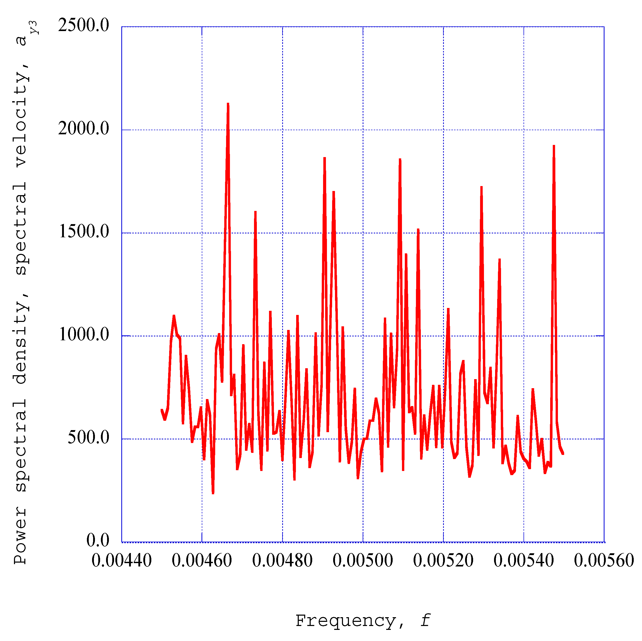
3.4. Power Spectral Density within the Deterministic Spectral Velocity Fluctuations

The Lorenz synchronization procedure yields the nonlinear time series solution for each of the five receiver stations in the stream wise direction. These solutions indicate the generation of deterministic spiral structures, with significant velocity fluctuations embedded within some of the time series solutions. Entropy generation through these spiral structures comes about by the dissipation of these fluctuations into equilibrium thermodynamic states. A fundamental requirement for the determination of the entropy generation is the characterization of the nature of these fluctuations. We have found that Burg’s method (Chen [17]) for the spectral analysis of time-series data is an effective method for extracting the underlying structural characteristics of the velocity fluctuations within the nonlinear time series solutions.

A significant advantage of Burg’s method (the maximum entropy method) is the enhancement of the spectral peaks in the power spectral density distribution. Press et al. (pp. 572–575, [18]) present computer program listings for the prediction of the power spectral density using the maximum entropy method. The power spectral density for each of the spectral velocity wave component time series has been computed by the method outlined in Isaacson [2] with the results that the kinetic energy available for dissipation is distributed in well-defined spectral peaks. These spectral peaks indicate that a collection of ordered structures is embedded within the fluctuating time series solutions of the modified Lorenz equations.

We have sorted these spectral peaks in descending order into sixteen empirical modes. Simpson’s integration rule is used to obtain the kinetic energy available for dissipation for each of the power spectral density peaks. The total spectral energy available for dissipation is then obtained as the sum of the individual contributions across the modes. This value is then used to get the fraction of dissipation energy in each mode, ξ_j that is eventually available for dissipation into the internal energy of the final equilibrium thermodynamic state.

3.5. Empirical Entropies from Singular Value Decomposition

The singular value decomposition procedure (Holmes, et al. [19]) can also serve as a means of identifying fundamental characteristics of the nonlinear time series solutions of the coupled nonlinear spectral equations. We have incorporated into our numerical procedure singular value decomposition computer program listings presented by Press et al. (pp. 59–65, [18]). The computational procedure is made up of two parts, the computation of the autocorrelation matrix and the singular value decomposition of that matrix [18]. The overall computational procedure yields the empirical eigenvalues for each of the empirical eigenfunctions for the given nonlinear time series data segment.

The application of the singular value decomposition procedure to a specified segment of the nonlinear time-series solution for the each of the three velocity wave components yields the distribution of the component eigenvalues λ_j across the component modes, j, for these spectral velocity components. These modes will be denoted simply as empirical modes.

We have applied the singular value decomposition procedure to the nonlinear time-series solution of the modified Lorenz deterministic equations. Again, invoking Parseval’s formula [2], the empirical eigenvalues produced by the singular value decomposition procedure represent twice the kinetic energy associated with the fluctuating velocity fields [19]. Rissanen [20], from information theory and stochastic complexity, introduces a term he calls the empirical entropy, Semp_j, defined by the expression (Isaacson [3]):

$$Sem{p}_j=-\text{ln}\left({\lambda }_j\right)$$

(4)

Here, λ_j is the empirical eigenvalue computed from the singular value decomposition procedure applied to the nonlinear time-series solution. The distribution of the empirical entropy across the decomposition empirical modes has been shown in [2].

In a thermodynamics context, the empirical entropy associated with an empirical mode is the entropy of a non-equilibrium structure embedded within the fluctuation time-series solution of the modified Lorenz equation for that particular spectral velocity component. The results indicate low empirical entropy for the low mode numbers, which contain a significant portion of the fluctuation kinetic energy. A transition region is indicated, with the empirical entropy increasing significantly, with the final empirical modes indicating high empirical entropy. The introduction of an empirical entropic index for each of the empirical modes will provide information concerning the structural nature of the fluctuations identified in the distribution of the empirical entropy.

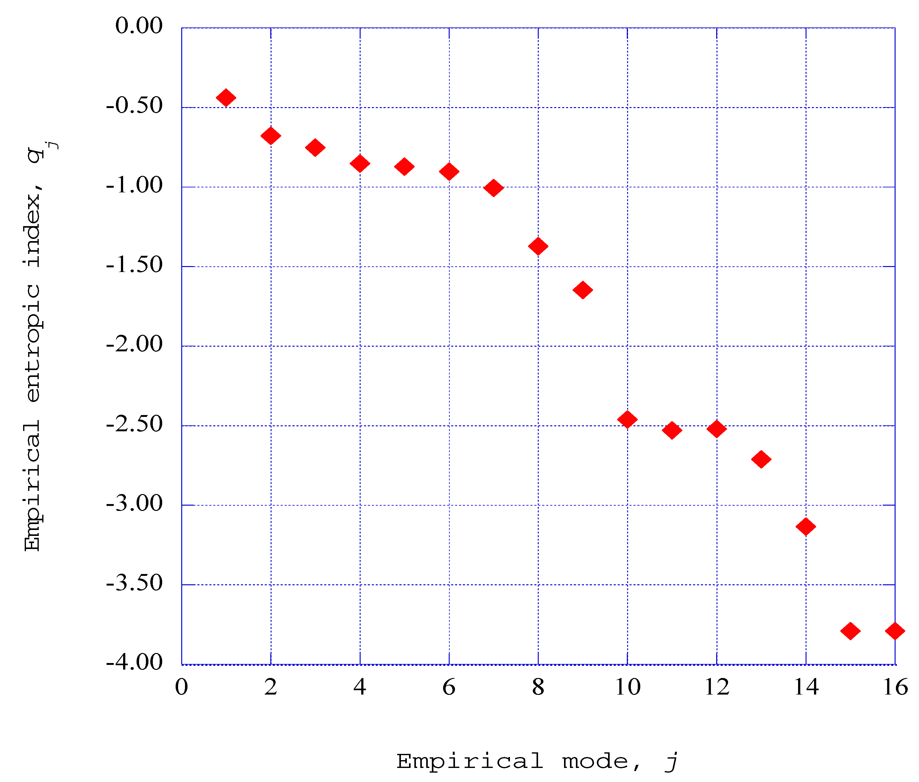
3.6. Empirical Entropic Indices for the Ordered Structures

The empirical entropies for the fluctuating spectral velocity wave component time series indicate different characteristics for the various deterministic ensembles embedded within the time series. These results indicate that the majority of the kinetic energy is contained within the first six empirical modes of the singular value decompositions, with relatively low empirical entropy. The following three empirical modes indicate a transition into deterministic ordered structures. These structures have been classified as coherent [19] with well-defined structural boundaries. We wish to find a way to follow these structures through the process of transition from ordered structures into equilibrium thermodynamic states. For this, we turn to the concept of the Tsallis entropic format (Tsallis [21]).

The Tsallis entropic format is applicable to a variety of microscopic and macroscopic sub-systems. We are working with a collection of statistical sub-systems spread over a limited number of empirical modes, j. Note that this is not a sequence over time, but is a sequence in phase space (Attard (pp. 409–412, [6])). The empirical entropy, Semp_j is introduced to describe the entropy of an ordered structure described by the empirical eigenvalue, λ_j, for the singular value decomposition empirical mode, j. Hence, we simply adopt, in an ad hoc fashion, an expression from which we may extract an empirical entropic index, q_j, from the empirical entropy, Semp_j. This expression may be written as [2]:

$$Sem{p}_j=-\text{ln}({\lambda }_j)=\frac{1-{({\lambda }_j)}^{q_j}}{(q_j-1)}$$

(5)

This expression includes the effects of the nonlinear, non-equilibrium nature of the ordered structures we are following. It has the format for an entropic index; hence, we simply call q_j the empirical entropic index or simply entropic index.

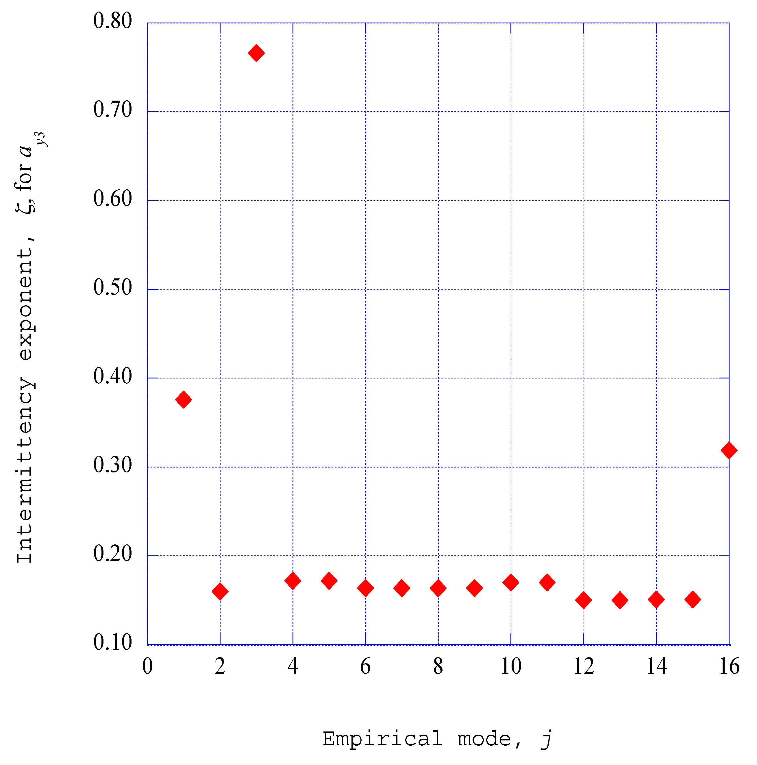
3.7. Empirical Intermittency Exponents for the Ordered Structures

In this section, we introduce a speculative method to connect the deterministic results for the entropic indices with the final phase of the dissipation of fluctuating kinetic energy into thermodynamic internal energy. We explore this computational connection through the concept of intermittency exponents and a relaxation process into the final thermodynamic entropy state.

The deterministic ordered structures discussed in previous sections are of a macroscopic nature embedded within the nonlinear time series solutions of the nonlinear equations for the fluctuating spectral velocity wave field. Singular value decomposition of the time series solutions provides empirical entropies for these deterministic structures. The empirical entropic indices of the Tsallis form extracted from the empirical entropies using Equation (5) have been used to obtain the intermittency exponents for the ordered structures. We heuristically apply a relationship, found by Arimitsu and Arimitsu [22], connecting the entropic index of Tsallis to the intermittency exponent, ζ_j. This intermittency exponent describes the fraction of fluctuating kinetic energy within the deterministic ordered structure that is dissipated into thermodynamic internal energy [2].

3.8. Kinetic Energy Available for Dissipation

The local mean flow kinetic energy, u²/2, at the normalized vertical distance, η = 3.00 from the horizontal surface, is considered as the source of kinetic energy to be dissipated through the spiral structures. This available kinetic energy is distributed over the stream wise component, the normal component and the span wise component. The fraction of kinetic energy in the stream wise velocity component is denoted as κ_x, the fraction of kinetic energy in the normal velocity component is denoted as κ_y and the fraction in the span wise velocity component denoted as κ_z. The fraction of dissipation kinetic energy within each empirical mode of the power spectral energy distribution is denoted as ξ_j. Then the total rate of dissipation of the available fluctuating kinetic energy for the stream wise, normal and span wise velocity components is the summation, over the empirical modes, j, of the product of the kinetic energy fraction of each mode times the intermittency exponent for that mode, ζ_j [5].

We have extracted corresponding empirical intermittency exponents from these entropic indices for each velocity component over the range of empirical modes. Thus, we have calculated the input energy source for the deterministic spiral structures, the fraction of the fluctuation kinetic energy available in each of the empirical modes within the deterministic ordered structures, and the fraction of the energy in each of the empirical modes that dissipates into background thermal energy, thus increasing the thermodynamic entropy.

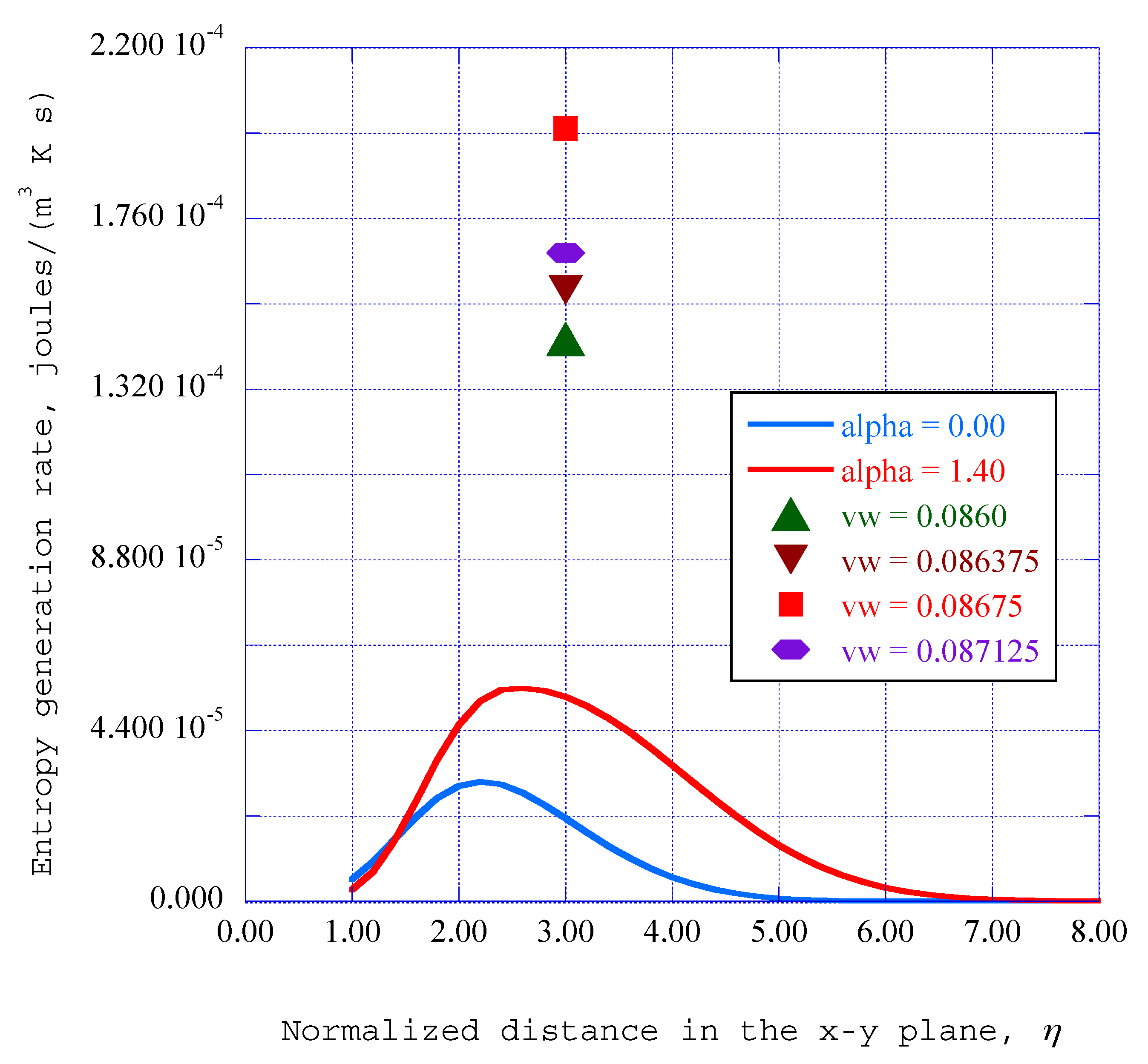
3.9. Entropy Generation Rates through the Ordered Structures

The equation for the entropy generation rate in an internal relaxation process is provided by the Gibbs equation from thermodynamics (de Groot and Mazur [23]) as:

$$\frac{\partial s}{\partial t}=-J(x)\frac{\partial \mu (x)}{\partial x}$$

(6)

In this expression, s is the entropy per unit mass, μ is the mechanical potential for the transport of the ordered structures in an external context and J(x) is the net source of the dissipation rates for the ordered kinetic energy available for dissipation.

To compute the entropy generation through the dissipation of the ordered structures, it is necessary to associate the fraction of dissipation energy in each mode of the power spectral density, ξ_j with the corresponding intermittency exponent for the singular value decomposition mode, ζ_j. This association comes about through the Wiener–Khintchine theorem (pp. 19–21, [6], and references cited therein). As shown in Figure 2, both the power spectral density and the autocorrelation function of the singular value decomposition computation process the same non-linear time series solution of the spectral velocity wave component computations. According to the Weiner–Khintchine theorem, both quantities contain the same spectral information as contained in the original non-linear time series solution. We therefore associate the peaks of the power spectral density with the corresponding intermittency exponents from the singular value decomposition.

We consider the dissipation of the ordered structures into background thermal energy as a two-stage process from the transition of the ordered structures into equilibrium thermodynamic states and a relaxation process of the stream wise velocity in the initial state to the final equilibrium state of the stream wise velocity over the internal distance x. At the final equilibrium state, the stream wise velocity of the dissipated structure vanishes. The local boundary layer steady state velocity may be written as u = u_ef’, where f’^’ is the derivative of the Falkner–Skan stream function f with respect to the normalized distance η. The expression for the entropy generation rate through the deterministic ordered structures may then be written as [1]:

$${\stackrel{•}{S}}_{gen}=\rho \left[\left(\frac{1}{2}\frac{u_e^2}{T}\right){\left(f^{\prime }\right)}^2\left\{{\kappa }_x{\left({\displaystyle \sum _{j=1}^{16}{\xi }_j{\zeta }_j}\right)}_x+{\kappa }_y{\left({\displaystyle \sum _{j=1}^{16}{\xi }_j{\zeta }_j}\right)}_y+{\kappa }_z{\left({\displaystyle \sum _{j=1}^{16}{\xi }_j{\zeta }_j}\right)}_z\right\}\left(\frac{u_e}{x}\right)\right].$$

(7)

In this expression, ρ is the density of the working substance, in this case air at the given pressure and temperature. Figure 2 presents a flow chart for the computational components as discussed in this section.

Figure 2. This flow chart summarizes the overall computational procedure used to compute the entropy generation through deterministic ordered structures.

Figure 2. This flow chart summarizes the overall computational procedure used to compute the entropy generation through deterministic ordered structures.

For a comparison of the entropy generation rates from this expression, the entropy generation rates within a turbulent boundary layer are computed for each given stream wise location, first with zero pressure gradient and then with an adverse pressure gradient. Following Truitt [24] and Bejan [25], the expression for the entropy generation rates in a turbulent boundary layer may be written as:

$${\stackrel{•}{S}}_{turb}=\rho \frac{(\upsilon +{\epsilon }_m)}{T}{(\frac{\partial u}{\partial y})}^2$$

(8)

In this expression, ε_m is defined as the “eddy viscosity”, (Cebeci and Bradshaw, pp. 153–159, [8]), having the dimensions of (viscosity)/(density) which relates the turbulent shear stress to the stream wise boundary layer velocity gradient.

For our comparison, we consider a turbulent boundary layer with a zero pressure gradient and a turbulent boundary layer with an adverse pressure gradient. The adverse pressure gradient is included in the boundary-layer computations with the term (Cebeci and Bradshaw, pp. 268–269, [8]):

$$P2=-\alpha \frac{x}{u_e}$$

(9)

In this expression, P2 is the computed pressure gradient parameter and α is a pressure gradient coefficient set equal to 1.40. This value for the adverse pressure gradient applied to the turbulent boundary layer yields a surface skin friction coefficient of approximately zero value.

The computation of the turbulent boundary layer begins at the initial stream wise station x = 0.02 with transition enforced at that location. Hence, the turbulent boundary layer for our calculations at the stream wise location x = 0.12 is much smaller than a naturally occurring transition further along the stream wise direction. Ghasemisahebi [26] presents the results of a study of the entropy generation process in the bypass transition region of a flat plate boundary layer under strong levels of free stream turbulence and stream wise pressure gradients, providing insight into the entropy generation processes near the flat plate surface.

4. Results

Computational Results for the Receiver Stations

Figure 3 presents the fluctuating stream wise spectral velocity wave component, a_x3, for the third receiver station, as a function of the time step number over the total time range of the integration process. Figure 4 shows the corresponding phase diagram for a_z3-a_y3, where a_y3 is the normal spectral velocity wave component and a_z3 is the span wise spectral velocity wave component, again at the third receiver station.

Figure 3. The stream wise spectral velocity wave component, a_x3, is shown as a function of time step number at the third receiver station x = 0.12 with w_e = 0.086375.

Figure 3. The stream wise spectral velocity wave component, a_x3, is shown as a function of time step number at the third receiver station x = 0.12 with w_e = 0.086375.

Figure 4. The phase diagram of the span wise and normal spectral velocity components, a_z3-a_y3, is shown for the third receiver station x = 0.12 with w_e = 0.086375.

Figure 4. The phase diagram of the span wise and normal spectral velocity components, a_z3-a_y3, is shown for the third receiver station x = 0.12 with w_e = 0.086375.

The resulting power spectral density results for the normal spectral velocity wave component, a_y3 at the third receiver station at x = 0.12, are presented in Figure 5. Very fine grids are required to extract these results. We have assigned empirical mode numbers to these peaks, starting with mode j = 1 representing the highest peak in the distribution, continuing to mode j = 16, representing the corresponding lowest peak among the sixteen peaks.

Figure 5. The power spectral density for the normal spectral velocity component is shown for the third receiver station x = 0.12 with w_e = 0.086375.

Figure 5. The power spectral density for the normal spectral velocity component is shown for the third receiver station x = 0.12 with w_e = 0.086375.

The kinetic energy in each spectral mode available for final dissipation into equilibrium internal energy is computed for each of these spectral peaks. The empirical entropy for each of the structures indicated by the spectral peaks is found from the singular value decomposition process applied to the given time series data segment. The connecting parameter, the empirical entropic index, is then extracted from the resulting value of the empirical entropy.

The expression for the empirical entropic index, q_j is given in Equation (5). We have used this expression to extract the empirical entropic index from the empirical entropy for the third receiver station at x = 0.12. Figure 6 shows the entropic index for the normal spectral velocity wave component at this station as a function of the empirical mode j, for a mass injection velocity of w_e = 0.08375. The first six modes indicate a fairly smooth region with entropic indices slightly below zero, indicating that these structures are only of a slightly dissipative nature. Modes seven through eleven indicate a significant transition region into non-equilibrium ordered structures. Modes twelve through sixteen indicate the possible further transition into further ordered states. We should note at this point that these indices are not in a sequence in time, but exist as a collection of modes within the fluctuating time series solution (Attard, pp. 409–414, [6]).

Figure 6. The empirical entropic index for the normal spectral velocity component, a_y3, is shown as a function of the empirical mode, j for the third receiver station at x = 0.12 with the surface mass injection velocity w_e = 0.08375.

Figure 6. The empirical entropic index for the normal spectral velocity component, a_y3, is shown as a function of the empirical mode, j for the third receiver station at x = 0.12 with the surface mass injection velocity w_e = 0.08375.

Glandsdorff and Prigogine [27] find that for the general evolution criterion for non-equilibrium dissipative processes, dSemp_j/dt < 0. When the Tsallis entropic index is negative, Mariz [28] found that the empirical entropy change is also negative, dSemp_j/dt < 0. The results presented in Figure 6 indicate that significant deterministic structures exist within the specified time frame of the nonlinear time series solution. These regions may therefore be classified as ordered, dissipative structures. Therefore, the significant negative nature for the extracted empirical entropic indices at the third receiver station at x = 0.12 is in agreement with both the Prigogine criterion and the Mariz results for the Tsallis entropic index. The ad hoc introduction of an empirical entropy index thus provides a representation of the nonlinear, non-equilibrium ordered structures in a significant way.

Given the absolute value of the empirical entropic index, q_j, the intermittency exponent, ζ_j for the mode, j, is extracted from the expression given by Arimitsu and Arimitsu [22] by the use of Brent’s method (pp. 397–405, [18]). The intermittency exponent for the normal spectral velocity component, a_y3, at the third receiver station at x = 0.12 for the surface injection velocity w_e = 0.086375 is shown in Figure 7 as a function of the empirical mode, j.

Figure 7. The intermittency exponent for the normal spectral velocity component, a_y3, is shown for the third receiver station at x = 0.12 with w_e = 0.086375 as a function of empirical mode, j.

Figure 7. The intermittency exponent for the normal spectral velocity component, a_y3, is shown for the third receiver station at x = 0.12 with w_e = 0.086375 as a function of empirical mode, j.

We consider the entropy generation rate to be a phase transition of the dissipation of the ordered structure into background thermal energy and a relaxation process of the global mechanical transport process of the stream wise velocity, u_e over the distance x. At the final equilibrium state, the stream wise velocity of the dissipated structure vanishes. The entropy generation rates through the deterministic ordered structures may then be determined from Equation (7) [1].

Equation (7) has the form found experimentally by Mazellier and Vassilicos [29] for the dissipation of turbulence energy in fractal grid-generated wind tunnel flows. The general form is that the dissipation of the ordered structure energy is proportional to the quadratic form of the velocity and that the mechanical turnover rate is a function of the global parameters u_e/x.

The entropy generation rates as a function of the stream wise stations are shown in Figure 8, with the four values of surface injection velocities as the imposed crosswind parameters. Note that each crosswind velocity is constant in the stream wise direction.

Figure 8 shows only the entropy generation rates for the receiver stations, and not the rate for the transmitter station. It is interesting to note that the rate of entropy generation for the second receiver station is considerably lower than the rates for the other receiver stations. Also, only the nonlinear solutions for two of the injection velocities contribute to the entropy generation at the first and second receiver stations. These results indicate that the deterministic spiral structures at the first and second receiver stations are primarily smooth functions, with much lower levels of fluctuation energy than for the following receiver stations.

Figure 8. The entropy generation rates for the ordered structures are shown for various mass injection velocities at several stream wise stations.

Figure 8. The entropy generation rates for the ordered structures are shown for various mass injection velocities at several stream wise stations.

The abrupt increases in the entropy generation rates at the third receiver station indicate a burst of fluctuation energy in the nonlinear time series solutions for the spectral velocity wave components at this station. Note that the largest increase occurs for the surface injection velocity of w_e = 0.08675, and not for the highest injection velocity. This result implies that there is an optimum surface injection velocity for the creation of fluctuations within the deterministic spiral structures. The entropy generation rates then decline over the remaining stream wise receiver stations.

For a comparison of these values for the entropy generation rates, the entropy generation rates within a turbulent boundary layer are computed for each given stream wise location. Applying the Falkner–Skan transformation in the differentiation with respect to y in Equation (8) and the definition of the term:

$${\epsilon }_m^{÷}=\frac{{\epsilon }_m}{\nu },$$

(10)

the entropy generation rates across the turbulent boundary layer may be written from Equation (8) as:

$${\stackrel{•}{S}}_{turb}=\rho \left(\frac{1}{2}\frac{u_e^2}{T}\right){\left(f^{\prime }\right)}^2(1+{\epsilon }_m^{+}){(f^{″})}^2(\frac{u_e}{x}).$$

(11)

The computation of the turbulent boundary layer begins at the initial stream wise station x = 0.02 with transition enforced at that location. Hence, the turbulent boundary layer for our calculations at the stream wise location x = 0.12 is much smaller than for a naturally occurring transition further along the stream wise direction. The distribution of the entropy generation rates across the turbulent boundary layer for zero pressure gradient and for the adverse pressure gradient for which the skin friction coefficient approaches zero are shown in Figure 9.

Figure 9. The entropy generation rates for the deterministic ordered structures at x = 0.12 for various injection velocities are compared with the entropy generation rates across turbulent boundary layers with and without an applied adverse pressure gradient as a function of the normalized distance from the horizontal surface.

Figure 9. The entropy generation rates for the deterministic ordered structures at x = 0.12 for various injection velocities are compared with the entropy generation rates across turbulent boundary layers with and without an applied adverse pressure gradient as a function of the normalized distance from the horizontal surface.

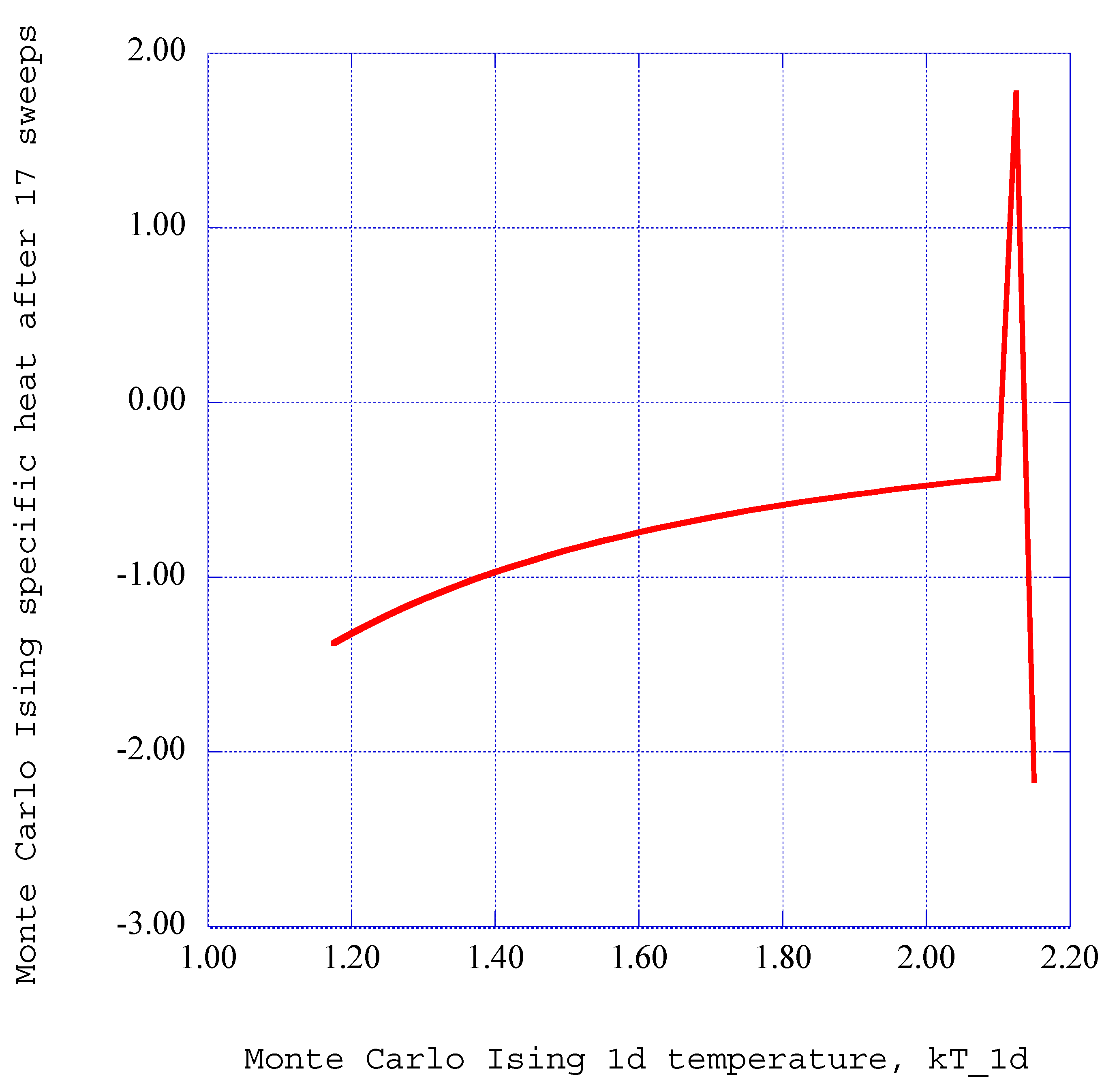
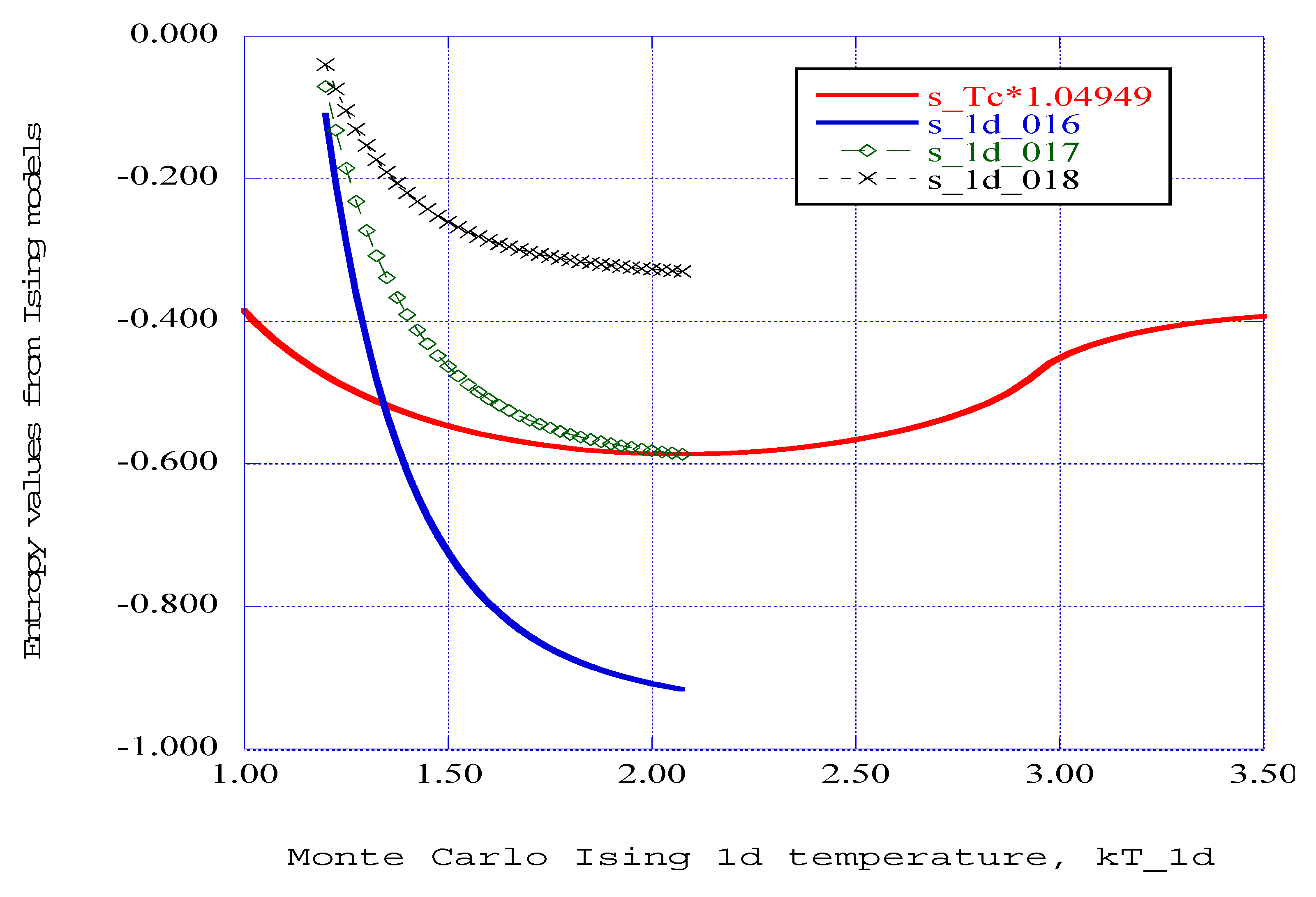
5. On the Transition of Non-Equilibrium Ordered Structures into Equilibrium Thermodynamic States

The negative values that we calculate for the empirical entropic indices provide an opportunity for us to examine the transition of non-equilibrium ordered structures into equilibrium thermodynamic states. According to Mariz [29], a negative value for the Tsallis entropic index indicates that the entropy change is also negative. For a negative entropy change, the general evolution criterion given by Glandsdorff and Prigogine [28] indicates that such systems are non-equilibrium dissipative structures, which we have classified as non-equilibrium ordered structures. Hatsopolos and Keenan [30] characterize these systems as having negative absolute temperatures, with higher driving potentials for dissipation into the reservoir equilibrium thermodynamic states. Anderson and Lim [31] discuss the concept of negative temperature states in the context of vortex filaments in equilibrium. The discussion presented in [31] has direct application to the modeling of our non-equilibrium ordered states.

The Ising model of a magnet (Huang [32]) represents the transition of an ordered system into a disordered system. The Ising model considers the transition of a selection of ordered sites on a lattice structure into a resulting collection of disordered sites. This model has been studied extensively and both exact and Monte Carlo solutions have been obtained (Landau and Binder [33]). It is interesting that exact and Monte Carlo studies of the critical antiferromagnetic material behavior indicate the presence of a singularity or critical spike in the value of the specific heat of the material (pp. 15–18, [33]) as the material passes through a critical temperature. We wish to apply this model to a consideration of the mechanism of the transition of our non-equilibrium ordered structures into equilibrium thermodynamic states.

Exact solutions of the two-dimensional Ising model have been presented in Huang [32] and Baxter [34]. For the two-dimensional Onsager solution near the critical temperature, T = T_c, Huang (pp. 370–373, [32]) presents an approximate expression for the specific heat of the material as a function of the normalized temperature, kT, as the temperature is varied through the critical point. Here, k is Boltzmann’s constant and T is the absolute temperature. The behavior of the Ising model specific heat Cv/k as a function of the temperature is shown in Figure 10.

Figure 10. The specific heat of the two-dimensional Ising model is shown as a function of the Ising temperature, kT.

Figure 10. The specific heat of the two-dimensional Ising model is shown as a function of the Ising temperature, kT.

The corresponding entropy for the Ising model is found by integrating the specific heat divided by the temperature over the range of temperature. Simpson’s rule is used to obtain the Ising entropy over the temperature range near the critical temperature. The dimensionless entropy results are shown in Figure 11 as a function of the Ising temperature, kT.

Figure 11. The entropy of the two-dimensional Ising model obtained from the specific heat values for the model is shown as a function of the Ising temperature, kT.

Figure 11. The entropy of the two-dimensional Ising model obtained from the specific heat values for the model is shown as a function of the Ising temperature, kT.

The results presented in these two figures provide significant insight into the mechanisms at work in the transition of our ordered structures into equilibrium thermodynamic states. Starting at the very left of the specific heat curve in Figure 9, the value of the specific heat is negative. This corresponds to the ordered structures predicted in our computations. As the sub-system temperature increases, the specific heat crosses the zero line and becomes positive. The corresponding behavior of the entropy of the ordered sub-system shown in Figure 10 indicates that the entropy appears at a high value in the ordered structure and decreases as the temperature increases, reaching a minimum as the specific heat of the material reaches and crosses the zero line. Then the entropy increases to a maximum when the specific heat again crosses the zero line, at which point the entropy begins to decrease. We consider the point of maximum entropy on the right-hand side of the singularity as the equilibrium thermodynamic state of the reservoir, and thus the final equilibrium thermodynamic state of our ordered structure. We thus fulfill the non-equilibrium criteria discussed by Attard (pp. 47–48, [6]) and Tsallis (pp. 90–98, pp. 156–158, [21]).

We have applied a Monte Carlo simulation analysis to a one-dimensional ten-site Ising lattice to get a better understanding of the transition process of our non-equilibrium ordered structures into the equilibrium thermodynamic state. The computer program listing presented by Landau and Binder (pp. 358–363, [33]) is used to calculate the specific heat of the lattice as a function of the lattice temperature for a selected number of lattice sweeps. Figure 12 shows the specific heat of the lattice after seventeen computational sweeps through the lattice. The lattice temperature range is from 1.175 to 2.150 and includes both negative and positive values for the specific heat. The corresponding entropy values are obtained by Simpson integration of the ratio of specific heat to absolute temperature over the temperature range. These results are shown in Figure 13. For comparison, also shown in Figure 13 is the entropy obtained from the approximate specific heat expression for the exact Onsager solution of the two-dimensional Ising model given by Huang (pp. 370–373, [32]).

Figure 12. The specific heat of a one-dimensional Ising model using a Monte Carlo simulation is shown as a function of the Ising 1d temperature, kT.

Figure 12. The specific heat of a one-dimensional Ising model using a Monte Carlo simulation is shown as a function of the Ising 1d temperature, kT.

Figure 13. Comparison of a one-dimensional Monte Carlo simulation and a two-dimensional approximate solution for the entropy of the Ising model is shown as a function of the Ising temperature, kT.

Figure 13. Comparison of a one-dimensional Monte Carlo simulation and a two-dimensional approximate solution for the entropy of the Ising model is shown as a function of the Ising temperature, kT.

The specific heats for the Ising model shown in Figure 10 and Figure 12 indicate negative values for low values of the Ising temperature, kT. We assume that the values of the specific heats at the low temperatures are the specific heats for the ordered structures that we have been following through the computational process. To interpret the implications of a negative value for the specific heat, we note that the specific heat is a thermodynamic state function for a given ordered structure. If an increment of energy is added to the structure, a negative specific heat indicates that energy in the ordered kinetic energy of the structure is increased, while the energy of the disordered portion of the structure is decreased. This is in agreement with the entropy, which indicates a corresponding decrease in value as the increment of energy is added.

As the Ising temperature of the sub-system is increased, a smaller portion of the increment of added energy resides in the ordered portion of the sub-system, while the disordered portion increases in temperature. The rate of decrease in the entropy therefore decreases, until the entropy reaches a minimum. At this point, the specific heat of the sub-system is zero, and a further increase in the sub-system temperature indicates a positive value for the specific heat.

When the entropy reaches the minimum, the sub-system undergoes a spontaneous phase transition into the equilibrium thermodynamic state. In this process, the entropy increases to its maximum value, equal to the reservoir equilibrium entropy.

The results from the applications of various simulations of the one and two-dimensional Ising models indicate that non-equilibrium Monte Carlo simulation techniques may provide accurate analysis of our ordered structure transition into the reservoir equilibrium thermodynamic state. Monte Carlo simulation methods are well established in the physics community, with recent developments provided by Attard (pp. 409–435, [6]), Newman and Barkema [35], Lim and Nebus [36], and Liang, Liu, and Carroll [37].

6. Discussion

It has previously been found that a crosswind velocity in a corner boundary layer flow could trigger instabilities in the three-dimensional laminar boundary layer along the horizontal surface [1]. This crosswind velocity had been attributed to the developing boundary layer along the sidewall surface. For a stream wise velocity of 1.0, it was found that a crosswind velocity above 0.0830 is necessary to initiate instabilities within the laminar boundary layer environment. However, the magnitude of the crosswind velocity due to sidewall boundary layer development is insufficient to initiate laminar boundary layer instabilities. Crosswind velocities of sufficient magnitude to initiate instabilities require the injection of an additional flow along the sidewall in the z-direction of the horizontal surface of the flow configuration. This flow into the boundary layer provides the development of an additional boundary layer profile in the z-y plane along the horizontal surface, thus providing a three-dimensional orthogonal boundary layer environment.

Application of coupled, nonlinear modified Lorenz equations in the spectral plane of the flow environment indicates the generation of deterministic spiral structures in the three-dimensional environment. Fluctuating spectral velocity components are found within the three spectral velocity component time-series solutions for these equations. Statistical processing of the solutions indicates the presence of ordered structures embedded within the fluctuating time-series environment. The transition of these ordered structures into equilibrium thermodynamic states yields the entropy generation rates for the overall process.

For the results reported here, the effects of four sidewall injection velocity values are evaluated, w_e = 0.0860, 0.086375, 0.08750, 0.87125, at six stream wise stations along the x-axis. These values are well above the threshold value for the initiation of instabilities. However, it is surprising that significant variation in the magnitude of the ordered structures occurs over a very narrow range of injection velocities.

Each value of injection velocity is applied uniformly through the sidewall along the stream wise boundary layer. To include the synchronization properties of the modified Lorenz equations, the first station is labeled as the transmitter station with the subsequent five stations as receiver stations. Computational results for the transmitter station, and each following receiver station indicate significant deterministic spiral structure production for each of the stations. The intensity of the power spectral densities within these deterministic structures varies from station to station, indicating the triggering of significantly different structures for each station. It should also be noted that not all of the spectral velocity component time series solutions exhibit fluctuating content. Only the contributions from fluctuating time series are included in the computation of the respective rates of entropy generation.

For example, only the fluctuating velocity components for the two lowest injection velocities contribute to the entropy generation at the first receiver station. At the second receiver station, only fluctuations from the lowest injection velocity and the highest injection velocity contribute to the entropy generation, yielding a significantly decreased rate of entropy generation.

At the third receiver station, the four injection velocities indicate high rates of entropy production, with the third highest injection velocity producing a spike or burst of entropy generation. The following two receiver stations indicate a more systematic decrease in entropy generation rate, thus indicating a more uniform production of deterministic ordered structures within the fluctuating ordered regions. These results imply that an optimum injection velocity exists for the generation of dissipative velocity fluctuations.

To gain a perspective on the magnitude of the predicted rates of entropy generation through the transition of ordered structures, a comparison is made with the rate of entropy generation in turbulent boundary layers with a zero pressure gradient and an adverse pressure gradient. For a turbulent boundary layer initiated at the leading edge of the horizontal surface, the entropy generated by a turbulent boundary layer with zero pressure gradient is nearly an order of magnitude smaller than the rate of entropy generation through the ordered structures with sidewall surface mass injection.

For a turbulent boundary layer with an adverse pressure gradient sufficient to bring the surface skin friction to zero, the rate of entropy generated by the turbulent boundary layer is nearly three times smaller than the rate of entropy generation through the ordered structures.

Finally, observations of the characteristics of the transition of the Ising model from ordered structures into equilibrium thermodynamic states may provide a method for understanding the physics of the transition of our non-equilibrium ordered structures into final reservoir equilibrium thermodynamic states.

7. Conclusions

An innovative computational procedure is discussed that predicts time-dependent instabilities and deterministic ordered structures in three-dimensional steady-state laminar boundary-layer flows. The three-dimensional flow configuration considered in this study is a corner flow with sidewall surface mass injection into a horizontal laminar boundary-layer flow. The three equations for the velocity fluctuations in the physical plane are transformed into six equations in the spectral plane. These six equations include three linear first-order differential equations for the spectral wave numbers and three nonlinear coupled first-order differential equations for the spectral velocity wave components. These three nonlinear spectral velocity equations are arranged into a Lorenz-format system of equations and incorporated in the overall computational system. Computational results from these spectral Lorenz-form equations indicate that sidewall surface mass injection, for injection velocities above a critical value, will initiate strong deterministic instabilities in the three-dimensional horizontal surface boundary layer flow environment. These instabilities take the form of deterministic spiral structures with embedded spectral velocity component fluctuations. The power spectral density of the fluctuations indicates regions of ordered structures within the nonlinear time series solutions of the governing equations. For a narrow range of injection velocities above the critical value, computation of the entropy generation rates at six x-axis stations indicates a significant level of entropy generation, with a burst of entropy generation occurring at the fourth of the x-axis stations. This burst occurs for the higher range of surface injection velocities. It is shown that there exists an “optimum” injection velocity for which the entropy generation is a maximum. If the objective of the flow device under design is to optimize a surface heat transfer rate, this information is directly applicable. If the objective of the device under design is to rapidly mix an injected fuel with the flowing oxidizer, such mixing will take place within the dissipation of the ordered structures into the equilibrium thermodynamic state of the reservoir system. We have noted that the range of kinematic viscosities is quite limited for the prediction of instabilities in the three-dimensional flow configurations we have considered. At this point, the computational procedure is therefore applicable to only a selected few thermodynamic flow systems. Thus, much work needs to be done to clarify the range of kinematic viscosities over which this innovative computational procedure may be applied. Finally, the computational results for the various processes occurring in the generation, transition and dissipation of the ordered structures into thermodynamic entropy are placed in a corresponding non-equilibrium thermodynamics context.

References

1. Isaacson, L.K. Entropy Generation through Deterministic Spiral Structures in a Corner Boundary-Layer Flow. Entropy 2015, 17, 5304–5332. [Google Scholar] [CrossRef]
2. Isaacson, L.K. Ordered Regions within a Nonlinear Time Series Solution of a Lorenz Form of the Townsend Equations for a Boundary-Layer Flow. Entropy 2013, 15, 53–79. [Google Scholar] [CrossRef]
3. Isaacson, L.K. Spectral Entropy, Empirical Entropy and Empirical Exergy for Deterministic Boundary-Layer Structures. Entropy 2013, 15, 4134–4158. [Google Scholar] [CrossRef]
4. Isaacson, L.K. Spectral Entropy in a Boundary Layer Flow. Entropy 2011, 13, 1555–1583. [Google Scholar] [CrossRef]
5. Isaacson, L.K. Entropy Generation through a Deterministic Boundary-Layer Structure in Warm Dense Plasma. Entropy 2014, 16, 6006–6032. [Google Scholar] [CrossRef]
6. Attard, P. Non-Equilibrium Thermodynamics and Statistical Mechanics: Foundation and Applications; Oxford University Press: Oxford, UK, 2012. [Google Scholar]
7. Hansen, A.G. Similarity Analyses of Boundary Value Problems in Engineering; Prentice-Hall, Inc.: Englewood Cliffs, NJ, USA, 1964; pp. 86–92. [Google Scholar]
8. Cebeci, T.; Bradshaw, P. Momentum Transfer in Boundary Layers; Hemisphere: Washington, DC, USA, 1977; pp. 319–321. [Google Scholar]
9. Cebeci, T.; Cousteix, J. Modeling and Computation of Boundary-Layer Flows; Horizons Publishing Inc.: Long Beach, CA, USA, 2005. [Google Scholar]
10. Townsend, A.A. The Structure of Turbulent Shear Flow, 2nd ed.; Cambridge University Press: Cambridge, UK, 1976. [Google Scholar]
11. Isaacson, L.K. Transitional Intermittency Exponents through Deterministic Boundary-Layer Structures and Empirical Entropic Indices. Entropy 2014, 16, 2729–2755. [Google Scholar] [CrossRef]
12. Mathieu, J.; Scott, J. An Introduction to Turbulent Flow; Cambridge University Press: New York, NY, USA, 2000; pp. 251–261. [Google Scholar]
13. Manneville, P. Dissipative Structures and Weak Turbulence; Academic Press, Inc.: San Diego, CA, USA, 1990. [Google Scholar]
14. Pecora, L.M.; Carroll, T.L. Synchronization in chaotic systems. In Controlling Chaos: Theoretical and Practical Methods in Nonlinear Dynamics; Kapitaniak, T., Ed.; Academic Press Inc.: San Diego, CA, USA, 1996; pp. 142–145. [Google Scholar]
15. Pérez, G.; Cerdeiral, H.A. Extracting messages masked by chaos. In Controlling Chaos: Theoretical and Practical Methods in Nonlinear Dynamics; Kapitaniak, T., Ed.; Academic Press Inc.: San Diego, CA, USA, 1996; pp. 157–160. [Google Scholar]
16. Cuomo, K.M.; Oppenheim, A.V. Circuit implementation of synchronized chaos with applications to communications. In Controlling Chaos: Theoretical and Practical Methods in Nonlinear Dynamics; Kapitaniak, T., Ed.; Academic Press Inc.: San Diego, CA, USA, 1996; pp. 153–156. [Google Scholar]
17. Chen, C.H. Digital Waveform Processing and Recognition; CRC Press, Inc.: Boca Raton, FL, USA, 1982; pp. 131–158. [Google Scholar]
18. Press, W.H.; Teukolsky, S.A.; Vetterling, W.T.; Flannery, B.P. Numerical Recipes in C: The Art of Scientific Computing, 2nd ed.; Cambridge University Press: Cambridge, UK, 1992. [Google Scholar]
19. Holmes, P.; Lumley, J.L.; Berkooz, G.; Rowley, C.W. Turbulence, Coherent Structures, Dynamical Stations and Symmetry, 2nd ed.; Cambridge University Press: Cambridge, UK, 2012. [Google Scholar]
20. Rissanen, J. Information and Complexity in Statistical Modeling; Springer: New York, NY, USA, 2007. [Google Scholar]
21. Tsallis, C. Introduction to Nonextensive Statistical Mechanics; Springer: New York, NY, USA, 2009; pp. 37–43. [Google Scholar]
22. Arimitsu, T.; Arimitsu, N. Analysis of fully developed turbulence in terms of Tsallis statistics. Phys. Rev. E 2000, 61, 3237–3240. [Google Scholar] [CrossRef] [Green Version]
23. De Groot, S.R.; Mazur, P. Non-Equilibrium Thermodynamics; North-Holland Pub. Co.: Amsterdam, The Netherlands, 1962. [Google Scholar]
24. Truitt, R.W. Fundamentals of Aerodynamic Heating; The Ronald Press Company: New York, NY, USA, 1960. [Google Scholar]
25. Bejan, A. Entropy Generation Minimization; CRC Press LLC: Boca Raton, FL, USA, 1996. [Google Scholar]
26. Ghasemisahebi, E. Entropy Generation in Transitional Boundary Layers; LAP LAMBERT Academic Publishing: Saarbrücken, Germany, 2013. [Google Scholar]
27. Glansdorff, P.; Prigogine, I. Thermodynamic Theory of Structure, Stability and Fluctuations; John Wiley & Sons Ltd.: London, UK, 1971. [Google Scholar]
28. Mariz, A.M. On the irreversible nature of the Tsallis and Renyi entropies. Phys. Lett. A 1992, 165, 409–411. [Google Scholar] [CrossRef]
29. Mazellier, N.; Vassilicos, J.C. Turbulence without Richardson-Kolmogorov cascade. Phys. Fluids 2010, 22, 075101. [Google Scholar] [CrossRef]
30. Hatsopoulos, G.N.; Keenan, J.H. Principles of General Thermodynamics; John Wiley & Sons, Inc.: New York, NY, USA, 1965. [Google Scholar]
31. Anderson, T.D.; Lim, C.C. Introduction to Vortex Filaments in Equilibrium; Springer Science + Business Media: New York, NY, USA, 2014. [Google Scholar]
32. Huang, K. Statistical Mechanics; John Wiley & Sons, Inc.: New York, NY, USA, 1963. [Google Scholar]
33. Landau, D.P.; Binder, K. A Guide to Monte Carlo Simulations in Statistical Physics; Cambridge University Press: Cambridge, UK, 2002. [Google Scholar]
34. Baxter, R.L. Exactly Solved Models in Statistical Mechanics; Dover Publications, Inc.: Mineola, NY, USA, 2007. [Google Scholar]
35. Newman, M.E.J.; Barkema, G.T. Monte Carlo Methods in Statistical Physics; Oxford University Press Inc.: New York, NY, USA, 2002. [Google Scholar]
36. Lim, C.; Nebus, J. Vorticity, Statistical Mechanics, and Monte Carlo Simulation; Springer Science + Business Media, LLC: New York, NY, USA, 2007. [Google Scholar]
37. Liang, F.; Liu, C.; Carroll, R.J. Advanced Markov Chain Monte Carlo Methods: Learning from Past Examples; John Wiley & Sons Ltd.: West Sussex, UK, 2010. [Google Scholar]