
Entropy Production in the Theory of Heat Conduction in Solids


1
Department of Mathematics and Physics, Roma Tre University, Via della Vasca Navale 84, 00146 Roma, Italy
2
INFN Section of Roma Tre, Department of Mathematics and Physics, Via della Vasca Navale 84, 00146 Roma, Italy
Entropy 2016, 18(3), 87; https://0-doi-org.brum.beds.ac.uk/10.3390/e18030087
Submission received: 11 January 2016
/
Revised: 13 February 2016
/
Accepted: 26 February 2016
/
Published: 8 March 2016
(This article belongs to the Special Issue Maximum versus Minimum Entropy Generation: Theoretical Developments and Applications)
Abstract
:The evolution of the entropy production in solids due to heat transfer is usually associated with the Prigogine’s minimum entropy production principle. In this paper, we propose a critical review of the results of Prigogine and some comments on the succeeding literature. We suggest a characterization of the evolution of the entropy production of the system through the generalized Fourier modes, showing that they are the only states with a time independent entropy production. The variational approach and a Lyapunov functional of the temperature, monotonically decreasing with time, are discussed. We describe the analytic properties of the entropy production as a function of time in terms of the generalized Fourier coefficients of the system. Analytical tools are used throughout the paper and numerical examples will support the statements.
1. Introduction
The minimum entropy production principle states that in the regime of linear irreversible thermodynamics, the steady state of an irreversible process is characterized by a minimum value of the rate of entropy production. It was formulated by Prigogine in 1947 [1] and successively different authors, including Prigogine himself and his coworkers, tried to generalize it and to put forth new examples and new areas of application for the principle: for example it has been employed in chemistry, biology, ecology and, obviously, in engineering sciences (see, e.g., [2] and references therein). In addition, due to these large number of applications, different statements about the principle, its validity and applicability have been given in the literature. Prigogine returned different times in the course of his life on the principle, approaching the problem from different points of view: maybe this is one of the causes of different misconceptions about the principle. Indeed one of the most frequent applications of the principle that we can find in the works of Prigogine is on the theory of heat conduction in solids. However, as it has been recently noticed [2,3,4], in this case the principle cannot be applied (we return on this point in the next sections). The question arising is then to characterize the evolution of the rate of entropy production due to heat transfer in solids.
The aim of this paper is twofold: on the one hand, we would like to clarify, once more the limits of applicability of the Prigogine minimum entropy production principle (for a critical review of this aspect of the work of Prigogine, see [2]); and, on the other hand, we wish to answer to the following questions: Does the rate of entropy production due to heat conduction in solids follows a minimum principle? If not, are there “preferred” (in a sense to be specified) thermodynamic states with respect to the production of entropy? If the linear Fourier law holds, how can we characterize the entropy production of the solid?
According to the previous plan, the paper is organized as follows: in Section 2, we analyze the minimum entropy production principle applied to the case of heat transfer in solids, starting from the considerations made by Prigogine and coworkers and after commenting on more recent papers and critical reviews. The analysis of the principle according to variational methods and a Lyapunov functional of the temperature monotonically decreasing with the evolution of the system will be discussed too. In Section 3, we illustrate the fundamental role played by the generalized Fourier modes (the eigenvectors of the Helmholtz operator times an exponential of the time) to characterize the long-time behavior of the entropy production. Further, we show that there are preferred time-dependent states having a constant entropy production: these are precisely the generalized Fourier modes. We show that these are the only states having this property. In Section 4, we consider the behavior of the entropy production as a function of time, showing, in general and in concrete cases, that the stationary state of the system does not necessarily correspond to a minimum of the entropy production. The leading term in the generalized Fourier expansion plays a major role. Numerical and analytic examples are given. Finally, in the conclusions, we comment on our findings, acknowledge the conditions of applicability and validity of the minimum entropy production, emphasize those situations giving misleading or erroneous results and provide a systematic view of our results.
2. The Minimum Entropy Production Principle and the Heat Conduction in Solids
In this section, we review the minimum entropy production principle in the theory of heat conduction in solids as formulated by Glansdorff and Prigogine [5]. It is not our intention to dispute the minimum entropy production principle from a general point of view: it is well known that, provided certain specific assumptions are satisfied, the principle is undoubtedly valid (see, e.g., [2] and references therein). However, Prigogine himself considered the case of thermal conduction in solids one of the simplest application of the general principle (see, e.g., [5,6,7]) and used different approaches (see [5,6,7,8]) to conclude that the entropy production in diffusive processes, if the temperature is fixed at the system boundary, tends to decrease with time and reaches a minimum in a final steady state. Thus, it is this statement, or the application of the general principle to the case of heat conduction in solids, that we discuss. Let us look at the proof given by Glansdorff and Prigogine in [5] (see also [9]). The postulates of the authors are:
where is a constant (postulate b). The entropy production can be written as [1,2,3,4,5,6,7]
and the time derivative of the entropy production, using the fact that is a constant from postulate (b), is
By integrating by parts one gets:
The first integral, using the divergence theorem, becomes:
and it is zero (postulate d). The other integral gives:
At this point, the author’s uses the energy conservation; that is, ( is the density of the homogeneous material and its specific heat, assumed to be constant.). Since is given by Equation (1), one gets:
which is negative. This means that is always negative; that is, the entropy production is a decreasing function of time and will reach a minimum in the final steady state.
- (a)
- The relations between the generalized forces and fluxes are linear. In this case it means that the heat flux is proportional to the gradient of the inverse of temperature, i.e., , where is the phenomenological coefficient.
- (b)
- The phenomenological coefficients are constants.
- (c)
- The Onsager reciprocity relation holds (trivial in this case, since we have just one phenomenological coefficient).
- (d)
- The temperature on the boundaries of the solid is constant in time.
The problem in this derivation is the energy conservation law. Indeed, according to Equation (1), it reads:
Thus, to arrive at the result (Equation (7)), it has been assumed that the evolution of the temperature is described by Equation (8) instead of the usual Fourier linear equation ( is the thermal conductivity of the solid):
Glansdorff and Prigogine were aware of this difficulty, or at least were unsatisfied with their derivation, since in successive works they tried to circumvent the problem by looking at some different approaches. For example in [8], they start from the linear Fourier Equation (9) by assuming that the phenomenological coefficient depends on the temperature as . But then they find the steady state by minimizing a new quantity, not having the dimensionality of an entropy production (see also [2]), obtained by introducing a weighted expression for the thermodynamic forces; that is, assuming that the thermodynamic force, in this case, is given by instead of (more precisely the quantity in question is where is the thermal conductivity (Equation 3.30 in [6]), which has physical dimensions of WK in the SI; for more comments, see Equation (14) and the following discussion). The introduction of a new quantity instead of the entropy production is quite dissatisfying and indeed in a more recent work [6] Prigogine abandoned completely this approach. Instead, he used a variational approach and made an approximation. We discuss some lines below the variational approach, let us firstly comment on the approximation: it consists of the so-called “near-equilibrium linear regime”. Again, as in [8], he started by giving to the phenomenological coefficient a dependence on the temperature; that is, . Notice that this is in contrast with the postulate 3) and one must take into account also the derivative of (i.e., of ) with respect to when passing from Equation (2) to Equation (3): again this fact invalidates the proof. Thus, he made the following approximation: if the temperature is small compared with the mean value of the temperature, then the derivative of (i.e., of ) with respect to time is small and can be ignored when passing from Equation (2) to Equation (3). Thus, under this assumption, one must approximate Equation (2) with (see, e.g., [2], Equation 3.5)
where is the average temperature of the solid. Notice that is constant with respect to the space variables but it does depend on the time t if the solid is not isolated. However, in proving that is a decreasing function of t by analytical methods, it is crucial to consider as a constant in time. Indeed, if is constant, the derivative with respect to t of (10) is
and, integrating by parts and using the divergence theorem one obtains
where we used the evolution equation in the last passage. Because the temperature on the boundaries of the solid is constant in time (Postulate d)), the surface integral in (12) is zero and in this approximation is always negative. But, if the system is not isolated, is not constant in time and one has to make the further assumption that the derivative of with respect to time can be neglected too. This further assumption has been ignored in [2,6]. Actually, to treat his approximation, Prigogine used the variational approach, rather than the analytical one. Clearly, in this case, the time variation in time of must also play a role. Let us suppose indeed that is constant (i.e., the solid is isolated) or that its time derivative is small and can be neglected. In this case, from the calculus of variation, one finds that the solution of the heat equation minimizing the integral (10) solves , or, that is the same, (see, e.g., [2,6]): the steady state minimizes, in this approximation, the entropy production. If however one takes into account also the time variation of , the statement is false. A simple counter-example is given by the following distribution of the temperature:
It is a solution of the linear heat Equation (9) on a rod of length L. It corresponds to the boundary conditions , and the initial condition , where is a given parameter. The mean temperature at a generic instant t is given by and does depend on time. In this case, the entropy production (approximated by Equation (10)) is not minimum in the steady state : indeed by a direct calculation with Equation (10), it is possible to show that the steady state has an entropy production equal to , whether, under suitably conditions (i.e., the values of the constants , and are such that is positive.), the minimum of the entropy production for the Solution (13) is reached at the time and is explicitly given by , also in the given approximation, in general the entropy production is not a decreasing function of time.
Due to the previous discussion, some questions arise: the first one is about the minimization of the entropy production according to a variational approach that should be revised. The second one is about the existence of a functional of the temperature (possibly positive), always decreasing and having a stable minimum in correspondence of the steady state; the third one is about the form of this functional. Let us give first an answer to the last two questions; in the last part of the section we go through the first one. In the case the temperature on the boundaries of the solid is constant in time, we define the functional (see also [10,11,12]):
This functional is a decreasing function of time reaching a minimum when the temperature is in the steady state. Indeed, from the calculus of variation, one finds that the solution of the linear Fourier equation minimizing the integral (14) solves , or, that is the same, . This state is stable: if we take the derivative of with respect to we get
where we have integrated by parts and then we used the divergence theorem and the Fourier Equation (9). If the temperature on the boundaries of the solid is constant in time then the first integral of the right member of Equation (15) is zero, so one gets
showing that indeed the steady state is stable under perturbation of the temperature: if the system was in a steady state and has been perturbed, then it goes back to the steady state along a trajectory decreasing the value of . Essentially, the quantity is a Lyapunov function for the Fourier heat equation (see [10,11]): it is different from the entropy production, explicitly given by [1,2,3,4,5,6,7,8]
Now let us analyze the variational approach to minimization of Equation (17). Let us emphasize that the temperature inside the integral is a function of both space and time and it is supposed to solve the heat Equation (9). Thus, the problem is about to find, among the solutions of the Equation (9) and under suitably boundary conditions, the function or the class of functions extremizing the right hand side of Equation (17). This means that the temperature has to solve the system of equations
together with the corresponding boundary conditions. In general, this problem has no solutions: let us take for example the simple case of dimension one. The solution of the system of Equations (18) can be written in the form
where and are arbitrary constants and . Not every boundary condition can fit into the Function (19): in general the problem has no solution. Further, to avoid an exponential increase of the solution in time, one should take an imaginary value for , but in this case the solution would be complex, not real. As a last remark, we notice that the entropy production associated to the temperature described by Equation (19) is constant and, from Equation (17), equal to
Thus, the state (19) possesses an entropy production as small as wanted since it depends on the arbitrary parameter : this cannot be taken however as a counter-example to the Glansdorff–Prigogine statement since the postulate is not satisfied (and, moreover, the state is unphysical).
In the next section, we study the evolution and the characterization of the entropy production given by Equation (17) showing that a special role is played by the generalized Fourier states.
3. Entropy Production in Solids According to the Linear Diffusion Equation
Here we consider the general case of heat conduction in solids with a convective heat exchange between the environment and the boundaries. The system of equation reads
where is the environmental temperature, is the surface of the solid, is the normal to the boundaries of the solid (going outward) and is a measure of the heat transfer by convection between the boundaries of the solid and the surrounding. The case corresponds to no heat exchange between the boundaries and the environment (the system is isolated), the limit (we notice that has dimensions of length-1 so with the condition we actually mean , where is the characteristic length of the system; the product is the Biot number of the system [13]) corresponds to an ideal cooler surrounding (the surrounding is an heat sink) giving boundary conditions agreeing with those of postulate d) (we assume that may depend on but not on ). is the initial profile of temperature.
The solution of the system of Equations (21) in general is sought in terms of separation of variables. In addition, since the steady state is stable under perturbations, we can write
where the function describes the steady state, satisfying the following Laplace equation and boundary conditions
The function solves the problem with homogeneous boundary conditions
We notice that in the case , then the solution of the system of Equations (23) is . By separation of variables we can write , where now solves the Helmholtz equation
Under the previous boundary conditions, the Helmholtz operator is self-adjoint. Its eigenvalues are real and the corresponding eigenvectors are orthogonal. So we have
We assume also that the set of eigenvectors is complete. The solution of the problem (21) then is given in general by the infinite sum
The set defines the generalized Fourier eigenfunctions. They are the simplest (separated) solutions for the heat Equation (9). Since this set is assumed to be complete, every solution can be expanded as in Equation (27), where the Fourier coefficients are given by the formula
It is easy to show that, for each of these states, the entropy production is constant. Indeed if , the derivative with respect to time of the entropy production, given by Equation (17), is given by
On the other hand, one needs to be careful about the constant values assumed by in these cases. Indeed the solutions may be unphysical, in the sense that some of them may assume negative values in some region of space. It follows that in these cases the value assumed by diverges since the denominator of the integrand has zeroes. It can be shown, under certain conditions, that apart , all the other s have at least one zero. In the cases when the value of the entropy production associated to the states is finite, the value is explicitly given by the positive quantity
where is the surface of the solid and its volume.
There is another state that has a constant entropy production, the steady state . In this case, the value of the constant entropy production is given by
where the integral has to be performed over the surface of the solid and is the environmental temperature. If the system is isolated or the environmental temperature is constant the entropy production of the steady state is zero.
It could be asked if the generalized Fourier states and the steady state are all the possible states that have a constant entropy production. The answer is yes if the boundary conditions are specified by Equation (21). Indeed, the Equation (17) for the entropy production can also be written as
where the first integral has to be performed on the volume of the solid and the second on its surface. Since the temperature on the boundaries of the solid is constant in time, the surface integral is constant as well. Then the entropy production is constant if and only if is constant; that is, if for some functions and . Since also has to solve the Fourier Equation (9), it follows that is a (negative) constant and so again we go back to the system Equation (15) for .
4. Characterization of the Entropy Production as a Function of Time
In this section, we consider Equation (17) for the entropy production in the solid. We would like to characterize its behavior as a function of time. First of all, let us make the limit of this expression: we get, according to Equation (22)
Integrating by parts, this value can be expressed as in Equation (31) too. In the limit , there could be a constant entropy production different from zero: indeed the constant in Equation (33) is equal to zero only in two cases: in the case of a constant function ; that is, a constant temperature of the environment , or when the parameter in Equation (21) is equal to zero, corresponding to no heat exchange on the boundaries of the solid. In general, due to the temperature gradients on the surface of the solid, there is also a convective heat exchange for resulting in an entropy production different from zero also at infinity.
The minimum entropy production principle states that the entropy production in diffusive processes, if the temperature is fixed at the system boundary, tends to decrease with time and reaches a minimum in a final steady state. It is important then to understand the behavior of the time derivative of , since, accordingly to the principle, it should be always negative. A violation of the principle is expressed by a positive value of the time derivative of . Taking into account Equation (22), the derivative reads
From Equation (27), we see that the dominant term, in the limit , is given by the exponential function corresponding to the first eigenvalue, i.e., . Indeed, the is finite and, from Equation (27), it is explicitly given by
On the right hand side of Equation (35) we have a constant: let us call it . Thus, in the limit , one has
that is goes to zero from below or from above according to the sign of (in the case the environmental temperature is constant, the value of is zero and one has to look at the limit ). Thus, in principle, it could happen that in the course of evolution in time can changes its sign, from negative to positive, or can stay negative (Prigogine principle) or can stay positive. Now we will show, in the simplest of examples, that all these three cases indeed may occur.
Let us take the one-dimensional case; that is, a rod. Equation (35) gives
where is a linear function of since and solves . The two boundaries of the rod are kept at temperatures and so that . With these boundary conditions is given by and by , so we have
Scaling the variable of integration as and posing we get
It is better to integrate the second addend on the right hand side to give
Let us call the integral . We notice that is a positive function since the function is non-negative in the interval (0,1): indeed the constant α is constrained in the interval (−1, ∞) since the temperatures and must be positive. Then, the constant S in Equation (36) is explicitly given by
and the sign of S is opposite to the sign of . If is positive, surely the sign of cannot be always negative. The constant is given by the integral
and can be positive, for example, if the initial distribution is greater than the equilibrium distribution . As an example, let us take an initial distribution equal to
If is positive, then the initial distribution is greater than the equilibrium distribution , otherwise is lower. In this case the temperature at time is given explicitly by
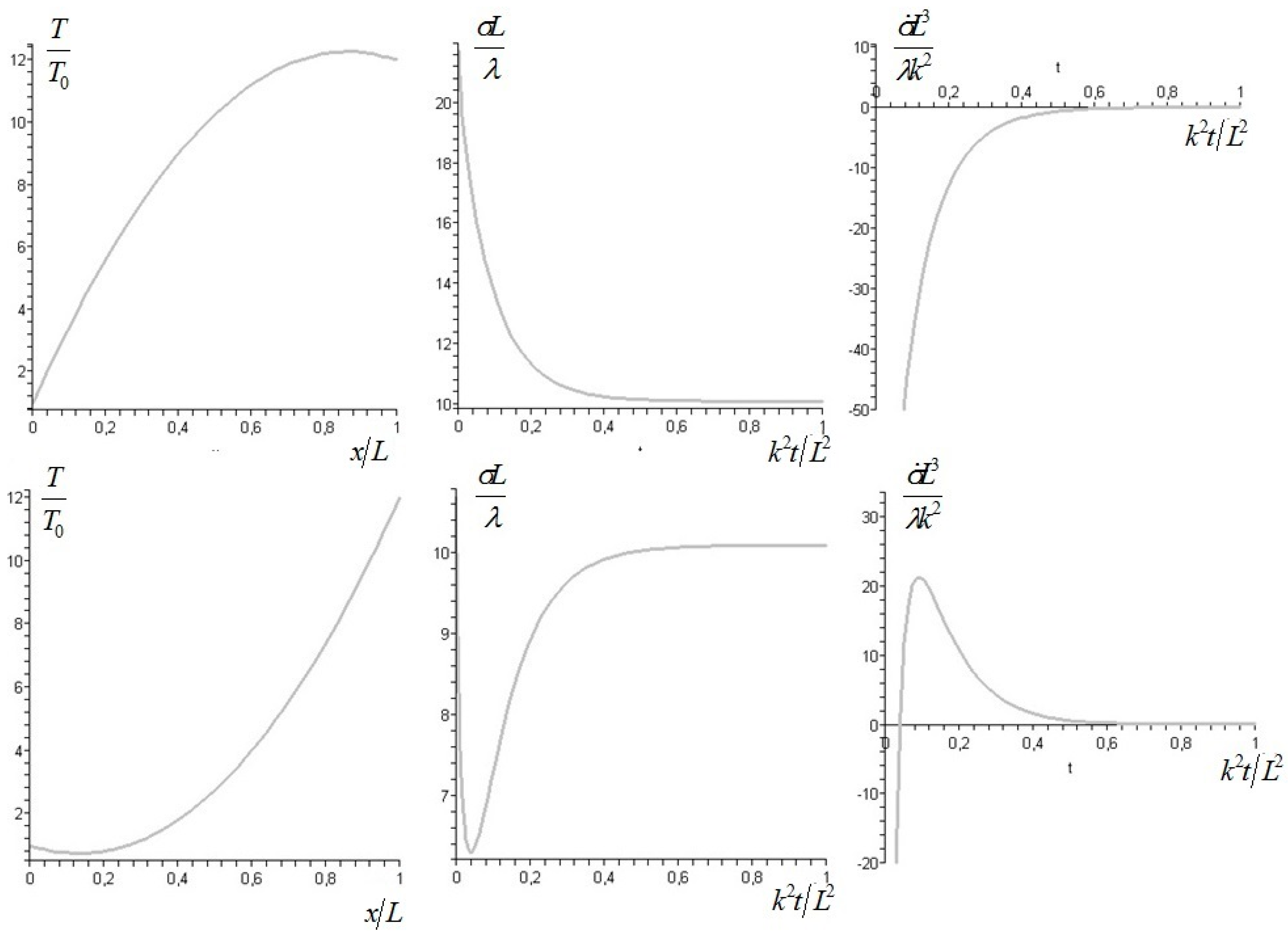
and the plots of the initial profile of temperature, of the entropy production and its derivative for two different cases corresponding to and are reported in Figure 1. The values are scaled to the a-dimensional quantities for the entropy production, to for its derivative and to for the temperature. The parameters are set as and . The plots are obtained truncating the series at . As can be seen, in the case is positive the value of approaches, as becomes large, the value zero from below, whether in the case is negative the value of approaches the zero from above.
Another example is given by the distribution composed by just one Fourier component, that is
where . From Equation (41) it follows directly that the sign of S is opposite to the sign of .
Now we will show also that it is possible to get, with a proper choice of the constants , and in Formula (44), an initial value of ; that is, , positive. We take a small value of and make the series in in the expression for . At first order we get, for ,
where again we set . Integrating by parts the second addend of the right hand side we have
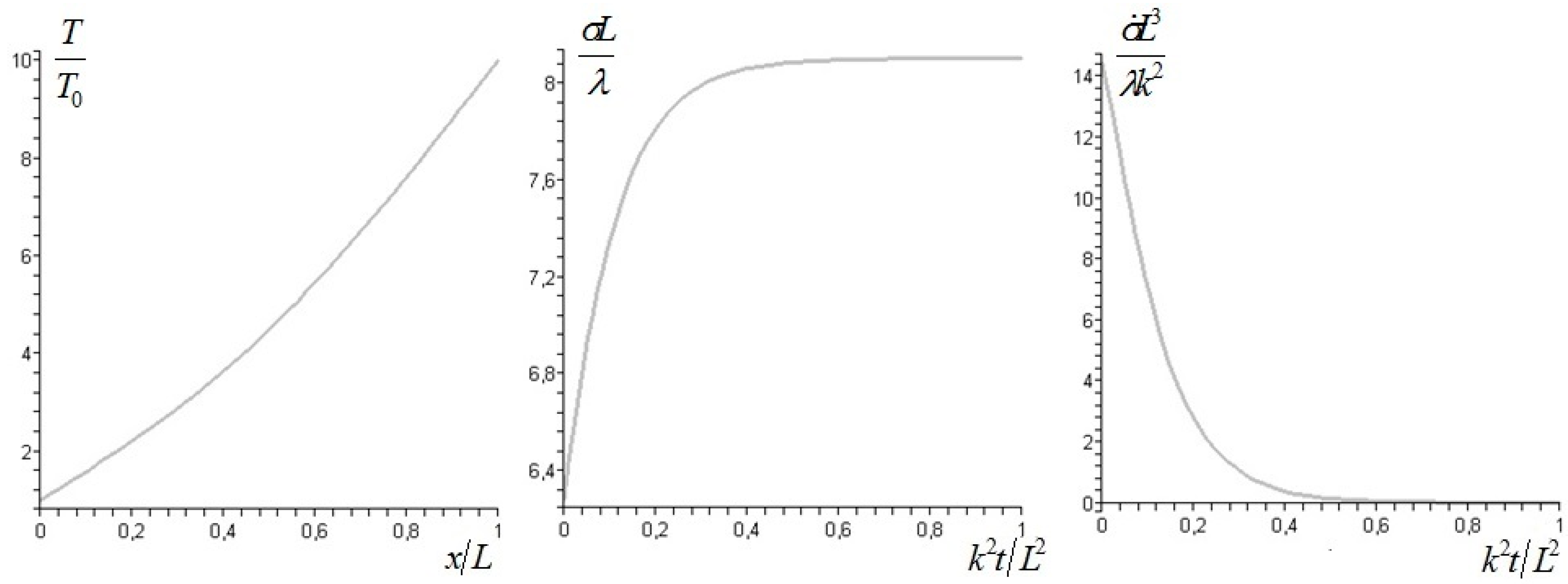
where the positive function f(a) has been defined just after Equation (40). So, for small values of q, the sign of is opposite to the sign of q: it may be either positive or negative. From these two example, we see that it could happen that both the values of for and may be positive. Thus, in principle, it may happen that the function stay positive for all values of ; that is, the entropy production is an increasing function of in these cases. Indeed, an example is reported in Figure 2, where the parameters are set as and .
Let us summarize the findings of this section: the behavior in time at infinity of the entropy production is dominated by the exponential function corresponding to the first eigenvalue, i.e., : by looking at the sign of the quantity , defined in Equations (35) and (36), it is possible to determine if approaches the zero from below or above; that is, if approaches its constant value as a decreasing or an increasing function of time for large times. The entropy production has a minimum value for some finite time if is positive and the initial value of is negative (Figure 1), in the second both the signs are negative (positive) the entropy production may be a decreasing (increasing) function of time. In the case is zero (e.g., when the environmental temperature has a constant value), the entropy production is dominated by the exponential and one has to look at the sign of the limit instead of .
5. Conclusions
We analyzed the evolution of the temperature inside a homogeneous solid according to the linear Fourier equation. The quantity of interest in the paper is the entropy production given by Equation (17). We showed how this quantity does not follow in general an extremum principle. It is important to underline that in this paper we do not issue the general validity of the Prigogine’s minimum entropy production principle: if on a system act forces and flows, if the relations among forces and flows are linear, if the phenomenological coefficients are constant and if the Onsager reciprocal relations are valid then undoubtedly the entropy production of the system reaches a minimum at the non-equilibrium steady state (see, e.g., [2] or [6]). In the case of the heat diffusing in a solid according to the linear Fourier law, what is missing is postulate (b); that is, the fact that the phenomenological coefficient is not a constant but depends on the temperature itself: A constant phenomenological coefficient and the linear Fourier law expressed by Equation (9) are two mutually exclusive possibilities. In this work, we assumed the validity of the linear Fourier law showing in this case that the entropy production, given by (17), cannot be characterized by an extremum principle: instead, the evolution of this quantity can be characterized by looking at the coefficients of the generalized Fourier modes and may be also an increasing function of time. In the language of system theory, we could say that the entropy production, given by Equation (17), is not a Lyapunov function for the linear heat Equation (9). An example of a Lyapunov function for Equation (9) is given by Equation (14) but others could be given. As a last remark, we would like to underline that the entropy production is closely related to the exergy destruction of the system [14]; that is, with the “destruction” of the maximum theoretical useful work that can be obtained by the solid in the process of bringing it to the thermodynamic equilibrium with the environment. In this view, the possibility to identify states characterized by an interesting exergy content seems to be new and will be the scope of next works.
Conflicts of Interest
The author declares no conflict of interest.
References
- Prigogine, I. Etude Thermodynamique des Phenomenes Irreversibles. Dunod: Paris, France, 1947. [Google Scholar]
- Martyushev, L.M.; Nazarova, A.S.; Seleznev, V.D. On the problem of the minimum entropy production in the nonequilibrium stationary state. J. Phys. A Math. Theor. 2007, 40, 371–380. [Google Scholar] [CrossRef]
- Bertola, V.; Cafaro, E. A critical analysis of the minimum entropy production theorem and its application to heat and fluid flow. Int. J. Heat Mass Transf. 2008, 51, 1907–1912. [Google Scholar] [CrossRef]
- Martyushev, L.M. Entropy and Entropy Production: Old Misconceptions and New Breakthroughs. Entropy 2013, 15, 1152–1170. [Google Scholar] [CrossRef]
- Glansdorff, P.; Prigogine, I. Sur Les Propriétés Différentielles De La Production d'Entropie. Physica 1954, 20, 773–780. [Google Scholar] [CrossRef]
- Kondepudi, D.; Prigogine, I. Modern Thermodynamics: From Heat Engines to Dissipative Structures; John Wiley and Sons: New York, NY, USA, 1999. [Google Scholar]
- Prigogine, I. Introduction to Thermodynamics of Irreversible Processes; Interscience: New York, NY, USA, 1955. [Google Scholar]
- Glansdorff, P.; Prigogine, I. Thermodynamics of Structure, Stability and Fluctuations; John Wiley and Sons: Hoboken, NJ, USA, 1971. [Google Scholar]
- De Groot, S.R.; Mazur, P. Non-Equilibrium Thermodynamics; Dover: New York, NY, USA, 2013. [Google Scholar]
- Robinson, J.C. Infinite-Dimensional Dynamical Systems: An Introduction to Dissipative Parabolic PDEs and the Theory of Global Attractors; Cambridge University Press: Cambridge, UK, 2001. [Google Scholar]
- Fiedler, B. Handbook of Dynamical Systems; Elsevier: Amsterdam, The Netherlands, 2002. [Google Scholar]
- Xu, M. The thermodynamic basis of entransy and entransy dissipation. Energy 2011, 36, 4272–4277. [Google Scholar] [CrossRef]
- Bergman, T.L.; Incropera, F.P.; DeWitt, D.P.; Lavine, A.S. Fundamentals of Heat and Mass Transfer; John Wiley and Sons: Hoboken, NJ, USA, 2011. [Google Scholar]
- Sciubba, E.; Wall, G. A brief commented history of exergy: From the beginning to 2004. Int. J. Thermodyn. 2007, 10, 1–26. [Google Scholar]
Figure 1.
From left to right: plots of the initial profile of temperature, of the entropy production and its derivative corresponding to the temperature described by Equation (44). In the first three plots above, the parameters are set as and ; for the plots below, and .
Figure 1.
From left to right: plots of the initial profile of temperature, of the entropy production and its derivative corresponding to the temperature described by Equation (44). In the first three plots above, the parameters are set as and ; for the plots below, and .

Figure 2.
From left to right: plots of the initial profile of temperature, of the entropy production and its derivative corresponding to the temperature described by Equation (45). The parameters are set as and .
Figure 2.
From left to right: plots of the initial profile of temperature, of the entropy production and its derivative corresponding to the temperature described by Equation (45). The parameters are set as and .

© 2016 by the author; licensee MDPI, Basel, Switzerland. This article is an open access article distributed under the terms and conditions of the Creative Commons by Attribution (CC-BY) license (http://creativecommons.org/licenses/by/4.0/).
Share and Cite
MDPI and ACS Style
Zullo, F. Entropy Production in the Theory of Heat Conduction in Solids. Entropy 2016, 18, 87. https://0-doi-org.brum.beds.ac.uk/10.3390/e18030087
AMA Style
Zullo F. Entropy Production in the Theory of Heat Conduction in Solids. Entropy. 2016; 18(3):87. https://0-doi-org.brum.beds.ac.uk/10.3390/e18030087
Chicago/Turabian StyleZullo, Federico. 2016. "Entropy Production in the Theory of Heat Conduction in Solids" Entropy 18, no. 3: 87. https://0-doi-org.brum.beds.ac.uk/10.3390/e18030087
Note that from the first issue of 2016, this journal uses article numbers instead of page numbers. See further details here.