1. Introduction
Life exists away from equilibrium. Left isolated, systems will tend toward thermodynamic equilibrium. Open systems can be maintained away from equilibrium via the exchange of energy and matter with the environment. In addition, biological systems typically consist of a large number of interacting parts. This paper presents a way of describing these “parts” as morphisms in a category. A category consists of a collection of objects along with morphisms or arrows between objects, obeying certain conditions. We consider time-homogeneous Markov processes as a general framework for modeling various biological and biochemical systems whose dynamical equations are linear. Viewed as morphisms in a category, the “open Markov processes” discussed in this paper provide a framework for describing open systems which can be combined to build larger systems.
Intuitively, one can think of a Markov process as specifying the dynamics of a probability or “population” distribution that is spread across a finite set of states. A population distribution is a non-normalized probability distribution, see for example [
1]. The population of a particular state can be any non-negative real number. The total population in an open Markov process is not constant in time as population can flow in and out through certain boundary states. Part of the utility of Markov processes as models of physical or biological systems stems from the flexibility in choosing the correspondence between the states of the Markov process and the actual system it is to model. For instance, the states of a Markov process could correspond to different internal states of a particular molecule or chemical species. In this case, the transition rates describe the rates at which the molecule transitions among these states. Or, the states of a Markov process could correspond to a molecule’s physical location. In this case, the transition rates encode the rates at which that molecule moves from place to place.
This paper is structured as follows. In
Section 2, we give some preliminary definitions from the theory of Markov processes and explain the concept of an open Markov process. In
Section 3, we introduce a model of membrane transport as a simple example of an open Markov process. In
Section 4, we introduce the category
. The objects in
are finite sets of “states” whose elements are labeled by non-negative real numbers which we call “populations”. The morphisms in
are Markov processes equipped with a detailed balanced equilibrium distribution as well as maps specifying input and output states. If the outputs of one process match the inputs of another process the two can be composed, yielding a new open Markov process. We refer to the union of the input and output states as the “boundary” of an open Markov process.
In
Section 5, we show that if the populations at the boundary of an open detailed balanced Markov process are held fixed, then the non-equilibrium steady states which emerge minimize a quadratic form, which we call the “dissipation”, subject to the constraint on the boundary populations. Depending on the values of the boundary populations, these non-equilibrium steady states can exist arbitrarily far from the detailed balanced equilibrium of the underlying Markov process. In
Section 6, we show that, for fixed boundary populations, this principle of minimum dissipation approximates Prigogine’s principle of minimum entropy production in the neighborhood of equilibrium plus a correction term involving only the flow of relative entropy through the boundary of the open Markov process.
2. Open Markov Processes
In this section, we define open Markov processes, describe the detailed balanced condition for equilibria and define non-equilibrium steady states for Markov processes.
An
open Markov process, or open, continuous time, discrete state Markov chain, is a triple
where
V is a finite set of
states,
is the subset of
boundary states and
is an
infinitesimal stochastic HamiltonianFor each
, the dynamical variable
is the
population at the
state. We call the resulting function
the
population distribution. Populations evolve in time according to the
open master equationThe off-diagonal entries
are the rates at which population transitions from the
to the
state. A
steady state distribution is a population distribution which is constant in time:
A
closed Markov process, or continuous time, discrete state Markov chain, is an open Markov process whose boundary is empty. For a closed Markov process, the open master equation becomes the usual master equation
In a closed Markov process, the total population is conserved:
enabling one to talk about the relative probabilities of being in particular states. A steady-state distribution in a closed Markov process is typically called an
equilibrium. We say an equilibrium
of a Markov process is
detailed balanced if
An
open detailed balanced Markov process is an open Markov process
together with a detailed balanced equilibrium
on
V. In
Section 5, we define the “dissipation”, which depends on the detailed balanced equilibrium populations, hence we equip an open Markov process with a specific detailed balanced equilibrium of the underlying closed Markov process. Thus, if a Markov process admits multiple detailed balanced equilibria, we choose a specific one. Note that we consider only detailed balanced equilibria such that the populations of all states are non-zero. Later, it will become clear why this is important.
For a pair of distinct states
, the term
is the flow of population from
j to
i. The
net flow of population from the
state to the
is
Summing the net flows into a particular state we can define the
net inflow of a particular state to be
Since
the right side of this equation is the time derivative of the population at the
state. Writing the master equation in terms of
or
we have
The net flow between each pair of states vanishes identically in a detailed balanced equilibrium
q:
For a closed Markov process, the existence of a detailed balanced equilibrium is equivalent to a condition on the rates of a Markov process known as
Kolmogorov’s criterion [
2], namely that
for any finite sequence of states
of any length. This condition says that the product of the rates along any cycle is equal to the product of the rates along the same cycle in the reverse direction.
A non-equilibrium steady state is a steady state in which the net flow between at least one pair of states is non-zero. Thus, there could be population flowing between pairs of states, but in such a way that these flows still yield constant populations at all states. In a closed Markov process, the existence of non-equilibrium steady states requires that the rates of the Markov process violate Kolmogorov’s criterion. We show that open Markov processes with constant boundary populations admit non-equilibrium steady states even when the rates of the process satisfy Kolmogorov’s criterion. Throughout this paper, we use the term equilibrium to mean detailed balanced equilibrium.
3. Membrane Diffusion as an Open Markov Process
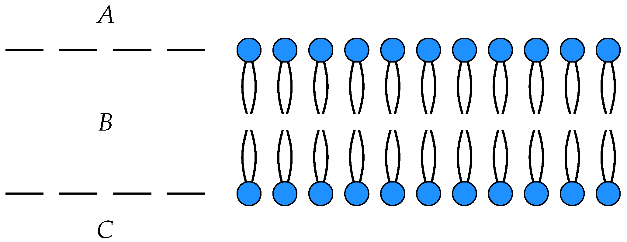
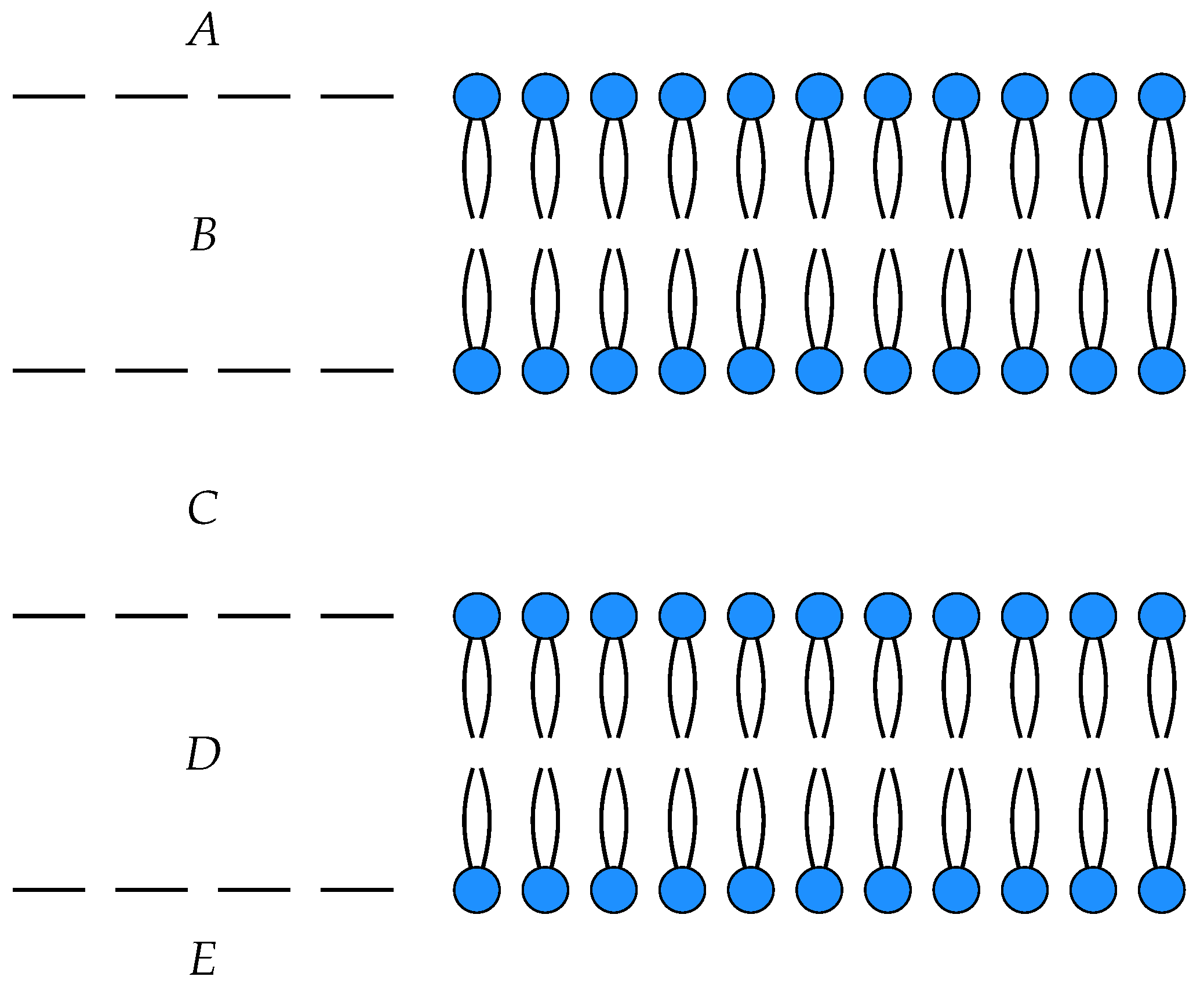
To illustrate these ideas, we consider a simple model of the diffusion of neutral particles across a membrane as an open detailed balanced Markov process
with three states
, input
A and output
C. The states
A and
C correspond to the each side of the membrane, while
B corresponds within the membrane itself, see
Figure 1.
In this model,
is the number of particles on one side of the membrane,
the number of particles within the membrane and
the number of particles on the other side of the membrane. The off-diagonal entries in the Hamiltonian
are the rates at which population hops from
j to
i. For example,
is the rate at which population moves from
B to
A, or from inside the membrane to the top of the membrane. Let us assume that the membrane is symmetric in the sense that the rate at which particles hop from outside of the membrane to the interior is the same on either side,
i.e.,
and
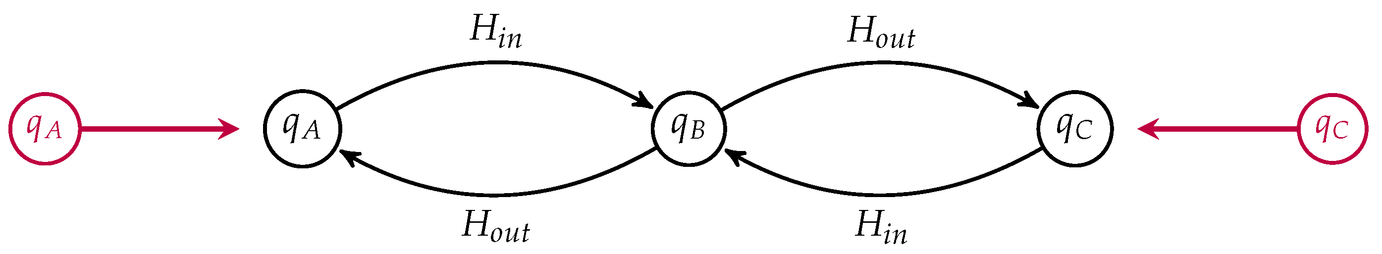
. We can draw such an open Markov process as a labeled graph, see for instance
Figure 2.
The labels on the edges are the corresponding transition rates. The states are labeled by their detailed balanced equilibrium populations, which, up to an overall scaling, are given by
and
. Suppose the populations
and
are externally maintained at constant values,
i.e., whenever a particle diffuses from outside the cell into the membrane, the environment around the cell provides another particle and similarly when particles move from inside the membrane to the outside. We call
the
boundary populations. Given the values of
and
, the steady state population
compatible with these values is
In
Section 5, we show that this steady state population minimizes the dissipation, subject to the constraints on
and
.
We thus have a non-equilibrium steady state
with
given in terms of the boundary populations above. From these values, we can compute the boundary flows,
as
and
Written in terms of the boundary populations this gives
and
Note that
implying that there is a constant net flow through the open Markov process. As one would expect, if
there is a positive flow from
A to
C and
vice versa. Of course, in actual membranes there exist much more complex transport mechanisms than the simple diffusion model presented here. A number of authors have modeled more complicated transport phenomena using the framework of networked master equation systems [
3,
4].
In our framework, we call the collection of all boundary population-flows pairs the steady state “behavior” of the open Markov process. In recent work [
5], Baez, Fong and the author construct a functor
from the category of open detailed balanced Markov process to the category of linear relations. Applied to an open detailed balanced Markov process, this functor yields the set of allowed steady state boundary population-flow pairs. One can imagine a situation in which only the populations and flows of boundary states are observable, thus characterizing a process in terms of its behavior. This provides an effective “black-boxing” of open detailed balanced Markov processes.
As morphisms in a category, open detailed balanced Markov processes can be composed, thereby building up more complex processes from these open building blocks. The fact that “black-boxing” is accomplished via a functor means that the behavior of a composite Markov process can be built up from the composite behaviors of the open Markov processes from which it is built. In this paper, we illustrate how this framework can be utilized to study linear master equation systems far from equilibrium with a particular emphasis on the modeling of biological phenomena.
Markovian or master equation systems have a long history of being used to model and understand biological systems. We make no attempt to provide a complete review of this line of work. Schnakenberg, in his paper on networked master equation systems, defines the entropy production in a Markov process and shows that a quantity related to entropy serves as a Lyapunov function for master equation systems [
6]. His book [
4] provides a number of biochemical applications of networked master equation systems. Oster, Perelson and Katchalsky developed a theory of “networked thermodynamics” [
7], which they went on to apply to the study of biological systems [
3]. Perelson and Oster went on to extend this work into the realm of chemical reactions [
8].
Starting in the 1970s, T. L. Hill spearheaded a line of research focused on what he called “free energy transduction” in biology. A shortened and updated form of his 1977 text on the subject [
9] was republished in 2005 [
10]. Hill applied various techniques, such as the use of the cycle basis, in the analysis of biological systems. His model of muscle contraction provides one example [
11].
One quantity central to the study of non-equilibrium systems is the rate of entropy production [
12,
13,
14,
15]. Prigogine’s principle of minimum entropy production [
16] asserts that for non-equilibrium steady states that are near equilibrium, entropy production is minimized. This is an approximate principle that is obtained by linearizing the relevant equations about an equilibrium state. In fact, for open detailed balanced Markov processes, non-equilibrium steady states are governed by a
different minimum principle that holds
exactly, arbitrarily far from equilibrium. We show that for fixed boundary conditions, non-equilibrium steady states minimize a quantity we call “dissipation”. If the populations of the non-equilibrium steady state are close to the population of the underlying detailed balanced equilibrium, one can show that dissipation is close to the rate of change of relative entropy plus a boundary term. Dissipation is in fact related to the Glansdorff–Prigogine criterion, which states that a non-equilibrium steady state is stable if the second order variation of the entropy production is non-negative [
6,
12].
Many of the mathematical results underlying the theory of non-equilibrium steady states can be found in the book by D. Jiang, M. Qian and M.P. Qian [
17]. More recently, results concerning fluctuations have been extended to master equation systems [
18]. In the past two decades, H. Qian of the University of Washington and collaborators have published numerous results on non-equilibrium thermodynamics, biology and related topics [
19,
20,
21].
This paper is part of a larger project which uses category theory to unify a variety of diagrammatic approaches found across the sciences including, but not limited to, electrical circuits, control theory and bond graphs [
22,
23]. We hope that the categorical approach will shed new light on each of these subjects as well as their interrelation, particularly as we generalize the results presented in this and recent papers to the more general, non-linear, setting of open chemical reaction networks.
4. The Category of Open Detailed Balanced Markov Processes
In this section, we describe how open detailed balanced Markov processes are the morphisms in a certain type of symmetric, monoidal, dagger-compact category. In previous work, Baez, Fong and the author [
5] used the framework of decorated cospans [
24] to construct the category
. Here, we give an intuitive description of this category and refer to those papers for the mathematical details.
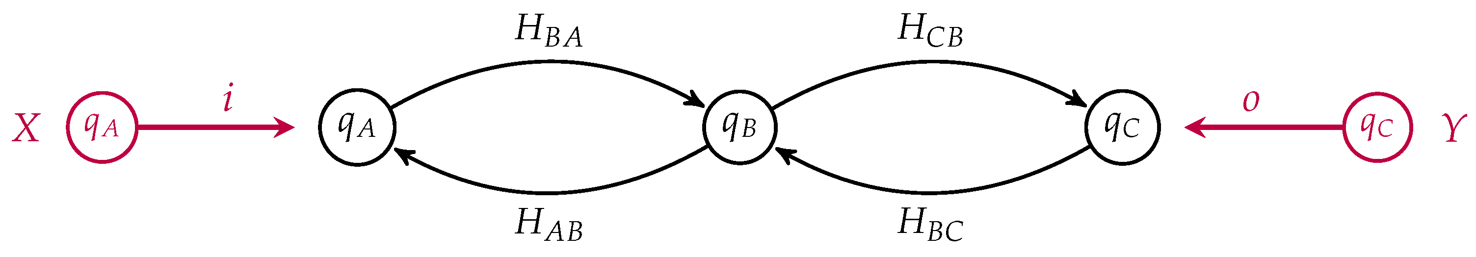
An object in is a finite set with populations, i.e., a finite set X together with a map assigning a population to each element . A morphism consists of an open detailed balanced Markov process together with input and output maps and which preserve population, i.e., and . The union of the images of the input and output maps form the boundary of the open Markov processes .
One can draw an open detailed balanced Markov process as a labeled directed graph whose vertices are labeled by their equilibrium populations and with specified subsets of the vertices as the input and the output states. Recall our simple model of membrane diffusion as an open detailed balanced Markov process, which we draw in
Figure 3, as a morphism from the input
to the output
This is a morphism in
from
X to
Y where
X and
Y are finite sets with populations. In this simple example,
X and
Y both contain a single element, namely
A and
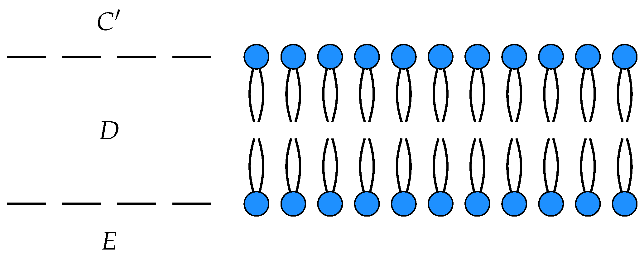
C respectively. Suppose we had another such membrane as depicted in
Figure 4.
This is a morphism in
from with input
and output
. Two open detailed balanced Markov processes can be composed if the detailed balanced equilibrium populations at the outputs of one match the detailed balanced equilibrium populations at the inputs of the other. This requirement guarantees that the composite of two open detailed balanced Markov process still admits a detailed balanced equilibrium, see
Figure 5.
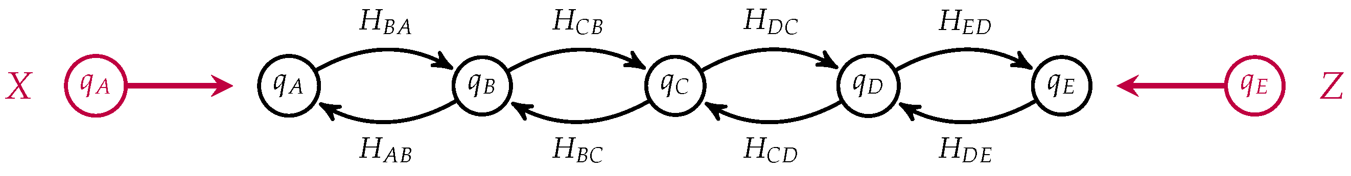
If
in our two membrane models, we can compose them by identifying
C with
to yield an open detailed balanced Markov process modeling the diffusion of neutral particles across membranes arranged in series, see
Figure 6.
Notice that the states corresponding to
C and
in each process have been identified and become internal states in the composite which is a morphism from
to
. This open Markov process can be thought of as modeling the diffusion across two membranes in series, see
Figure 7.
One can “black-box” an open detailed balanced Markov process by converting it into an electrical circuit, applying the already known black-boxing functor for electrical circuits [
23] and translating the result back into the language of open Markov processes [
5]. The key step in this process is the construction of a quadratic form which we call “dissipation”, analogous to power in electrical circuits, which is minimized when the populations of an open Markov process are in a steady state.
5. Principle of Minimum Dissipation
Here, we show that by externally fixing the populations at boundary states, one induces steady states which minimize a quadratic form which we call “dissipation”.
Definition 1. Given an open detailed balanced Markov process we define the dissipation functional of a population distribution p to be Given boundary populations
, we can minimize this functional over all
p which agree on the boundary. Differentiating the dissipation functional with respect to an internal population, we get
Multiplying by
yields
where we recognize the right-hand side from the open master equation for internal states. We see from Equation (
1) that, for fixed boundary populations, the conditions for
p to be a steady state, namely that
is equivalent to the condition that
Definition 2. We say a population distribution obeys the principle of minimum dissipation with boundary population if p minimizes subject to the constraint that .
With this, we can state the following theorem:
Theorem 3. A population distribution is a steady state with boundary population if and only if p obeys the principle of minimum dissipation with boundary population b.
Proof. This follows from Theorem 28 in [
5]. ☐
Given specified boundary populations, one can compute the steady state boundary flows by minimizing the dissipation subject to the boundary conditions.
Definition 4. We call a population-flow pair a steady state population-flow pair if the flows arise from a population distribution which obeys the principle of minimum dissipation.
Definition 5. The behavior of an open detailed balanced Markov process with boundary B is the set of all steady state population-flow pairs along the boundary.
Indeed, there is a functor
which maps open detailed balanced Markov processes to their steady state behaviors. This is the main result of our previous paper [
5]. The fact that this is a functor means that the behavior of a composite open detailed balanced Markov process can be computed as the composite of the behaviors.
6. Dissipation and Entropy Production
In the last section, we saw that non-equilibrium steady states with fixed boundary populations minimize the dissipation. In this section, we relate the dissipation to a divergence between population distributions known in various circles as the relative entropy, relative information or the Kullback–Leibler divergence. The relative entropy is not symmetric and violates the triangle inequality, which is why it is called a “divergence” rather than a metric, or distance function. We show that for population distributions near a detailed balanced equilibrium, the rate of change of the relative entropy is approximately equal to the dissipation plus a “boundary term”.
The
relative entropy of two distributions
is given by
It is well known that, for a closed Markov process admitting a detailed balanced equilibrium, the relative entropy with respect to this detailed balanced equilibrium distribution is monotonically decreasing with time, see for instance [
2]. There is an unfortunate sign convention in the definition of relative entropy: while entropy is typically increasing, relative entropy typically decreases. More generally, the relative entropy between any two population distributions is non-increasing in a closed Markov process.
In an open Markov process, the sign of the rate of change of relative entropy is indeterminate. Consider an open Markov process
. For any two population distributions
and
which obey the open master equation let us introduce the quantities
and
which measure the rate at which population flows into the
state from outside the system. These quantities are sometimes referred to as the boundary-fluxes. Notice that
for
, as the populations of internal states evolve according to the master equation. In terms of these quantities, the rate of change of relative entropy for an open Markov process can be written as
The first term is the rate of change of relative entropy for a closed Markov process. This is less than or equal to zero [
25,
26]. Thus, the rate of change of relative entropy in an open Markov process satisfies
This inequality tells us that the rate of change of relative entropy in an open Markov processes is bounded by the rate at which relative entropy flows through its boundary. If
q is an equilibrium solution of the master equation
then the rate of change of relative entropy can be written as
Furthermore, if
q satisfies detailed balance we can write this as
where
is the
thermodynamic flux from
j to
i and
is the conjugate
thermodynamic force. This quantity:
is what Schnakenberg calls “the rate of entropy production” [
6]. This is always non-negative. Note that due to the sign convention in the definition of relative entropy, in the absence of the boundary term, a positive rate of entropy production corresponds to a decreasing relative entropy.
We shall shortly relate the rate of change of relative entropy to the dissipation for open detailed balanced Markov processes, but first let us consider the quantity . It is the entropy production per unit flow from j to i. If , i.e., if there is a positive net flow of population from j to i, then . In addition, implies that . Thus, we see that this form of entropy production is, by definition, non-negative.
We can understand
as the force resulting from a difference in chemical potential. Let us elaborate on this point to clarify the relation of our framework to the language of chemical potentials used in non-equilibrium thermodynamics. Markov processes are special cases of chemical reactions obeying mass action kinetics in which each reaction is unimolecular. Let us assume that we are dealing with only unimolecular reactions and that our system is an ideal mixture so that the chemical potential
associated to the
state or species is given by:
where
T is the temperature of the system in units where Boltzmann’s constant is equal to one,
is some reference chemical potential of the
species and
is the
molar fraction of the
species with
giving the number of moles of the
species [
13]. Note that this is equal to the fraction of the population in the
state
. The difference in chemical potential between two states gives the force associated with the flow which seeks to reduce this difference in chemical potential
This potential difference vanishes when
and
are in equilibrium and we have
or that
If the equilibrium distribution
q satisfies detailed balance, then this also gives an expression for the ratio of the transition rates
in terms of the standard chemical potentials. Thus, we can translate between differences in chemical potential and ratios of populations via the relation
which, if
q satisfies detailed balance gives
We recognize the right hand side as the force
times the temperature of the system
T:
Let us return to our expression for
where
q is an equilibrium distribution:
Consider the situation in which
p is near to the equilibrium distribution
q and let
denote the deviation in the ratio
from unity so that
We collect these deviations in a vector denoted by
ϵ. Expanding the logarithm to first order in
ϵ we have that
which gives
By
, we mean a sum of terms of order
. When
q is a detailed balanced equilibrium, we can rewrite this quantity as
We recognize the first term as the negative of the dissipation
which yields
We see that for open Markov processes, minimizing the dissipation approximately minimizes the rate of decrease of relative entropy plus a term which depends on the boundary populations. In the case that boundary populations are held fixed so that
, we have that
In this case, the rate of change of relative entropy can be written as
Summarizing the results of this section, we have that for
p arbitrarily far from the detailed balanced equilibrium equilibrium
q, the rate of relative entropy reduction can be written as
For
p in the vicinity of a detailed balanced equilibrium, we have that
where
is the dissipation and
measures the deviations of the populations
from their equilibrium values. We have seen that in a non-equilibrium steady state with fixed boundary populations, dissipation is minimized. We showed that for steady states near equilibrium, the rate of change of relative entropy is approximately equal to minus the dissipation plus a boundary term. Minimum dissipation coincides with minimum entropy production only in the limit
.
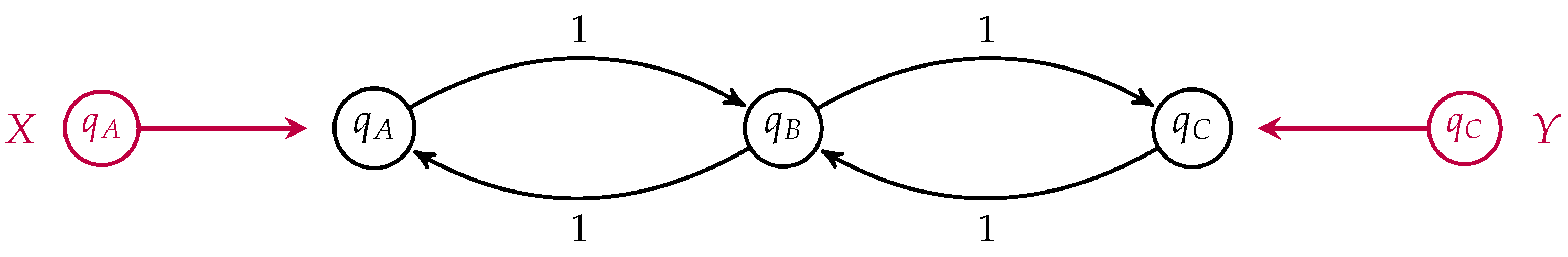
7. Minimum Dissipation versus Minimum Entropy Production
We return to our simple three-state example of membrane transport to illustrate the difference between populations which minimize dissipation and those which minimize entropy production, depicted in
Figure 8.
For simplicity, we have set all transition rates equal to one. In this case, the detailed balance equilibrium distribution is uniform. We take
. If the populations
and
are externally fixed, then the population
which minimizes the dissipation is simply the arithmetic mean of the boundary populations
The rate of change of the relative entropy
where
q is the uniform detailed balanced equilibrium is given by
Differentiating this quantity with respect to
for fixed
and
yields the condition
The solution of this equation gives the population
, which extremizes the rate of change of relative entropy, namely
where
is the Lambert
W-function or the omega function which satisfies the following relation
The Lambert W-function is defined for and double valued for . This simple example illustrates the difference between distributions which minimize dissipation subject to boundary constraints and those which extremize the rate of change of relative entropy. For fixed boundary populations, dissipation is minimized in steady states arbitrarily far from equilibrium. For steady states in the neighborhood of the detailed balanced equilibrium, the rate of change of relative entropy is approximately equal to minus the dissipation plus a boundary term.


