1. Introduction
Quantum thermodynamics can address a single microscopic quantum device performing thermodynamic tasks such as heat transport, power generation, and refrigeration. A dynamical perspective is incorporated in the field of open quantum systems [
1]. The established approach is based on the weak coupling system–bath approximation [
2] leading to Markovian dynamics described by the Lindblad–Goirini–Kossakowski–Sudarshan (L-GKS) master equation [
3,
4]. This approach leads to dynamical evolution which is consistent with the laws of thermodynamics [
1,
5]. In the present paper, we deviate from the established scenario and study a quantum device strongly coupled to the heat baths and undergoing non-Markovian dynamics.
First, we study the phenomena of heat transport. The second law of thermodynamics dictates that heat should always flow from the hot to the cold bath. We use this phenomenon to benchmark our model. Once established, we add to the model an external driving field. Then, the device can operate as a refrigerator, pumping heat from the cold bath to the hot bath.
The phenomenon of transport is associated with a gradient of a driving potential. Even a single molecule subject to temperature gradient will experience a heat current flowing from the higher potential to the lower one. Modelling such a heat flow is the subject of this study. A novel idea is heat rectification, the possibility of asymmetric heat transfer when the baths are switched [
6,
7]. Employing such a concept, one can imagine effectively isolating a subsystem in a far-from-equilibrium state. Close to equilibrium, the rectifying effect must vanish. In a series of papers, Segal and co-workers studied the conditions for heat rectification, tracing the effect to non-linear phenomena either related to asymmetric baths (case A) or to asymmetric system–bath coupling (case B) [
8,
9]. In the present paper, heat transport of case B is analysed based on the non-Markovian stochastic surrogate Hamiltonian approach [
10,
11].
The popular theoretical approach to describe heat transport in a network is to compose the transport equations from local equations. This local approach is correct when only populations are involved. However, when quantum systems are involved, the local approach leads to the violation of the second law of Thermodynamics [
12]. A thermodynamically-consistent treatment within the weak coupling system–bath approximation requires first to diagonalize the total subsystem network, obtaining the global transition frequencies of the total system [
1]. An alternative is a careful perturbation analysis [
13]. Only then can the weak coupling procedure be applied to obtain the consistent transport equations. A major assumption in the derivation is a tensor product form of the system and baths at all times. The weak coupling procedure employed in References [
8,
9] is global and consistent with thermodynamics.
The standard treatment of transport is based on the Landauer–Buttiker scattering theory [
14]. Each scattering event that transports energy from one bath to the other is assumed to be independent, resulting in a Poissonian process. This ballistic description ignores intricate dynamics between the molecular device and its leads.
Can one derive a consistent transport theory beyond the weak system bath coupling limit? An attempt in this direction has been described by Segal [
15,
16], who studied a two-level-system coupled to a spin bath in the intermediate coupling limit. The derivation is based on the Non Interacting Blip Approximation (NIBA) approach which allows the explicit evaluation of the memory kernel. The study finds that the rectifying effect exists in the intermediate coupling range and vanishes in the weak coupling limit of the two-level-system to the spin baths. The NIBA method can only be employed for very simple system Hamiltonians, such as a two-level-system or harmonic oscillators. This approach, using the polaron transformation, was employed to construct a model of solar energy harvesting [
17] and a single electron transistor [
18]. Therefore, a more general approach appropriate for an arbitrary system is required. Recently, the Nonequilibrium Green’s Function Approach (NGFA) has been suggested as a framework of quantum thermodynamics [
19]. In this approach, the energy of the system and its coupling to the reservoirs are controlled by a slow external time-dependent force treated to first-order beyond the quasistatic limit.
In the present study of heat transport, a correlated system–bath scenario is employed. We defy the assumption used in all previous studies of an uncorrelated system and baths represented as a tensor product
[
20]. In addition, the system Hamiltonian is represented on a grid, practically achieving a Hilbert space of size
. The transport dynamics is simulated based on the stochastic surrogate Hamiltonian approach [
10,
11]. The method represents the state by a global system–bath wave function. This leads to a strongly entangled state at all times. As a result, the dynamics is non-Markovian. A stochastic layer is employed to trim the calculation and define the bath temperature. We check the validity of the approach by evaluating that the total entropy generation is positive. Once the method is established, the asymmetric rectifying effect with identical spin baths is studied.
By adding an external driving field, the device is transformed to a refrigerator, driving heat from the cold to the hot bath. This device falls in the category of continuous quantum engines [
21]. Optimal performance will be achieved when the driving frequency is in resonance with the frequency difference of the left and right bath. The refrigeration is studied in the strong coupling regime. It is expected that the cooling current deviates from a linear relation with the coupling. Such an effect has been observed using the NIBA approach [
22].
2. Basic Construction
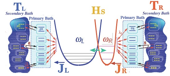
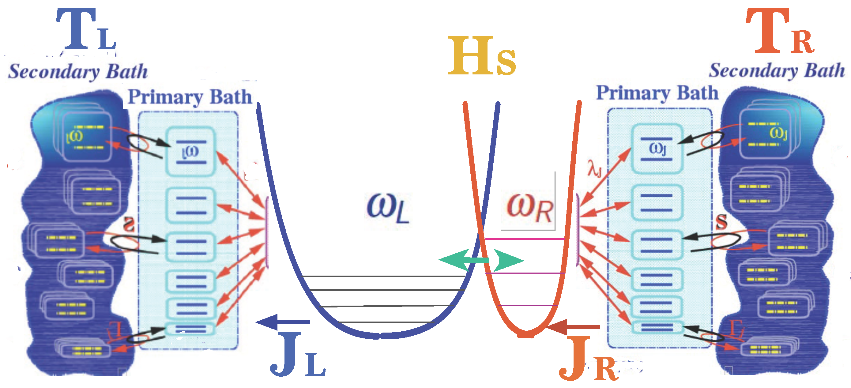
In the stochastic surrogate Hamiltonian approach, the molecular device is subject to dissipative forces due to coupling to two primary baths. In turn, the primary baths are subject to interactions with a secondary bath:
where
represents the system,
and
represent the primary baths,
and
the secondary baths, and
and
the system–bath interaction.
and
are the primary/secondary baths’ interactions. The system Hamiltonian
describes molecular nuclear modes: The molecular Hamiltonian has the form:
Specifically, the molecular device under study is composed of the lower electronic surface of two coupled diabatic oscillators:
where
where parameters are described in
Table 1.
The non-adiabatic coupling potential:
where
,
, and
is the crossing point.
The bath is described by a fully quantum formulation. Briefly, the bath is divided into a primary part interacting with the system directly and a secondary bath which eliminates recurrence and imposes thermal boundary conditions.
The primary bath Hamiltonian is composed of a collection of two-level-systems.
The energies
represent the spectrum of the bath.
and
.
The system bath coupling Hamiltonian has the form:
,
. The system bath coupling function is chosen to be localised exponentially on the right or left potential well
where
,
.
The global state of the system and the hot and cold primary baths are realized by a combined wavefucntion. The dimension of this wavefucntion is of the order of .
The left and right secondary baths are constructed from virtual spins, which are identical to the spin manifold of the right and left baths. The state of this bath is a tensor product of spin wavefunctions with thermal amplitude and random phase [
10]:
where
Z is the partition function
,
is the frequency of the
jth spin, and
are random phases. The temperature
T corresponds to either
or
. Random swap operations are employed to switch between the wavefuctions of the primary and secondary baths [
23]. As a result, the secondary bath defines the temperature of the left or right contacts with the system. Only spins on resonance are swapped; therefore, the transfer of energy can be defined as heat [
24].
The energy balance relation is equivalent to the first law of thermodynamics. The time derivative of the system energy defines two heat currents:
Comment: if the system–bath coupling was a
δ function, Equation (
10) would become the flux operator. In the following, the analysis will be carried out using only the currents
. This means that we avoid the ambiguity of accounting for the system energy. It could be either
or include the interactions
[
25,
26,
27,
28]. The currents in Equation (
10) are invariant to this definition.
Figure 1 shows a schematic view of the systems and primary and secondary baths.
The initial state is the vibrational ground state of the potential
obtained by propagation in imaginary time [
29]. The system wavefunction is represented on a Fourier grid of
points [
30]. The combined computation effort of evaluating the Hamiltonian scales as
where
N is the total size of the Hilbert space which includes system grid points and the dimension of the two baths [
31]. Propagation is carried out by the Chebychev expansion of the evolution operator [
32]. The computational effort scales semi-linearly with
N for each stochastic realization. The number of realizations to achieve convergence is small and scales as
[
10]. In the present study, ten realizations were sufficient.
Table 1 summarizes the computation details.
3. Thermodynamical Aspects of the Surrogate Hamiltonian
The stochastic surrogate Hamiltonian approach relies on a large wavefunction to describe the state of the system and hot and cold primary baths. The typical Hilbert space size is
. The thermalization properties of the Stochastic Surrogate Hamiltonian (SSH) have been studied [
10]. With this size of Hilbert space on the order of 10 realizations are sufficient to converge the local expectation values of system energy and heat currents. The fast convergences can be related to quantum typicality, meaning that the vast majority of all pure states featuring a common expectation value of some generic observable at a given time will yield very similar expectation values of the same observable at any later time [
33,
34,
35].
The temperature of the hot and cold baths is imposed by the secondary baths. The spin of the primary bath is stochastically swapped with an identical spin of the secondary bath. The result is pure heat transfer between the baths, leading to equilibration. In addition, the swap operation generates dephasing of the system [
36].
Transport Dynamics
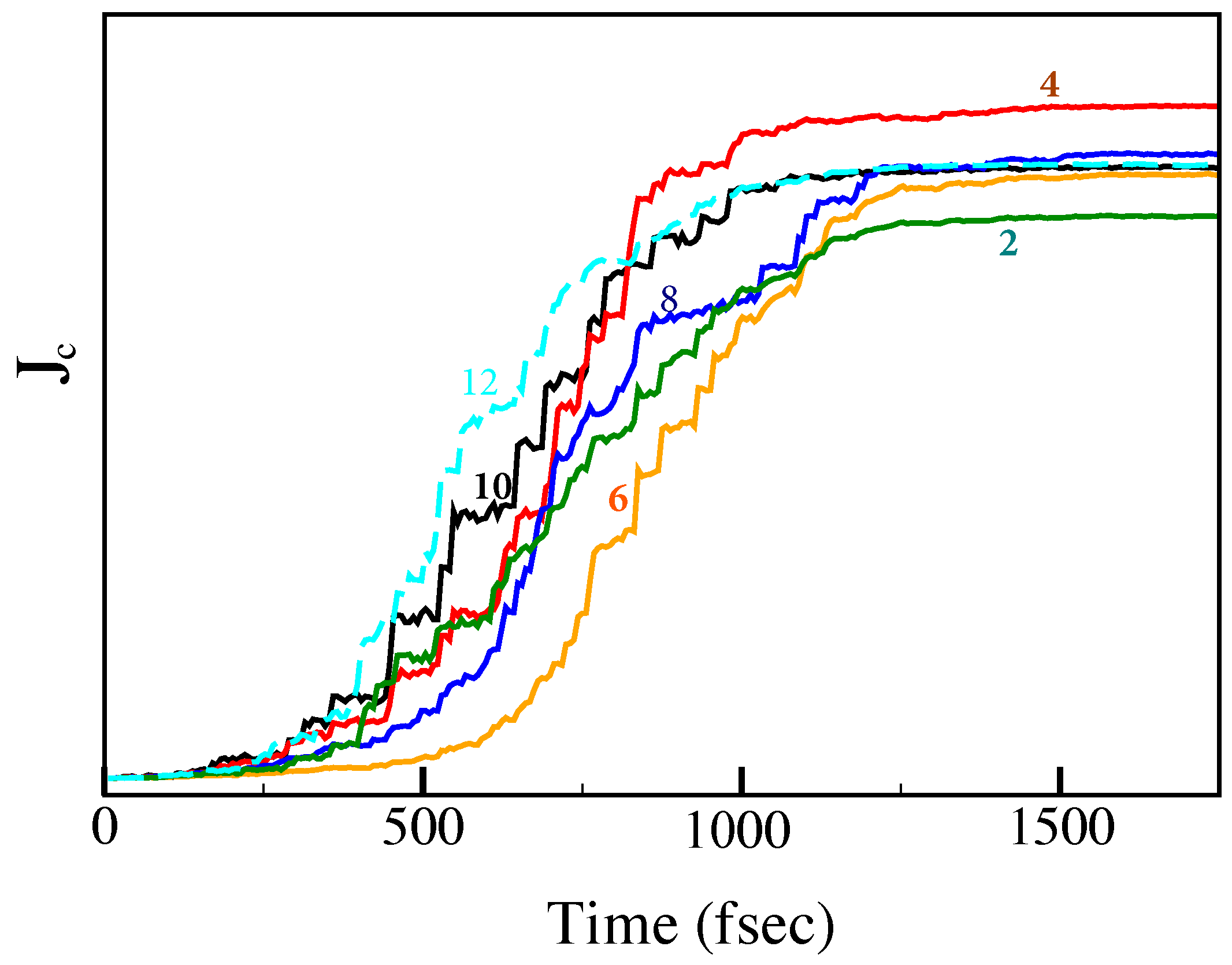
To test the thermodynamical validity of the construction, we study heat transport. Irrespective of the details of the system, heat should flow from the hot to the cold reservoir. At first the molecular model is coupled to the right and left thermal leads. A typical simulation is initiated from an arbitrary wavefunction of the system–bath product state. The dynamics is then switched on for a sufficient propagation period until the combined system reaches a steady state. Each individual realization shows significant fluctuations. Averaging even 10 realizations is sufficient to obtain a smooth average
cf. Figure 2. Heat currents are calculated in steady state, then
. The convergence with respect to the number of realizations is shown in
Figure 2. The steady state current converges within 10 realizations. The transient current requires a much larger number of realizations to converge.
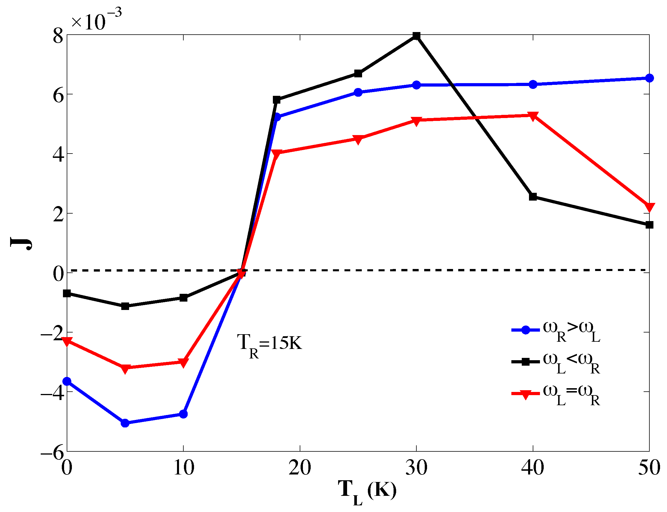
Figure 3 shows the flux
as a function of
for fixed
,
, and
. When
becomes larger than
, the current switches direction in compliance with the II-law of thermodynamics.
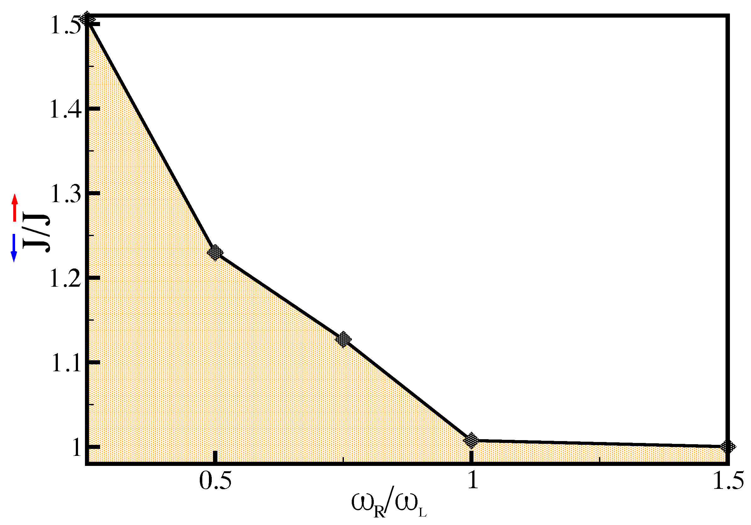
For fixed right and left temperatures, the steady state heat flux is influenced by the frequency ratio . The heat flux is larger when , compared to . This is an indication of the asymmetry of the model and the rectifying effect.
The ratio between the hot to cold current
when the left and right baths are exchanged leaving all other parameters fixed is shown in
Figure 4 as a function of the frequency ratio
. The product
is almost constant.
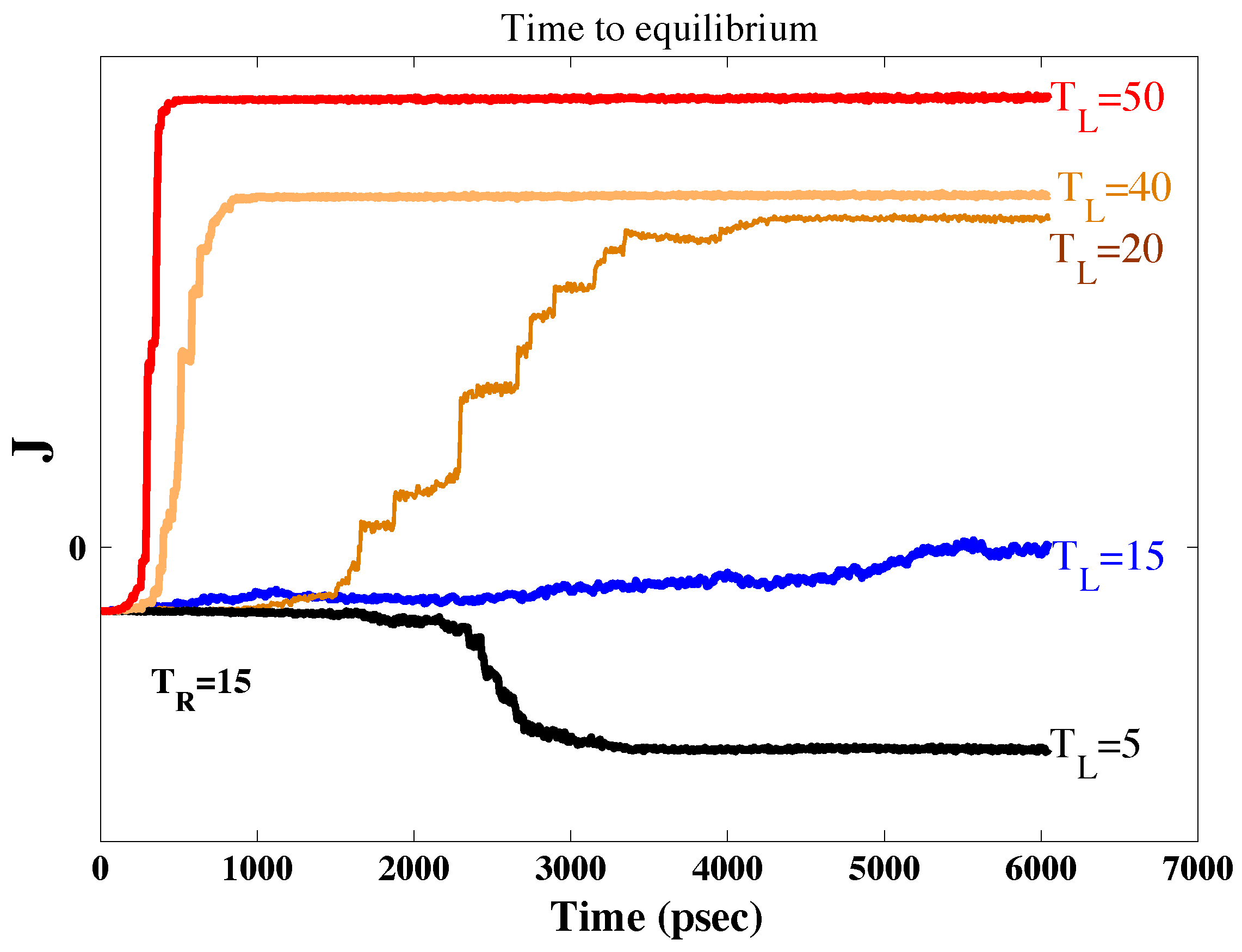
An important dynamical effect is the rate of approach to steady state.
Figure 5 shows the dynamics of approach to steady state where the the right bath temperature
is kept fixed and the left bath temperature is varied. The relaxation rate is faster for larger temperature differences, which would be expected from Newtons heat law.
To conclude, the single molecular heat transport model complies with the first and second law of thermodynamics under all conditions studied.
4. Heat Pump Operation
A heat pump is a device that consumes power to drive heat from a cold to a hot bath. We realize such a device by a single molecule connected to hot and cold leads. The power is applied by a periodic electric field coupled to the molecule through the dipole operator. The heat current through the system is calculated by accounting for the energy flux on each interface in addition to the energy flow from the external time dependent drive:
where
and
. We choose the driving frequency to be in resonance
.
ϵ is the driving amplitude and
μ the dipole constant.
For the heat pump, the energy currents become:
In steady state the entropy production is generated only on the hot and cold baths:
The energy balance becomes .
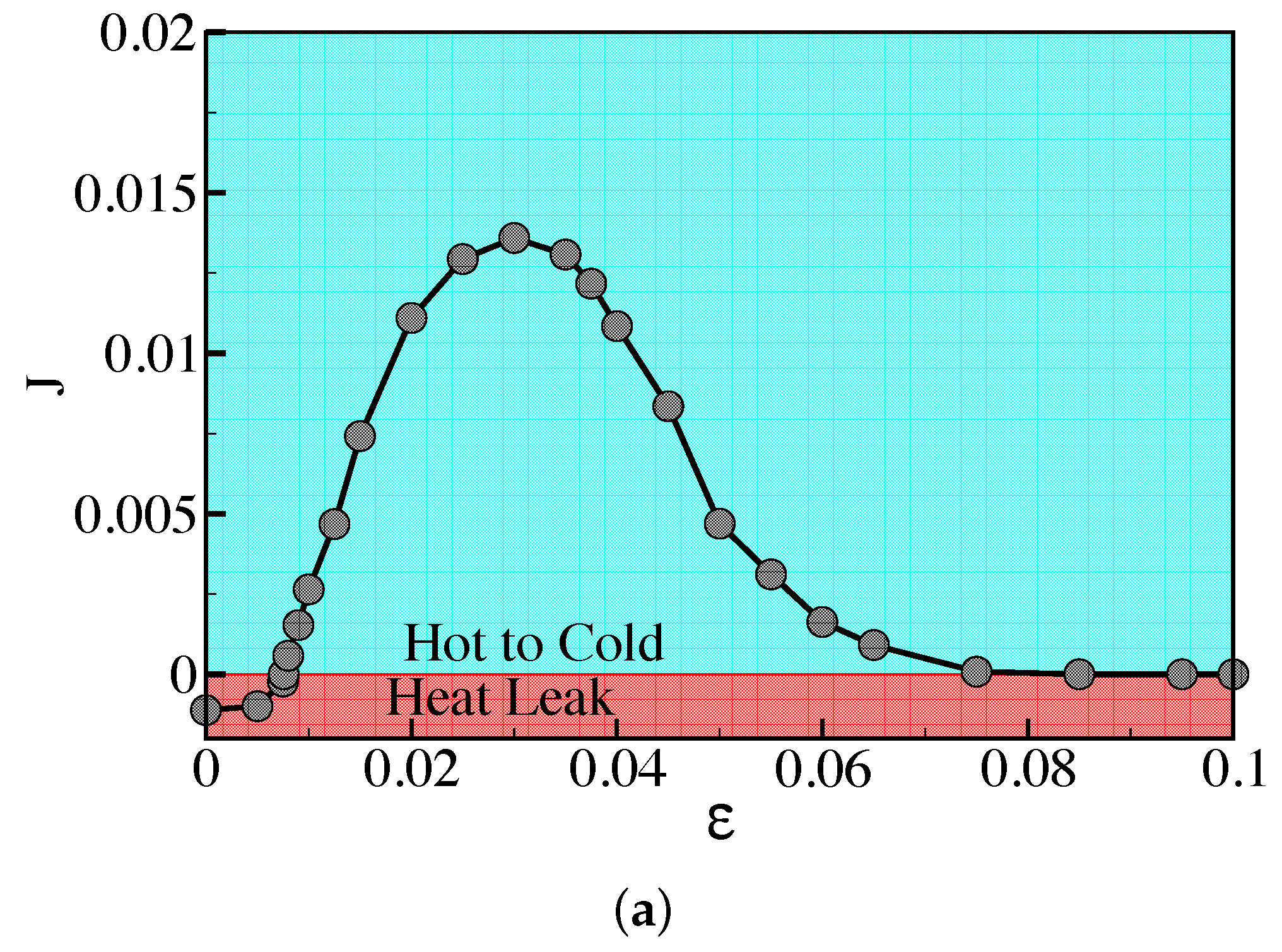
Figure 6 shows the cooling current
as a function of the amplitude
ϵ of the driving field. At weak driving, the heat that leaks from the hot to the cold bath dominates. The driving is not strong enough to overcome the natural heat flow. When the amplitude
ϵ increases, the heat flux
reverses sign, pumping heat from the cold to hot baths. At even stronger driving, the derivative
changes sign. The cooling current is reduced to zero. The strong driving increases the system’s energy and localizes the system on the hot bath.
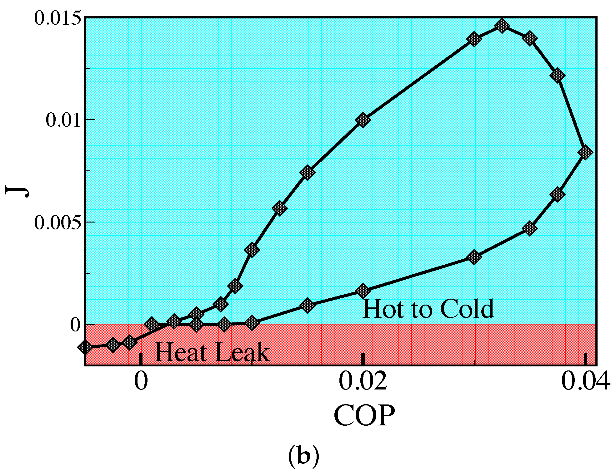
Figure 6b shows the cooling current as a function of the COP, the coefficient of performance, defined as
. The loop in the graph shows two turning points of maximum cooling current and maximum efficiency. This loop is typical of macroscopic classical refrigerators [
37] and was also observed in a model of a four-level quantum refrigerator [
38].
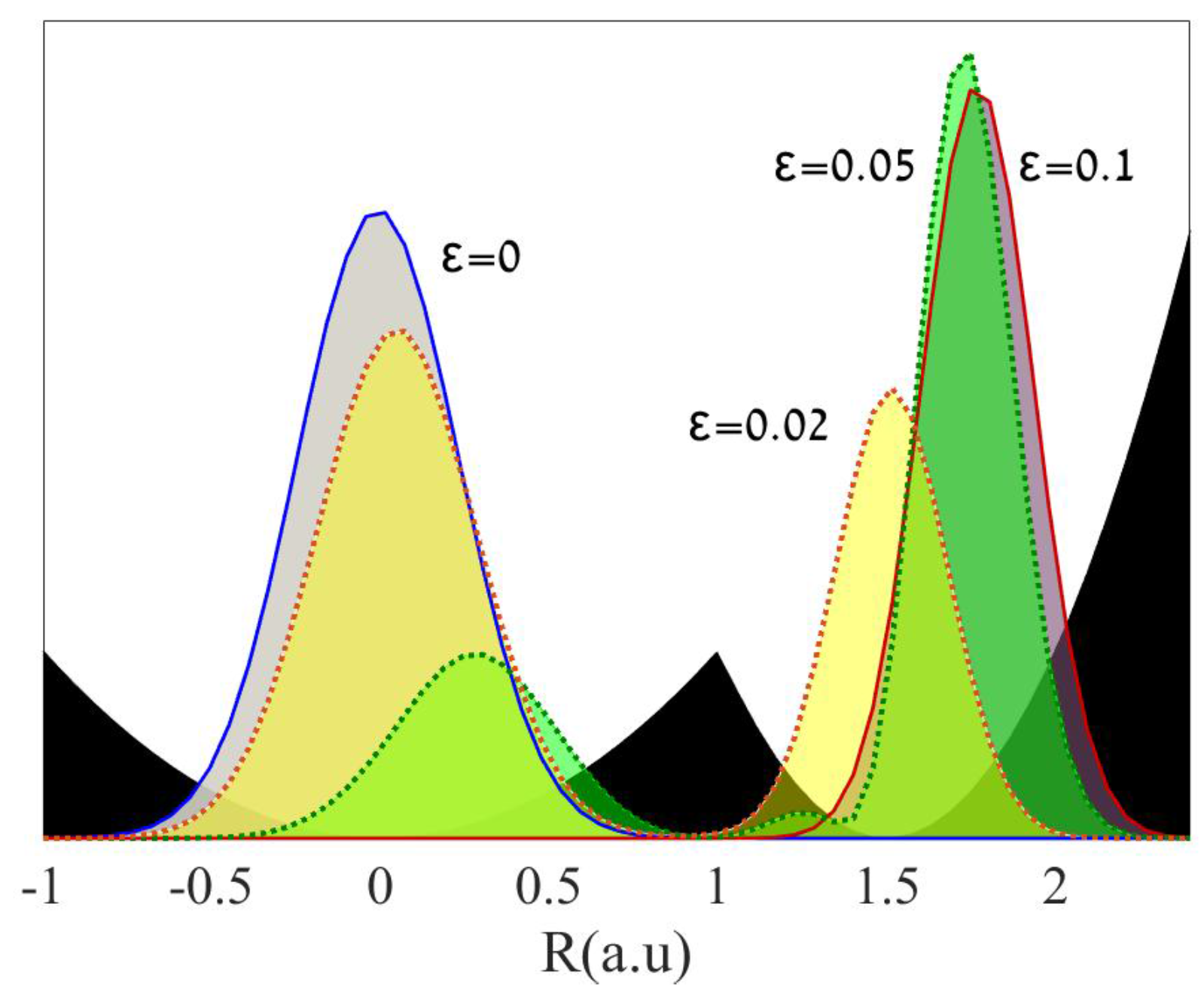
The change in the location of the steady state probability density is shown in
Figure 7 for different driving amplitudes
ϵ. For small
ϵ, the density localizes on the cold potential well, which is wider and has a lower zero point energy. Increasing
ϵ leads to delocalization accompanied by an increase in cooling power. Further increase in driving amplitude localizes the density at the hot side with decreasing cooling power.
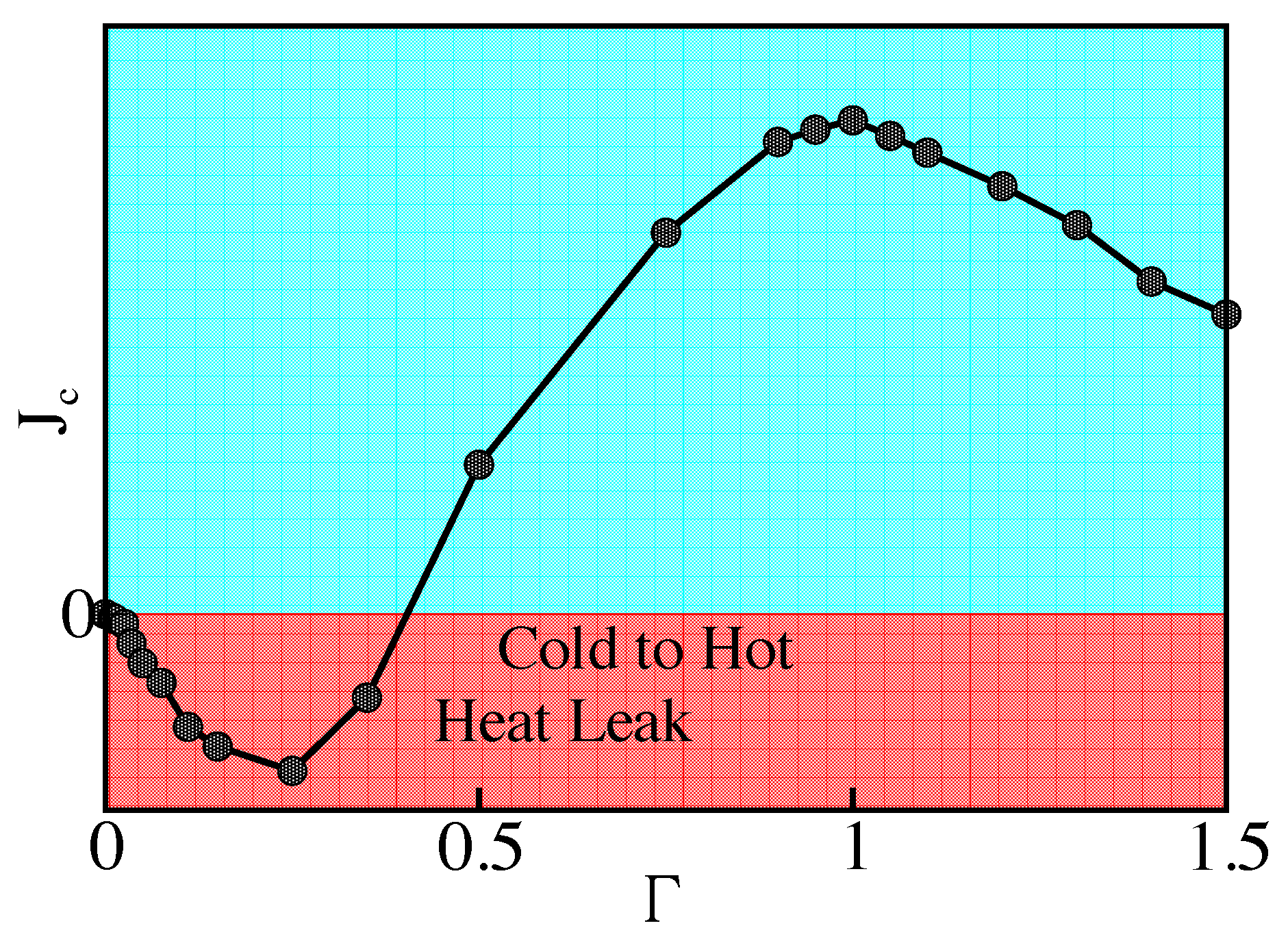
The transition form weak to strong coupling to the baths is demonstrated in
Figure 8. When the coupling parameter Γ is smaller than the driving amplitude
ϵ, no refrigeration is observed. Analysis of the energy currents shows that the heat current to the hot bath
; therefore, the external power is dissipated to the cold bath. We find that the system’s density is localized almost exclusively on the left well. Increasing the coupling leads to a probability density in both wells. At this coupling value, there is a clear maximum in cooling. Further increase of the system–bath coupling leads to a monotonic reduction in the cooling current. This is a manifestation of the strong coupling regime. We find the probability density concentrating on the hot side leading to a loss of coherence, which is essential for the refrigeration.
Continuous quantum devices typically contain coherence in order to perform their task of refrigeration [
39,
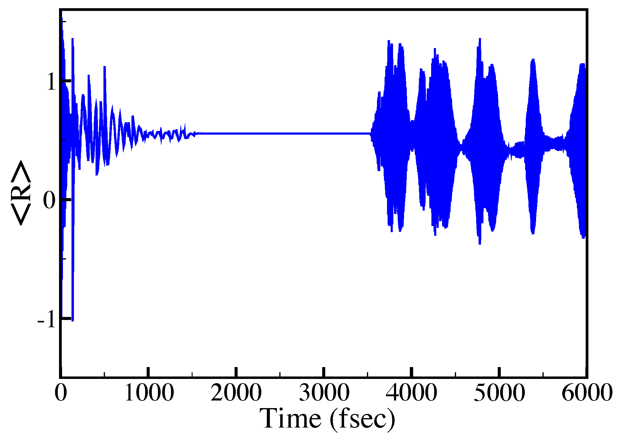
40]. Coherence exists when the state of the system does not commute with its Hamiltonian. To demonstrate this effect, we first let the device reach steady state. This task was achieved in approximately 1500 fsec. We then turned off all external couplings and followed the evolution in time. As a result, the molecule undergoes periodic modulations.
Figure 9 shows the dynamics of the mean position
. The initial dynamics is caused by the approach to steady state. The mean position is biased toward the right bath. At the instant of 3500 fsec, all connections are turned off, ensuing periodic dynamics.
5. Discussion
We studied a quantum molecular device composed of a double well system coupled to a hot and a cold bath. The model is based on a non-Markovian framework where the system and bath are strongly coupled. The device operates as a heat rectifier, facilitating heat transport when the high frequency part of the molecule is coupled to the hot bath. Suppression of heat transport is obtained when the low frequency side is coupled to the hot bath. Recently, there have been experimental realizations of heat rectification [
41,
42,
43]. When an external driving in resonance with the frequency difference of the left and right wells is added, then the device operates as a refrigerator pumping heat from the cold to the hot baths. These features have been observed in properly constructed Markovian models based on the L-GKS equations. A proper construction of L-GKS equations which is consistent with the second law of thermodynamics requires a Floquet analysis, and therefore is limited to periodic driving [
12,
44,
45,
46,
47,
48]. The equations of motion in the SSH approach are independent of the driving field, nevertheless maintaining compliance with the laws of thermodynamics.
The present model allows us to gain insight on the regime of strong driving and strong system–bath coupling. In a continuous device, it is the coherence which is the enabler of operation [
39,
40]. Direct evidence of coherence is that the steady state reduced system state
does not commute with
. This coherence is sensitive to the system–bath coupling parameter Γ. Over-thermalisation causes the system to localize in either the left or the right potential wells. Optimal performance is obtained from a delocalized global state. This interplay explains the dependence of the cooling current
on Γ.
Refrigeration requires a minimum driving amplitude ϵ to overcome the intrinsic heat leak. Overdriving leads to a decrease in . At low ϵ, the system state is localized at the cold side, dissipating power to the cold bath. An increase in ϵ generates a non-local density, supporting flux from the cold to hot bath. Further increase in ϵ localizes the system on the hot side, dissipating power to the hot bath.
The SSH method lends itself to the study of the role of fluctuations in the device currents. We can compare the current in a single realization to the average over many realizations. Due to the size of the Hilbert space in present study (∼10), very few realizations are sufficient to converge the relevant observables. We find that the number of realizations required for convergence is smaller when steady state is reached. A systematic study of fluctuation relations is still required.
To conclude, the stochastic surrogate Hamiltonian model is a viable tool in studying transport and driven transport phenomena in the single device quantum regime.


