Article

Thermoeconomic Coherence: A Methodology for the Analysis and Optimisation of Thermal Systems

by
Antonio Rovira
1,*,
José María Martínez-Val
2 and
Manuel Valdés
2
1
Escuela Técnica Superior de Ingenieros Industriales, Universidad Nacional de Educación a Distancia (UNED), Madrid 28040, Spain
2
Escuela Técnica Superior de Ingenieros Industriales, Universidad Politécnica de Madrid (UPM), Madrid 28006, Spain
*
Author to whom correspondence should be addressed.
Submission received: 29 April 2016 / Revised: 20 June 2016 / Accepted: 30 June 2016 / Published: 5 July 2016
(This article belongs to the Special Issue Thermoeconomics for Energy Efficiency)

Abstract

:
In the field of thermal systems, different approaches and methodologies have been proposed to merge thermodynamics and economics. They are usually referred as thermoeconomic methodologies and their objective is to find the optimum design of the thermal system given a specific objective function. Some thermoeconomic analyses go beyond that objective and attempt to find whether every component of the system is correctly designed or to quantify the inefficiencies of the components in economic terms. This paper takes another step in that direction and presents a new methodology to measure the thermoeconomic coherence of thermal systems, as well as the contribution of each parameter of the system to that coherence. It is based on the equality of marginal costs in the optimum. The methodology establishes a criterion to design coherently the system. Additionally, it may be used to evaluate how much a specific design is far from the optimum, which components are undersized or oversized and to measure the strength of the restrictions of the system. Finally, it may be extended to the analysis of uncertainties of the design process, providing a coherent design and sizing of the components with high uncertainties.

Graphical Abstract

1. Introduction

In the field of thermal systems and, more specifically, in power plants and combined heat and power (CHP) facilities (included trigeneration), different approaches and methodologies have been proposed to merge thermodynamics and economics. These methodologies try to reach a trade-off between thermal efficiency and investment, mainly in the form of minimum generation cost or maximum yearly profit or cash flow.
The common methodology is described, for example, in [1]. It is based on calculating the exploitation costs of the plant, i.e., amortisation cost, fuel costs and operation and maintenance (O&M) costs, and later the generation cost or the profit of the plant. It has been used in many works for the analysis or the optimisation of thermal systems. For example, [2] developed a thermoeconomic tool based on the cash flow estimation that was applied to a combined cycle power plant and [3] proposed an optimisation methodology to minimise the generation cost or to maximise the cash flow using genetic algorithms. Nowadays, the methodology is usually extended to calculate the levelized cost of energy (LCOE) [4] and even the levelized avoided cost of electricity [5], particularly in the field of renewable energy.
Additionally, some methodologies attempt to find whether each component of the facility has been correctly designed or, on the contrary, a wrong design leads to cost inefficiencies. This issue has also been deeply studied, especially by means of the thermoeconomics theory, based on the exergy costing or the exergoeconomic models. These models assign a cost to each exergy flux of the thermal system, allowing the economic evaluation of the plant and finding the contribution of each component to the cost. First studies at this regard were carried out between the 60s and 70s [6,7]. The works of Tsatsaronis and Winhold [8], Frangopoulos [9] and Lozano and Valero [10] as well as the definition of the CGAM [11] and TADEUS (Thermoeconomic Approach to the Diagnosis of Energy Utility System Malfunctions) [12] problems spread out the methodology, which became a powerful tool suitable for any thermal system in general and particularly for CHP systems. These thermoeconomic theories are the basis of a great amount of analyses, optimisations methodologies and even diagnostic tools. The methodology is still being improved taking into account advanced exergy characteristics like the endogenous or exogenous nature of the exergy flux or the avoidable or unavoidable parts of the exergy flux [13] or considering negentropy [14].
Of course, both groups of methodologies are still used. As examples, in [15] a thermoeconomic model is applied to obtain the LCOE of a Kalina Cycle, and in [16] a solar Organic Rankine Cycle is analysed. Besides, exergoeconomics is applied, for example, to new cycle concepts [17], to optimise the off-design operation of a combined cycle [18] or to desalinisation plants [19].
Despite the great amount of works dedicated to find the economic or thermoeconomic optimum, very few of them highlight a result well known in economics, which is that marginal or incremental costs regarding each involved design variable of the system are equal at the optimum. Dechamps [20,21] applies this concept to the optimisations of some parameters of combined cycle gas turbines and heat recovery steam generators. Somehow, this result means that each component has been dimensioned coherently so that all of them contribute with the same weight to achieve the searched objective.
The present work stresses the importance of this result, well known and used in the field of economy but barely used in thermal systems (although the optimization methodologies lead implicitly to it). Marginal costs are defined as the incremental exploitation cost required for a given increment of the product by means of the improvement obtained through the selected path (χ):
M χ = δ E δ P | χ = δ χ ( E ) δ χ ( P ) .
Introducing and formulating explicitly marginal costs in the approach, a new thermoeconomic methodology is proposed, which may be used for the analysis and optimization of the systems as well as to extend it to robustness and uncertainty analyses. Additionally, it allows the definition of a criterion for assessing the design coherence of the thermal system and, particularly, of each component of the system.
The methodology is presented theoretically and applied to a basic example of a closed Brayton cycle. However, it may be applied to complex thermal systems including CHP, and the main guidelines for that purpose are given.

2. Theoretical Background and Conventional Approaches

2.1. General Case: Optimization without Constraints

In the design of thermal power plants, besides thermal efficiency and power rate, two economic results are usually considered: the generation cost (K, in monetary units per kWh) and the yearly cash flow (CF) [1]. Both figures are results that depend on the design of the power plant. Particularly, they are calculated by means of the amortisation cost (A), the fuel cost (F), the operation & maintenance costs (O&M) and the yearly production of the power plant (P). The cash flow also depends on the selling price of the product (V):
K = A + F + O & M P = E P ,
C F = P V ( A + F + O & M ) = P V E = P ( V K ) .
In the above equations, E is the sum of the exploitation costs. All these variables (K, CF, P, E) are functions that depend on the design parameters of the power plant components, which in turn determine variables like the acquisition cost (C) of each component. Besides, these functions also depend on the economic frame considered (interest rate, inflation, escalation rates, expected life, etc.). These dependences may be written as below:
K, E, CF, P f (x1, …, xm).
The set of independent variables xi may be divided into two categories: the first n variables (i from 1 to n) represent the design parameters of the thermal system, while the last mn (i from n+1 to m) represent the economic frame. The design parameters could be any collection of variables that define univocally the system. As mentioned above, they also determine the investment required in each component:
Cjf (x1, …, xn).
The number of components of the thermal system, k, may be lower, equal or higher than the number of degrees of freedom of design parameters, n. If the number of components is higher than the number of the design parameters, the design of one component (or several) is dictated by the others’. Thus, the associated investments must be considered but this component does not contribute to the design of the power plant and it may be obviated in an optimization. If the numbers of components (k) and design parameters (n) are equal, the set of independent variables xi in Equations (4) and (5) may be substituted by the acquisition costs. Finally, if the number of components is lower than the number of design parameters, k variables may represent the investment and the other nk are maintained as design parameters.
The differential form of the functions (4) may be written as below:
d f = i = 1 m f x i d x i = i = 1 m f i d x i .
Besides, considering Equation (1), the marginal cost regarding a specific independent variable of the system (acquisition cost or design parameter) is:
M i = δ E δ P | i = E / x i δ x i P / x i δ x i = E i P i , i = 1... n .
The general optimisation problem is either to minimize the generation cost or to maximize the yearly cash flow (possibly considering environmental externalities like CO2 or other pollutant emissions) given a specific economic frame. If the thermal system is not affected by any constraint, there are n independent variables. Figure 1 depicts the topology of the problem in an example with two independent variables, assuming that the optimum exists.

2.1.1. Minimization of the Generation Cost

Assuming that the minimum generation cost (K*) exists, at that point the partial derivatives regarding any variable are null:
K x i = K i = E i P E P P i P = E i P K * P i P = 0 .
Multiplying Equation (8) by P and considering the definition of the marginal cost:
E i = K * P i M 1 = M 2 = ... = M n = K * .
Equation (9) establishes that, at the design where the generation cost is minimum, all the marginal cost are equal to the generation cost [22]. This result means that the expenditure required improving each parameter or component has a homogeneous contribution to the generation cost. In fact, assuming that the generation cost decreases with the acquisition cost of the components (if they are well designed) the marginal cost is lower than the generation cost, and each improvement contributes to decrease it. In the optimum, where there is not room for further improvements, all the marginal costs equal the generation cost. It may be formulated applying the logarithmic derivative to Equation (2):
1 K K x i = K i K = E i E P i P 0 E i P i E P M i K .
This general optimization case is used to establish the basis of the coherence in the design process: all the marginal costs should be equal. Nevertheless, it is not very representative since in this kind of problems there are usually economies of scale. Thus, the generation cost always decreases with the investment and the optimum without any constraint (fixed total investment, power rate or any other) does not exist.

2.1.2. Maximization of the Yearly Cash Flow

This case is analogous to the previous one but using Equation (3) instead of Equation (2). If the maximum cash flow exists, at that point, the partial derivatives are null and all the marginal costs are equal:
C F x i = C F i = V P i E i = 0 ,
E i = V P i M 1 = M 2 = ... = M k = V .
In this case, the marginal costs take the value of the selling price [22]. As the selling price is presumably higher than the generation cost, the marginal cost at the maximum cash flow design is higher than that obtained at the minimum generation cost. Thus, the maximum cash flow is reached at higher investment rates than the minimum generation cost [23].

2.2. Optimization Subjected to Constraints

The general case described above should be modified in realistic scenarios where there is one or more restrictions to the design. Indeed, a thermal system is always constrained by several restrictions. For example, in the design of a gas turbine, once the compressor has been selected, the nominal pressure ratio of the turbine should fit with the pressure ratio of the compressor. This kind of restrictions may be called internal constraints, since they are not checked at the end of the design process but they are part of the problem formulation. Therefore, they do not require special attention from the designer. Their main consequence is that the number of degrees of freedom is reduced, but Equations (9) and (12) are still correct.
Another kind of restrictions may be, for example, a fixed exhaust gas temperature or a maximum turbine inlet temperature in a gas turbine, the maximum moisture allowed at the exit of a steam turbine, or a fixed power rate or a given maximum total acquisition cost. Constraints may be even applied to a subset of the components of the plant, for example, when a determined commercial gas turbine is used in a project of a combined cycle. These kinds of restrictions may be called external constraints, because they are formulated externally to the problem definition, which only depends on the design variables.
Each restriction may be internal or external depending on the particular problem formulation. For example, in a gas turbine with sequential combustion, the reheating pressure can be internally solved in order to obtain the maximum specific work or to obtain a given exhaust temperature. However, the reheating pressure may be also considered as an independent design parameter that leads to a specific work or exhaust gas temperature that is later externally checked. Hereinafter, only external constraints are considered since internal ones remain hidden. In any case, as it is shown below, the methodology is consistent regardless of whether the restriction is internal or external.
Each external constraint (R) may affect one design variable or a set of design variables, and it is formulated as an additional equation of the system:
R(x1, …, xr, …, xn) = R0.
Therefore, it reduces externally the number of degrees of freedom in a unit: although the number of design parameters does not vary, the constraint determines the selection of one of them once the others have been established.
In general, the problem subjected to a constraint does have an optimum in the restricted domain. For example, for a given power rate, there would be multiple solutions but only one leads to the minimum generation cost. The problem is depicted in Figure 2, similar to Figure 1 but showing the curve that fulfils the constraint.
From the figure, it is observed that the optimum takes place at the tangent point of the curve of the restriction and an iso-curve of the objective function, i.e., the gradient of the iso-curve has null component on the allowed directions established by R. It is important to note that the optimum is not the global optimum, so the restrictions always lead to a worse result (in terms of the objective function) than that obtained considering the unconstrained problem.

2.2.1. Conventional Approach

Assuming that a variable xr can be solved from Equation (13), the differential form of the objective function subjected to the restriction R yields:
df R = i = 1 n f x i d x i = i = 1 , i r n 1 ( f x i + f x r x r x i ) d x i = i = 1 , i r n 1 ( f i + f r x r , i ) d x i .
In the case of the generation cost, the minimum satisfies that the partial derivatives are null:
| R K x i = E i + E r x r , j P E P P i + P r x r , j P = 0 K i R = E i R P E P P i R P = 0 ,
E i R = K * R P i R M 1 R = ... = M n R = K * R .
Therefore, although in general the marginal costs are not equal (since it is not a global minimum), the marginal costs in the domain defined by the restriction (RMi) are equal to the minimum cost in that domain. It is important to note that xr can be a design parameter but also a combination of them, so it represents any direction for varying the design. It can also be noted that, since all the restricted marginal costs are equal, the result of the externally constrained optimization is congruent with the internally constrained one, in which the constraint is intrinsically defined and, as result, all the marginal costs, internally constrained, are equal.
Equations (15) and (16) also highlight that the marginal costs are not defined if the restriction affects the yearly production, since RPi becomes zero. Therefore, this approach is not suitable with such a constraint, which may be a usual restriction if the power rate is fixed. Another singularity arises when the restriction makes the exploitation costs be constant. In such a case, constrained marginal costs are always zero.
This formulation conveys another drawback in order to define a measure of the design coherence. As said before, all the marginal costs are equal at the optimum and coherence should be maximum at this point. But in other design points different from the optimum, marginal costs are different and, moreover, they depend on the variable or direction that has been selected as dependent. For that reason, it can be said that they are not universal, and this is a problem to define a measure of the coherence, that should lay on the design itself regardless of the set of independent variables.

2.2.2. Lagrange Multipliers

Another approach to solve the constrained problem involves the Lagrange multipliers [24,25]. Using Lagrange multipliers, the function to optimize is the Lagrangian. Following with the generation cost minimisation, the Lagrangian (noted as LK if it is applied to the generation cost) considering the restriction R is:
L K = K λ ( R R 0 ) .
In the minimum, the partial derivatives are zero:
{ K i λ R i = E i P K * P i P λ R i = 0 R = R 0 ,
which establishes that the optimum point fulfils the restriction and that both spaces, iso-curves (of generation cost) and restriction, are tangent. Besides, the Lagrange multiplier λ represent the variation of the minimum cost regarding the restriction R. Multiplying the first equation of (18) by P/Pi yields:
M i K * λ P R i P i = 0 ,
M i C = M i λ P R i P i = K * R .
Again, the global marginal costs (Mi) at the optimum are not equal but all the corrected marginal costs (CMi) equal the generation cost. Additionally, the formulation is suitable even at constrained yearly production, and only is undetermined if Pi is null, which only might take place locally (in such case, equal marginal costs are ensured in the nearby of that singular point by Equations (19) and (20)) because otherwise this design parameter is not useful. It is important to note that the corrected marginal cost is not a marginal cost calculated through a specific and allowed direction, but a modification of the marginal cost following the path of the i-th design parameter. This allows CMi to be defined even at constant production. Moreover, taking into account that Ri = Pi, Equation (19) gives additional information and ensures that all the unconstrained marginal costs are equal in all directions, like in the case of the unconstrained optimum, although they are different from the generation cost.
This result suggests that restriction of production is a singular constraint. In fact, increasing production is the natural path to increase the size of the plant. And the same can be said when the restriction makes the exploitation costs constant. If Ri = Ei, then Equation (19) ensures that unconstrained marginal costs are again equal in the optimum. In both cases, the design is quite coherent since it ensures minimum exploitation costs given a yearly production or maximum production given a specific exploitation cost.
As a drawback, this corrected marginal cost based on the Lagrange multipliers is not defined out of the optimum design because the multiplier, λ, is only defined at the optimum. Thus, another approach should be formulated to calculate corrected marginal costs out of the optimum and to let these marginal costs be standard, in the sense of not depending on the set of design parameters selected for the system.

3. Proposed Methodology: Corrected Standardised Marginal Costs and Divergence from the Coherent Design

As it has been shown in previous sections, usual approaches convey several disadvantages to define a coherence criterion, i.e., dependence on the set of variables and definition of the marginal costs in the constrained domain and out of the optimum. In order to solve these drawbacks, marginal costs may be re-defined as it is proposed below. This approach involves three steps: the standardization of marginal costs, the definition of the corrected and standardised marginal costs and the formulation of the divergence from the optimum design.

3.1. Equivalent Standardised Marginal Costs

The problem of standardisation might be overcome if the paths or directions to calculate the marginal costs are those defined by increasing the acquisition cost of each component while the others are constant. The marginal cost regarding an acquisition cost measures the ratio of the incremental exploitation cost to the incremental production when such acquisition cost is increased. However, as discussed previously, using the investments instead of the design parameters may lead to a not completely defined problem. For example, if the number of independent variables were higher than the number of components, once the investments have been selected there would be still some degrees of freedom.
Such standardised directions, which would be universal, are the most convenient but they are not feasible in the cases where the number of components is different to the degrees of freedom.
Another possibility to standardise directions is to find parameters that are common to all thermal systems regardless of the set of variables that allows the calculation of the system, and that do not depend on, for example, the kind of fluid, the pressure or temperature levels or the type of component. These parameters may be a set of exergy fluxes.
Specifically, there are two types of design parameters. One type involves parameters that define some intensive features of the components (pressures, pressure ratios, temperature differences, etc.) and the other type involves extensive parameters (particularly only one, for example, a mass flow rate) which allow the sizing of the components.
The intensive parameters may be replaced by intensive exergy fluxes associated to the involved component. Particularly, if the component exchanges exergy with the environment (for example, in case of compressors, expanders or heat sources or sinks), the incoming or outgoing exergy may be used. On the contrary, when the component is adiabatic and does not exchange mechanical energy (for example, heat exchangers), its internal irreversibility may be used. Finally, if a component has several design parameters associated, the extra parameters may be replaced by extra information related to the irreversibility. For example, the irreversibility of a compressor if the isentropic efficiency is given, or the irreversibility caused by the pressure drop of a stream in a heat exchanger.
Regarding the extensive parameter, it is usually defined by a mass flow rate or by a thermal power. In order to standardise it, the original parameter may be replaced by the power rate supplied by the source that feeds the system, commonly the thermal power at the heat source. At this regard, the exergy content of this thermal power should be avoided to ensure linear independence with the intensive parameters. The power rate of the final products must also be avoided to ensure calculation of the marginal costs associated to those products.
Finally, the specific exergy fluxes that replace the original intensive parameters may be calculated as the exergy flux considered (in power units) divided by the thermal power that feeds the system (also in power units), to ensure the independence of the properties of the fluid.
Using these rules, the standardised marginal costs do not depend on the set of design parameters selected (of varied nature) but on the design point itself. At the optimum, all of them are equal, because none of the allowed directions is preferential or leads to improvements, and make possible comparisons between different types of power plants.

3.2. Corrected Standardised Marginal Costs

Once the standardisation is achieved, the next step is to give an expression for the corrected marginal cost when the problem is constrained. This expression should be valid both in the optimum design and out of the optimum and must be defined even in the cases of constraints of constant production (and non-null at constant exploitation costs).
These requirements may be satisfied if the Lagrange multipliers method is extended to points different from the optimum. Specifically, as it has been said previously, the Lagrange multipliers method considers that the gradient of the iso-curve has null component on the span of allowed directions compatible with the constraints. Thus, in the optimum, the gradient vector (∇K, in the case of the generation cost) is a linear combination of the gradients of the restrictions (∇Rr):
K = r λ r R r K i = r λ r R r , i ,
which is Equation (18) written in vector form.
Conversely, out of the optimum, the gradient of the iso-curve has a component (RK) in the allowed span of directions (because there is room for improvement within that constraint) while the other component is a linear combination of the constraint gradients:
K = R K + r λ r R r K i = R K i + r λ r R r , i .
Additionally, the scalar product of RK and each ∇Rr should be zero because they are perpendicular, so the components of RK and the value of the λr may be calculated with the following system:
{ K i R + r λ r R r , i = K i i K i R R r , i = 0 .
The corrected marginal cost may be defined exactly as in Equation (20). In (22), when the design is the optimum, RKi is zero and this equation is equal to (21). In that case all the equivalent marginal costs are equal to the generation cost. Out of the optimum, equivalent marginal costs are defined thanks to Equation (23) and are not equal due to the existence of RK.

3.3. Divergence from the Coherent Design

In previous sections, the importance of equal marginal costs, constrained or unconstrained, has been highlighted. Also, some standard directions to assess these marginal costs, non-dependent on the set of design variables, have been proposed. Both issues are necessary to define a function that measures the distance or divergence from the optimal design.
Particularly, three features are required for that measurement:
  • It should be congruent for all the possible sets of design parameters of a system (independence of the coordinate system);
  • It should allow the comparison of the coherence of different facilities with independence of the objective function, its value in the optimum and its number of degrees of freedom;
  • The divergence should be zero at the optimum.
These features imply four requirements. The first feature may be fulfilled if the previously defined standardised marginal costs are used. The second one implies two requirements. Firstly, marginal costs should be normalized, in such a way that they vary from 0 to 1. Secondly, the function to assess the distance should be consistent and comparable regardless of the number of independent variables of the thermal system. Finally, the last feature should be addressed searching an appropriate function that reaches a local extreme when all variables are equal. Two possibilities are either a Cartesian distance or an entropy-like function.
In fact, a suitable function that fulfils these four requirements is the entropy-cross divergence. This function is commonly used to measure divergences between two probability distributions [26]. Somehow, it provides a value that quantifies the information managed to use one probability distribution instead another previous one.
The marginal costs may be normalized as below:
d i = M i 2 C M i 2 C ,
where CMi are the corrected marginal costs described in Section 3.2. Thus, the sum of di is the unit:
i = 1 n d i = 1 .
At the optimum, all the normalised marginal costs are equal and take the value of 1/n.
The divergence to the most coherent design (the optimum), in which all the marginal cost are equal, is calculated by an entropy-cross function and measures the difference between the actual distribution of normalized marginal costs (a given set of di) and the optimum one (all normalized marginal costs equal to 1/n):
D = i = 1 n d i log ( d i / d o p t i m u m , i ) = i = 1 n d i log ( d i n ) .
Such function, subjected to the restriction (26), is minimum and takes the value of zero when all di equal 1/n, and increases as one or several di increase or decrease getting different from the others. Additionally, it ensures the homogeneity of the values for different systems with different amount of degrees of freedom n (a Cartesian distance does not achieve this homogeneity). Some examples of this homogeneity are shown in the appendix.
This measure is suitable but does not consider that all the corrected marginal costs are equal to the generation cost (or to the selling price if the cash flow is maximised). To take into account that effect (and following with the generation cost minimization), the summation can be extended including an additional term that considers the generation cost. Moreover, to guarantee the homogeneity in different systems, the additional term should be weighted with a factor n. Thus, the normalized marginal costs and divergence become:
d i = M i 2 C M i 2 C + n K 2 ,
D = n K log ( K 2 n ) + i = 1 n d i log ( d i 2 n ) .
Therefore, when the design is optimum, the divergence of coherence D is null. Divergences different from zero indicate that either the design is not the optimum (because it has been established taking wrong decisions) or that there are some restrictions or information that justify such divergence (but they have not been accounted for in the analysis). Also, the higher the divergence, the lower the design coherence, since some marginal costs are quite different one to the others, and there is room for improving the system.
The divergence can also be used to measure how strong a constraint is. In fact, if the unconstrained marginal costs are used instead the corrected ones, the new divergence is higher and the difference between both ones gives the strength of the constraint.
Finally, the divergence of each parameter may be assessed with the following equation:
D i = d i log ( d i 2 n ) K log ( K 2 n ) ,
which is useful if the associated marginal cost is positive. When this divergence is positive, then the marginal cost is higher than the cost and the parameter should be relaxed, and conversely. Besides, if the marginal cost is negative, the design is very far from the optimum whatever the value of Di.

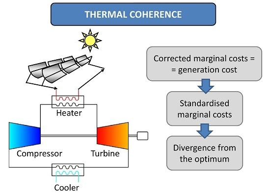
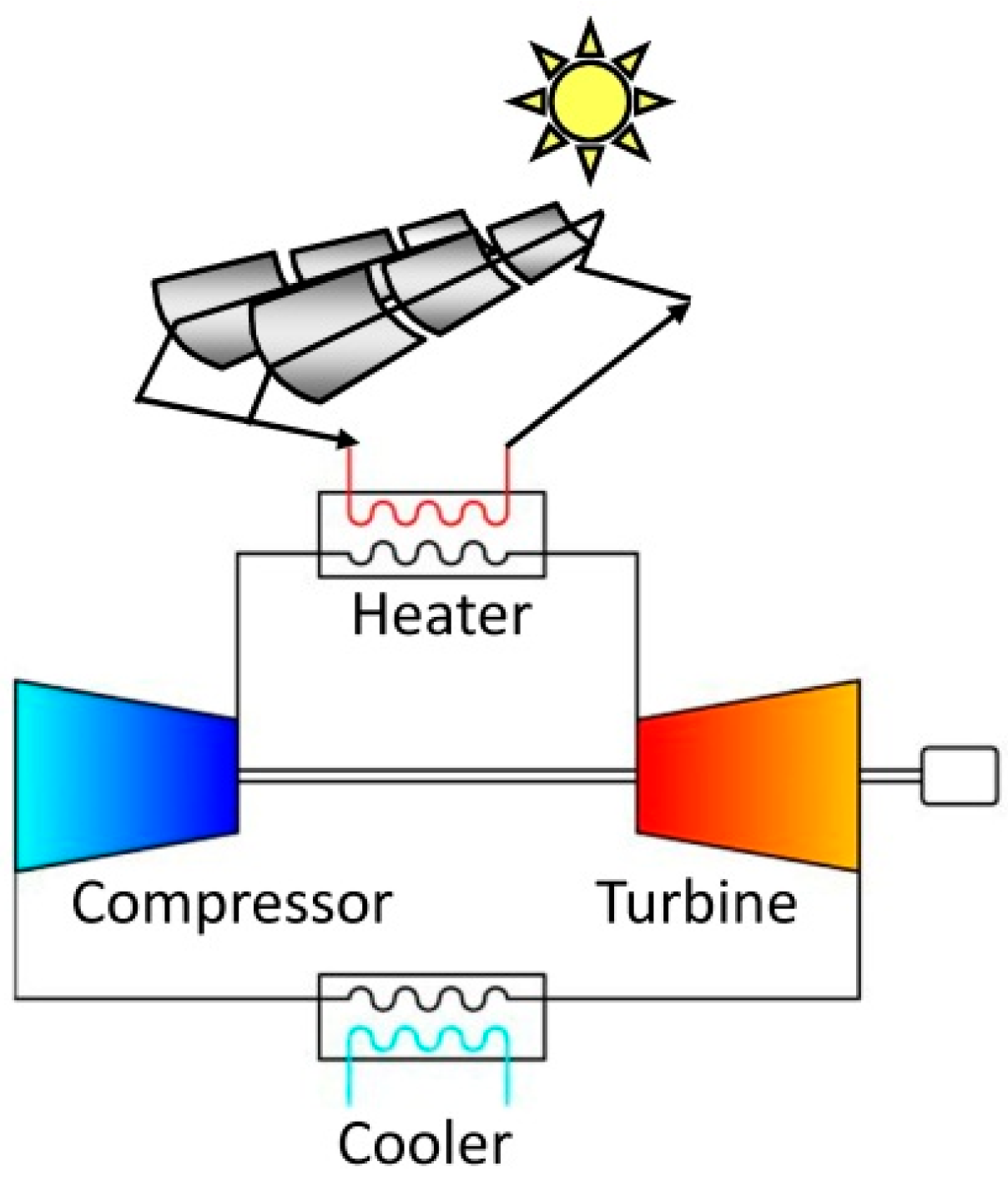
4. Application Example: Coherence in a Solar Gas Turbine

Let us consider a hypothetical solar gas turbine following a closed Brayton cycle as illustrated in Figure 3. Nowadays, solar gas turbines are uncommon systems that have been developed only in research projects. This is an advantage for the present work since the objective of the paper is to present the proposed methodology without focusing on a particular system optimization or discussing the results obtained for a specific power plant (that should be done in future works). Moreover, the choice of a solar gas turbine as an example provides two additional advantages. Firstly, the exploitation costs only depend on the total investment because there is not any expenditure associated to the fuel cost, which are part of the exploitation costs in conventional power plants (neglecting O&M costs). Thus, the effect of constant exploitation costs commented in Section 2.2.1 and Section 2.2.2 can be assessed. Secondly, as a non-conventional system, its design presents some uncertainties that may affect the specific design of the components and the whole power plant. This issue is analysed in Section 5.1, where the methodology is adapted to consider uncertainties.
A possible set of design parameters to define the solar gas turbine are the pressure ratio, the effectiveness of the heater and the cooler, the mass flow rate and the maximum temperature at the solar field. Note that more design variables might have been chosen, like the isentropic efficiencies of the turbomachinery or the pressure drops in the heat exchangers. However, such technological parameters have been maintained constant in order to simplify the analysis (an isentropic efficiency of 90% for the turbomachinery and null pressure drops have been considered).
The performance of the thermal system may obtained by applying mass and energy balances to each component. The yearly production may be estimated assuming, for example, 4000 equivalent hours working at full load. Finally, the exploitation costs may be calculated using a costing model for each component and a given economic frame (for example, an interest rate of and a life that lead to a capital recovery factor of 15).
As the objective of this section is to give a qualitative application example, actual and accurate costing models are not required. Indeed, comprehensive optimisation of thermal systems requires more data than those used in the example. For that reason, some arbitrary costing models in arbitrary monetary units (mu) are proposed, qualitatively plausible but without quantitative accuracy. The models are shown in Table 1. From the equations of the table, it may be observed that the costing model establishes economy of scale, since specific investment (ratio of acquisition cost to mass flow or thermal power) decreases with the size of the system (determined by the mass flow rate or supplied thermal power).
Table 2 shows an arbitrary selection of the five design parameters together with the exploitation cost, yearly production, generation cost and the marginal cost regarding the design parameters. Such design may serve as the base case for further comparisons. As observed, the marginal costs are different one to the others, so this arbitrary design is not the optimum. Furthermore, in this case, the global optimum of the system does not exist because of the economy of scale.
According to Section 3.1, marginal costs should be assessed through a set of standardised paths. In the case of the proposed solar gas turbine, the following parameters are considered:
  • The pressure ratio (intensive parameter) is replaced by the ratio of the compressor power to the thermal power supplied to the system ( W ˙ C / Q ˙ ).
  • The effectiveness (intensive parameter) of the heater and cooler are replaced by the ratio of their irreversibility to the thermal power supplied to the system ( I ˙ / Q ˙ ).
  • The maximum temperature of the solar field (intensive parameter) is replaced by the ratio of the exergy content of the thermal power to the supplied thermal power ( E ˙ Q / Q ˙ ).
  • The mass flow (the extensive parameter) is replaced by the thermal power supplied to the system ( Q ˙ ).
In order to assess the partial derivatives required to evaluate the gradients considering the standardized parameters (fj,standardized) instead the original ones (fi,original), the Jacobian matrix that contains the derivatives of these standardized parameters (yj) regarding the original ones (xi) should be assessed. The inverse of this Jacobian matrix gives the derivatives of the original parameters regarding the standardized ones, and any other derivative may be calculated as below:
f j , standardized = i f i , o r i g i n a l x i y j ,
For the solar gas turbine considered, four constrained cases have been selected to illustrate the value of the different marginal costs. The cases are (1) fixed investment–equal to the base case; (2) fixed production–equal to the base case; (3) fixed production and turbine exhaust temperature–both equal to the base case; and (4) fixed production and turbine inlet temperature–again both equal to the base case.
Table 3 shows the results of the main parameters of the solar gas turbine in all cases, including the base case for comparative purposes. It can be observed that when the investment is fixed the exploitation cost is constant too because, as mentioned, in this particular system there is not any expenditure associated to the fuel cost.
Table 4 shows the unconstrained marginal costs regarding the original design parameters and the standardised and unconstrained marginal costs in all the considered cases. As expected, the marginal costs regarding the design parameters are only the same in the optimisations of constant investment (because it leads to constant exploitation costs) and constant production. In the other cases, they are different because the design is not the optimum in that domain (unrestricted).
Also, for the cases of constant production and constant exploitation costs, all standardised marginal costs are the same as those regarding the design parameters because, as said previously, in these cases equality of marginal cost takes also place at the unconstrained domain, and none of the possible directions is preferred.
According to Section 3.2, marginal costs should be corrected taking into account the constraints of the problem. Table 5 shows these corrected standardized marginal costs for each optimized case, those corresponding to the base case in each respective constrained domain and the value of the lambdas. As observed, the corrected marginal costs in the optimized cases are equal to the generation cost. Conversely, those of the base case are different and, even, some of them are negative, which means that the design and, particularly, the value of the corresponding parameter are quite far from the optimum one.
Finally, once the corrected standardised marginal costs are obtained, the divergence from the coherent design may be assessed with Equations (29) and (30) (Section 3.3).
Table 6 shows the divergence D of the different cases considered for the example (base case and optimisations) considering the unconstrained domain and the divergence of each parameter (Di). The divergence is not zero in any case because none of the design is the optimum in the unconstrained domain. However, it is close to zero in the cases of constant investment (constant exploitation cost) and constant production because all marginal costs are equal, although different from the generation cost. In those cases, the divergence measures the strength of the restriction. The value of the divergences gets higher in the base case and in the cases of constant production and constant turbine exhaust temperature or turbine inlet temperature. In the base case, it happens because the design is not an optimum. In the other cases, the marginal costs used are the unconstrained ones, so the value of the divergence measures the strength of the restriction.
Table 7 shows the divergence of the optimised designs and the base case at each constrained domain through the corrected marginal costs. As observed, the divergences for the optimised cases are roughly zero. Conversely, the base case is far from the coherent design at the constrained domain.

5. Extension of the Methodology to Robustness and Uncertainty Analysis and Combined Heat and Power

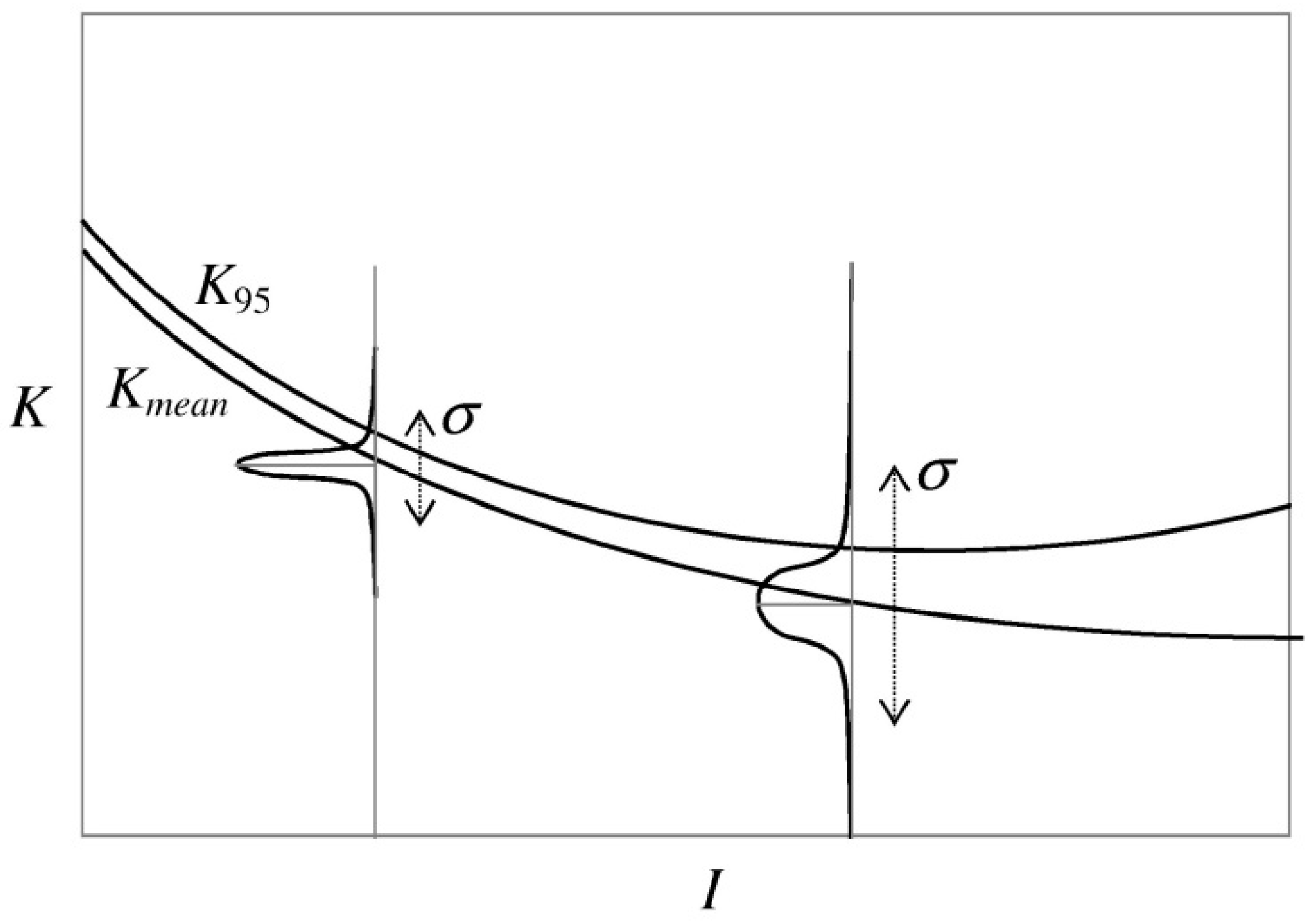
5.1. Robustness and Uncertainty: Optimization in Economy of Scales

The methodology shown in previous sections has been developed for a given economic frame with all the variables and functions well defined in a deterministic way. However, thermal systems are facilities that work during many years, so the estimation of the economic frame or any other variable (performance, ambient conditions, etc.) might not be accurate. Likewise, some of the components may be innovative and not proven in depth. Therefore, the problem may have a certain degree of uncertainty that should be considered. A possibility to take that uncertainty into account is to perform sensitivity analyses to the most relevant variables, comparing the results under different possible frames.
Of course, the uncertainties may affect the selection of the optimum design point. Besides, they may also introduce some questions about how large the power plant should be taking into account the risk in predicting the frame, or how much an innovative component should be undersized or oversized to guarantee a coherent design minimizing risks. These aspects may lead to the existence of a coherent optimum even in unconstrained problems regarding the size or investment where, without considering uncertainties, there are economies of scale.
These questions are not usually evaluated quantitatively during the design process. However, the presented methodology can deal with them by means of a slight modification of the marginal costs.
Specifically, the problem defined by the functions of Equation (4) can depend on design parameters xi that either are not deterministic or their influence on the functions have some uncertainty. With such premises, results like the generation cost (K), the cash flow (CF), the exploitation cost (E) or the yearly production (P) are of probabilistic nature and they follow certain density function. Whatever the density function, it is possible to define a variability of the results through the variance, σ, and a selected confidence level for the result. For example, given a set of variables xi it is possible to obtain a result, for example of the generation cost, which ensures with a confidence level of 95% that the actual cost is below that value. Therefore, it is possible to represent the curve of the generation cost with a confidence level of 95%.
Figure 4 shows that curve together with the mean or expected value of the distribution (it is assumed for comparative purposes that, in the limit, it agrees with the deterministic analysis value). Both are represented versus the total investment, which depends only on the size of the plant. The curve has been represented assuming that the variance σ increases with the plant size:
σ ( x 1 , ... , x n ) P i | i = 1... k > 0 .
Increasing variances with size (or production if the components are well designed) is a plausible hypothesis, since all magnitudes increases with size. However, this might not necessarily be true.
According to Figure 4 and for increasing variances with investment and production, the minimum generation cost at a confidence level is obtained at lower sizes than that of the deterministic analysis (and vice-versa). Therefore, under uncertainties, the sizing of the equipment should be conservative.
For a given density function, the expected generation cost and the generation cost at a confidence level are related as below:
K95 = K +A·σ,
where A is a characteristic of the density function.
Minimising K95:
K 95 x i = K 95 , i = K x i + A σ x i = K i + A σ i = 0 ,
Taking into account Equation (2) and considering the definition of the marginal costs (Equation (1)):
E i P K P i P + A σ i = 0 ,
M i + A P σ i P i = M i + A P δ i σ δ i P = K ,
thus, another corrected marginal cost may be defined as below:
M σ = M i + A P σ P , i = K .
For the cash flow, where FC95 = FCA·σ, Equation (33) becomes:
F C 95 x i = F C 95 , i = F C x i A σ x i = F C i A σ i = 0 ,
considering Equation (3) yields:
V P i E i A σ i = 0 .
If Equation (38) is divided by Pi and taking into account the definition of marginal cost:
M i + A σ i P i = M i + A δ i σ δ i P = V ,
which allows the definition of the corrected marginal cost:
M σ = M i + A σ P , i = V .
Equations (36) and (40) indicate that if all the variations of variance are equal in all directions, σP,i, the marginal costs are equal although lower than those obtained in a deterministic optimization. Thus, the coherent design is reached at the conservative side of sizing (and the contrary if variances decrease). The level of information or the strength of the restriction given by the probabilistic approach may be again calculated by comparing the thermal coherence using the corrected and unconstrained marginal costs, taking the uncertainty as a constraint-like condition.
Besides, if a variance increases at higher rate than the others, the coherent marginal cost should be lower, so that component should be even more conservative.
Finally, in both cases (balanced or unbalanced variance variations and increasing with production), the coherent designs lead to undersize the affected components and to worse economic results than in a deterministic case without uncertainties. Additionally, if not all the variances decrease homogeneously, the coherent design is farther than the deterministic optimum, and that situation should not be obviated.
Innovative technologies and components can have higher uncertainties than conventional ones. Taking into account the coherence criteria, the investment in those components should not be disproportionately high regarding the others’. This conclusion, which might be mitigated by incentives, should be taken as a prudence decision, and not as a disincentive for installing new clean technologies.
There are two possibilities to apply the coherence criterion considering uncertainties. Firstly, a probabilistic study may be carried out in order to know the density distribution of both the design variables and the results. Another approach is to introduce a coefficient in the constrained marginal costs that acts as a safety factor:
M σ , i R = M m , i R = ( 1 + m i ) M i R .
This formulation is simpler than the probabilistic studies but requires further studies to quantify the value of the coefficient m, which is characteristic of each problem.
In the case of the solar gas turbine shown as an example, two optimisation cases are presented to illustrate the effect of an uncertainty in the yearly production. In one case the variance increases with its own production (equal for all the design parameters) without any constraint, and in the other it increases only with the maximum temperature of the solar field, that simulates an uncertainty in an innovative component, and considers a fixed production equal to the base case. Table 8 shows the results obtained for these optimisations.
It may be observed that in the case of a homogenous variation of the variance there is an optimum despite the economies of scale, as illustrated in Figure 4. All the marginal costs are equal due to the homogeneous variation of the variance but the divergence is not null because marginal costs are different from the generation cost. Finally, all the divergences of the parameters are negative, which means that the parameters are under-sized if they are compared to the deterministic unconstrained case. It is important to note that the divergence has been calculated with the marginal costs and not the corrected ones. If they are corrected with the value of m as in Equation (41), the divergences are null and the marginal costs equal the generation cost.
In the case of a variation of the variance of the production with the maximum temperature, all the marginal costs are equal except for that of the maximum temperature, which takes a value lower than the others’. In fact, the optimisation is similar to a case of maximum temperature constrain. The results are worse than the obtained in the case of the constant yearly production. Finally, the divergence to the optimum is not null and the divergence of each parameter is negative, especially that of the maximum temperature.

5.2. Combined Heat and Power

The objective of this section is to give some guidelines to extend the proposed methodology to CHP systems. The thermal requirements of CHP are quite varied and the casuistic of the designs may be high, so further studies to fully develop the methodology should be performed in the future.
Particularly, CHP systems are facilities designed to produce two or more products, one of them is mechanical power and the others are thermal power (for heating and/or cooling). As the exploitation costs are common for all the products, some extra information is required to evaluate the cost of each product or the profit of the power plant.
For example, assuming that there are two products (i.e., power, P1, and heat, P2), the most simple case is that in which both selling prices (V1, V2) are known. In this case, the thermoeconomic objective is to maximise the yearly profit or cash flow of the power plant:
C F = P 1 V 1 + P 2 V 2 E .
In the optimum, the derivatives regarding any variable are null, thus:
P 1 , i V 1 + P 2 , i V 2 = E i .
As the marginal cost of each product is the incremental exploitation cost divided by the incremental production:
V 1 / M 1 , i + V 2 / M 2 , i = 1 M 1 , i ( 1 V 2 / M 2 , i ) = V 1 .
This expression is analogue to that used to calculate the corrected marginal costs, and indicates that this corrected marginal cost is the same for all variables in the optimum and equal to the selling price.
Another possible simple case is that in which the selling price of a product (V2) is known and the cost of the other (K1) is calculated. In such case, the minimum price at which the product should be sold is:
K 1 = E P 2 V 2 P 1 .
Minimising that generation cost and calculating the marginal cost as before yields:
E i P 2 , i V 2 P 1 K 1 P 1 , i P 1 = 0 ,
M 1 , i ( 1 V 2 / M 2 , i ) = K 1 .
The expression above is again analogous to the previous ones and makes all the corrected marginal costs equal to the generation cost at the optimum.
Finally, the above cases may be extended to that in which none of the selling prices is known and the cash flow or the generation cost of a product is optimised. In those cases, some extra information is required. For example, if one of the products is considered as the main one, its generation cost may be estimated considering a system without cogeneration. Once that cost is estimated, the other may be calculated as the incremental cost (K1) in the new system (Equation (42) replacing V2 by the cost of the main product, K2), and this incremental cost can be minimised. In this case, the expression is equal to Equation (44) changing V2 by the cost of the main product, K2.
Another possibility is to know information about the demand curve of the products, in the form of how the selling price varies as function of the production. In such case, one (V2) or both (V1, V2) selling prices are function on the respective productions, V1 (P1) and V2 (P2), and Equations (44) and (47) become:
V 1 = M 1 , i ( 1 V 2 V ' 2 P 2 , i M 2 , i ) + V ' 1 P 1 , i ,
K 1 = M 1 , i ( 1 V 2 V ' 2 P 2 , i M 2 , i ) ,
which have the same form as the previous ones.

6. Conclusions

A new methodology to measure the thermoeconomic coherence of thermal systems has been presented and applied to a solar gas turbine as an example. Based on the equality of marginal costs in the optimum, the methodology establishes a criterion to design coherently the system. Besides that, it provides a measure to assess the contribution of each parameter of the system to that coherence.
The basic criterion for the coherent design lies on the equality of all marginal costs in the optimum design point. However, the marginal cost should be conveniently defined and used to make the methodology robust and comparable for any thermal system, even when the number of degrees of freedom are different or the system is constrained by any kind of restriction. Particularly, the set of paths at which the marginal costs should be evaluated has been proposed, the expressions for correcting marginal costs have been given and a function to measure the divergence to the optimum design has been formulated.
The proposed methodology may be used to evaluate how much a specific design is far from the optimum, which components are undersized or oversized and to measure the strength of the restrictions of the system. Finally, it may be extended to the analysis of uncertainties of the design process, providing a coherent design and sizing of the components with highest uncertainty. Despite it has been applied to a power plant dedicated to electricity production, some guidelines have been given to extend it to combined heat and power systems.

Acknowledgments

Authors acknowledge the financial support of the Spanish Ministry of Economy and Competitiveness to the ENE2012-37950-C02-01/ENE2012-37950-C02-02 and ENE2015-70515-C2-1-R/ENE2015-70515-C2-2-R research projects.

Author Contributions

All authors contributed to this work by collaboration. Antonio Rovira is the first author who proposed specific objectives of the methodology, developed the mathematical formulation and helped in establishing the framework of the paper. José María Martínez-Val defined the ambition of the paper: the thermal coherence linked to an entropic formulation, and helped in preparing the specific objectives. Manuel Valdés helped, debugged and incorporated valuable suggestions regarding thermoeconomics, the mathematical formulation and writing the paper. All authors have read and approved the final manuscript.

Conflicts of Interest

The authors declare no conflict of interest.

Nomenclature

The following nomenclature and abbreviations are used in this manuscript:
Acronyms
CGAMCHP problem defined in [11]
CHPCombined heat and power
LCOELevelized cost of energy
MuMonetary units
O&MOperation & maintenance cost
TADEUSThermoeconomic Approach to the Diagnosis of Energy Utility System Malfunctions [12]
Symbols
AAmortisation cost (monetary units, mu); Constant of the probability distributions
CAcquisition cost (mu)
CFCash flow (mu)
dNormalized marginal cost (-)
DDivergence (-)
EExploitation cost (mu)
E ˙ Q Exergy content of the thermal power (W)
fgeneric function
FFuel cost (mu)
I ˙ Irreversibility (W)
ItotalTotal investment (mu)
KGeneration cost (mu·J−1)
msafety coefficient, number of variables including the economic frame
m ˙ Mass flow rate (kg·s−1)
MMarginal cost (mu·J−1)
nNumber of degrees of freedom
PYearly production of the plant (J)
Q ˙ Thermal power rate at the heat source (W)
RRestriction
TitTurbine inlet temperature (K)
TexhTurbine exhaust temperature (K)
TmaxMaximum temperature of the solar field (K)
UAProduct of the overall heat transfer coefficient and the heat exchange area (W·K−1)
VSelling price of the product (mu·J−1)
W ˙ C Compressor power (W)
xOriginal design parameters
yStandardized variables
Greek letters
Δincrement
εHeat exchanger effectiveness (-)
ηthermal efficiency (-)
ΛLagrange multiplier
Πpressure ratio (-)
ΣVariance
Subscripts
coolCooler
compCompressor
GTGas turbine
heatHeater
solarSolar field
turbTurbine

Appendix

In this appendix the independence of the divergence to the optimum design regarding the number of design parameters is shown.
Let us consider two different thermal systems with different number of degrees of freedom (n). And let us consider that, for example, in both systems a half of normalized marginal cost takes a value d0 and the other half a value of y times d0. The divergences in both cases are:
D = i = 1 n / 2 d i · log ( d i · n ) + i = n / 2 + 1 n d i · log ( d i · n ) = n 2 d 0 · log ( d 0 · n ) + n 2 y d 0 · log ( y d 0 · n ) .
Considering that the sum of di is 1/n (Equation (26)):
i = 1 n d i = n 2 d 0 + n 2 y d 0 = 1 d 0 = 2 n ( 1 + y ) .
Equation (A1) becomes:
D = 1 ( 1 + y ) log ( 2 ( 1 + y ) ) + y ( 1 + y ) log ( 2 y ( 1 + y ) ) .
That does not depend on the number of degrees of freedom, n.
Of course, the highest divergence occurs when a normalized marginal cost is the unit. It that case, the higher n, the higher the divergence, that is logical since the design is also more unbalanced:
D = i = 1 n d i log ( d i n ) = log ( n ) .
However, the comparable cases for two thermal systems that have different degrees of freedom are, assuming for example that a n is double than the other, those in which one has a normalized marginal cost of unit and the other two normalized marginal cost are 0.5, because the proportion of high marginal costs and low marginal costs is the same. In such case the divergences are equal:
D = log ( n ) = 0.5 log ( 0.5 ( 2 n ) ) + 0.5 log ( 0.5 ( 2 n ) ) .

References

  1. Bejan, A.; Tsatsaronis, G.; Moran, M. Thermal design and optimization, 1st ed.; John Wiley & sons: Hoboken, NJ, USA, 1996. [Google Scholar]
  2. Attala, L.; Facchini, B.; Ferrara, G. Thermoeconomic Optimization Method as Design Tool in Gas-Steam Combined Plant Realization. Energy Convers. Manag. 2001, 42, 2163–2172. [Google Scholar] [CrossRef]
  3. Valdés, M.; Durán, M.D.; Rovira, A. Thermoeconomic optimization of combined cycle gas turbine using genetic algorithms. Appl. Therm. Eng. 2003, 23, 2169–2182. [Google Scholar] [CrossRef]
  4. International Renewable Energy Agency. Available online: http://www.irena.org/documentdownloads/publications/re_technologies_cost_analysis-csp.pdf (assessed on 1 July 2016).
  5. Energy Information Administration. Available online: https://www.eia.gov/forecasts/aeo/pdf/electricity_generation.pdf (assessed on 1 July 2016).
  6. Evans, R.B. A Contribution to the Theory of Thermoeconomics. Master’s Thesis, University of California, Los Angeles, CA, USA, 1961. [Google Scholar]
  7. El-Sayed, Y.M.; Evans, R.B. Thermoeconomics and the Design of Heat Systems. Trans. ASME J. Eng. Power 1970, 92, 27–34. [Google Scholar] [CrossRef]
  8. Tsatsaronis, G.; Winhold, M. Exergoeconomic Analysis and Evaluation of Energy Conversion Plants—I. A New General Methodology. Energy 1985, 10, 69–80. [Google Scholar] [CrossRef]
  9. Frangopoulos, C.A. Thermo-Economic Functional Analysis and Optimization. Energy 1987, 12, 563–571. [Google Scholar] [CrossRef]
  10. Lozano, M.A.; Valero, A. Theory of the Exergetic Cost. Energy 1993, 18, 39–60. [Google Scholar] [CrossRef]
  11. Valero, A.; Lozano, M.A.; Serra, L.; Tsatsaronis, G.; Pisa, J.; Frangopoulos, C.A.; von Spakovsky, M. CGAM Problem: Definition and Conventional Solution. Energy 1994, 19, 279–286. [Google Scholar] [CrossRef]
  12. Valero, A.; Correas, L.; Zaleta, A.; Lazzaretto, A.; Verda, V.; Reini, M.; Rangel, V. On the thermoeconomic approach to the diagnosis of energy system malfunctions—Part 1: the TADEUS problem. Energy 2004, 29, 1875–1887. [Google Scholar] [CrossRef]
  13. Petrakopoulou, F.; Tsatsaronis, G.; Morosuk, T.; Carassai, A. Advanced Exergoeconomic Analysis Applied to a Complex Energy Conversion System. J. Eng. Gas Turbines Power 2012, 134. [Google Scholar] [CrossRef]
  14. Li, H.; Chen, J.; Sheng, D.; Li, W. The improved distribution method of negentropy and performance evaluation of CCPPs based on the structure theory of thermoeconomics. Appl. Therm. Eng. 2016, 96, 64–75. [Google Scholar] [CrossRef]
  15. Modi, A.; Kærn, M.R.; Andreasen, J.G.; Haglind, F. Thermoeconomic optimization of a Kalina cycle for a central receiver concentrating solar power plant. Energy Convers. Manage. 2016, 115, 276–287. [Google Scholar] [CrossRef] [Green Version]
  16. Baral, S.; Kim, D.; Yun, E.; Kim, K.C. Experimental and Thermoeconomic Analysis of Small-Scale Solar Organic Rankine Cycle (SORC) System. Entropy 2015, 17, 2039–2061. [Google Scholar] [CrossRef]
  17. Ozcan, H.; Dincer, I. Exergoeconomic optimization of a new four-step magnesiumechlorine cycle. Int. J. Hydrog. Energy. in press. [CrossRef]
  18. Keshavarzian, S.; Gardumi, F.; Rocco, M.V.; Colombo, E. Off-Design Modeling of Natural Gas Combined Cycle Power Plants: An Order Reduction by Means of Thermoeconomic Input–Output Analysis. Entropy 2016, 18. [Google Scholar] [CrossRef] [Green Version]
  19. Piacentino, A. Application of advanced thermodynamics, thermoeconomics and exergy costing to a Multiple Effect Distillation plant: In-depth analysis of cost formation process. Desalination 2015, 371, 88–103. [Google Scholar] [CrossRef]
  20. Dechamps, P.J. Incremental cost optimization of Heat Recovery Steam Generators; 95-CTP-101; The American Society of Mechanical Engineers: New York, NY, USA, 1995. [Google Scholar]
  21. Dechamps, P.J. The optimization of combined cycle HRSGs as a function of the plant load duty. In Proceedings of the ASME 1996 International Gas Turbine and Aeroengine Congress and Exhibition, Birmingham, UK, 10–13 June 1996.
  22. Kirschen, D.; Strbac, G. Fundamentals of Power System Economics; John Wiley & sons: Hoboken, NJ, USA, 2004. [Google Scholar]
  23. Valdés, M.; Rovira, A.; Durán, M.D. Influence of the heat recovery steam generator design parameters on the thermoeconomic performances of combined cycle gas turbine power plants. Int. J. Energy Res. 2004, 28, 1243–1254. [Google Scholar] [CrossRef]
  24. Stoecker, W.F. Design of Thermal Systems, 3rd ed.; MacGraw-Hill Book Company: New York, NY, USA, 1989. [Google Scholar]
  25. Jaluria, Y. Design and Optimization of Thermal Systems, 2nd ed.; CRC Press: Boca Raton, FL, USA, 2008. [Google Scholar]
  26. Shore, J.E.; Johnson, R.W. Axiomatic Derivation of the Principle of Maximum Entropy and the Principle of Minimum Cross-Entropy. IEEE Trans. Inform. 1980, 26, 26–37. [Google Scholar] [CrossRef]
  27. Zare, V.; Mahmoudi, S.M.S.; Yari, M. An exergoeconomic investigation of waste heat recovery from the Gas Turbine-Modular Helium Reactor (GT-MHR) employing an ammonia—water power/cooling cycle. Energy 2013, 61, 397–409. [Google Scholar] [CrossRef]
  28. Ghaebi, H.; Amidpour, M.; Karimkashi, S.; Rezayan, O. Energy, exergy and thermoeconomic analysis of a combined cooling, heating and power (CCHP) system with gas turbine prime mover. Int. J. Energy Res. 2011, 35, 697–709. [Google Scholar] [CrossRef]
  29. Rovira, A.; Barbero, R.; Montes, M.J.; Abbas, R.; Varela, F. Analysis and comparison of Integrated Solar Combined Cycles using parabolic troughs and linear Fresnel reflectors as concentrating systems. Appl. Energy 2016, 162, 990–1000. [Google Scholar] [CrossRef]
Figure 1. Optimum of the objective function.
Entropy 18 00250 g001
Figure 2. Optimum of the objective function with a constraint.
Entropy 18 00250 g002
Figure 3. Closed Brayton cycle.
Entropy 18 00250 g003
Figure 4. Expected or mean generation cost and cost at a 95% confidence level.
Entropy 18 00250 g004
Table 1. Costing models taken for the example (with arbitrary monetary units).
ComponentCosting ModelReference
Compressor 20 + π · ln ( π ) · ( m ˙ / 100 ) [27,28] 1
Turbine 20 + m ˙ 100 · ln ( π ) · ( 1 + e 0.1 · T it 100 ) [27,28] 1
Heat exchangers 0.3 · ( m ˙ · ε 1 ε ) 0.8 [2,28] 1,2
Solar field Q ˙ + 1000 300 · ( 1 + e 0.1 · T max 100 ) [29] 1,3
1 The model is arbitrary, based on the reference but not the one presented in it.
2 m ˙ ·ε/(1 − ε) is equivalent to UA (Product of the overall heat transfer coefficient and the heat exchange area (W·K−1)) if both heat capacities are equal.
3 Costing models of solar fields of a specific technology (parabolic trough, linear Fresnel reflectors, central tower system, etc., each one involving characteristic operating temperatures), depend on the total reflective area of mirrors, which is proportional to the supplied thermal power. A factor depending on the maximum temperature has been included (in a similar way to the costing model of turbines) to take into account the effect of the different materials and coatings in the receiver.
Table 2. Design parameters and results for the base case.
Design ParametersMarginal Cost Regarding Design Parameters
π8Mπ (mu/GWh)0.076
εheat80%Mεheat (mu/GWh)0.429
εcool95%Mεcool (mu/GWh)2.491
m ˙ (kg/s)50Mm (mu/GWh)0.803
Tmax (K)900MTmax (mu/GWh)0.140
Results
Compressor cost (mu)28.3
Turbine cost (mu)21.0
Heater cost (mu)20.8
Cooler cost (mu)72.3
Solar field cost (mu)45.5
Exploitation cost (mu)12.5
Yearly production (GWh)10.5
Generation cost (mu/GWh)1.198
Table 3. Design parameters and main results in the considered cases.
Base(1) Constant I(2) Constant P(3) Constant P + Texh(4) Constant P + Tit
π84.924.857.254.29
εheat80%80.9%80.3%62.2%71.4%
εcool95%86.4%86.0%89.6%85.7%
m ˙ (kg/s)5064.738.964.946.6
Tmax (K)900966.7966.9957.0959.4
Texh (K)499.4595.7596.1499.4580.5
Tit (K)836.7887.7885.6817.3836.7
Ccomp (mu)28.325.123.029.322.9
Cturb (mu)21.021.020.621.320.7
Cheat (mu)20.826.717.312.613.5
Ccool (mu)72.337.123.947.327.1
Csolar (mu)45.578.148.153.751.9
Itotal (um)188.0188.0132.9164.2136.1
E (um/year)12.512.58.8610.99.08
P (GWh)10.517.710.510.510.5
K (mu/GWh)1.1980.7070.8471.0460.868
ηGT20.7%20.5%20.2%17.5%18.3%
Table 4. Unconstrained marginal costs.
(mu/GWh)Base(1) Constant I(2) Constant P(3) Constant P + Texh(4) Constant P + Tit
Design parametersMπ0.0760.4960.5180.0660.997
Mεheat0.4290.4960.5180.2350.364
Mεcool2.4910.4960.5180.8710.582
Mm0.8030.4960.5180.6940.539
MTmax0.1400.4960.5180.2350.364
StandardisedMWc1.0450.4960.5180.0930.334
MIheater0.8910.4960.5180.1960.232
MIcool4.7860.4960.5181.2990.483
MEQ0.0630.4960.5180.1960.232
MQ0.8030.4960.5180.6940.539
Table 5. Corrected marginal costs.
(mu/GWh)(1) Constant I(2) Constant P(3) Constant P + Texh(4) Constant P + Tit
OptimisedcMcomp0.7070.8471.0460.868
cMturb0.7070.8471.0460.868
cMheat0.7070.8471.0460.868
cMcool0.7070.8471.0460.868
cMsolar0.7070.8471.0460.868
λr−1.6 × 10⁻³−3.2 × 10⁻²−3.4 × 10⁻² (P)
−6.2 × 10⁻³ (Texh)
−3.1 × 10⁻² (P)
−7.7 × 10⁻⁴ (Tit)
Base casecMWc0.3450.9192.353–1.343
cMIheater0.2940.7651.6031.617
cMIcool1.5784.6601.2031.251
cMEQ0.021–0.0630.7750.789
cMQ0.2650.677–0.394–3.305
λr4.3 × 10−31.2 × 10−20.11 (P)
−2.0 × 10⁻² (Texh)
0.39 (P)
−1.2 × 10⁻² (Tit)
Table 6. Divergence at the unconstrained domain.
(mu/GWh)Base(1) Constant I(2) Constant P(3) Constant P + Texh(4) Constant P + Tit
DWc–0.001–0.067–0.088–0.054–0.120
DIheater0.002–0.067–0.088–0.064–0.111
DIcool1.405–0.067–0.0880.121–0.120
DEQ0.035–0.067–0.088–0.064–0.111
DQ0.004–0.067–0.088–0.079–0.114
D1.0840.0590.1080.3530.281
Table 7. Divergence at the constrained domains.
(mu/GWh)(1) Constant I(2) Constant P(3) Constant P + Texh(4) Constant P + Tit
OptimisedDWc−2.1 × 10−61.6 × 10−61.3 × 10−62.6 × 10−8
DIheater−2.1 × 10−61.2 × 10−79.5 × 10−71.1 × 10−6
DIcool2.1 × 10−82.6 × 10⁻⁶−4.3 × 10⁻⁸−2.7 × 10⁻⁸
DEQ2.1 × 10−6−1.9 × 10⁻⁶−1.0 × 10⁻⁶−1.2 × 10⁻⁶
DQ1.4 × 10−63.7 × 10−64.0 × 10−61.5 × 10⁻⁶
D7.6 × 10−111.1 × 10−108.3 × 10−112.4 × 10⁻¹¹
Base caseDWc–0.029–0.0010.4660.023
DIheater–0.0250.0020.1050.062
DIcool0.7401.6940.0170.014
DEQ0.0040.034–0.0110.001
DQ–0.0220.0050.0030.876
D0.6201.3830.3250.608
Table 8. Results for the optimisations with uncertainties.
Homogeneous Variance VariationVariance Variation with Tmax Homogeneous Variance variationVariance Variation with Tmax
π4.824.78K (mu/GWh)0.9720.849
εheat80.0%80.3%K951.1921.247
εcool85.7%85.9%ηGT20.1%20.0%
m ˙ (kg/s)28.339.8Mπ0.5320.519
Tmax (K)967.0960.0Mεheat0.5320.519
Texh (K)596.3594.1Mεref0.5320.519
Tit (K)884.4879.3Mm0.5320.519
Ccomp (mu)22.123.0MTmax0.5320.348
Cturb (mu)20.420.6Dπ–0.036–0.032
Cheat (mu)13.217.6Dεheat–0.036–0.032
Ccool (mu)18.324.3Dεref–0.036–0.032
Csolar (mu)35.947.8Dm–0.036–0.032
Itotal (mu)109.9133.3DTmax–0.036–0.035
E (mu/year)7.338.88D0.1530.140
P (GWh)7.5410.5m0.8270.253

