Article

Rectification and Non-Gaussian Diffusion in Heterogeneous Media

by
Paolo Malgaretti
1,2,3,*,
Ignacio Pagonabarraga
3 and
J. Miguel Rubi
3
1
Max-Planck-Institut für Intelligente Systeme, Heisenbergstr. 3, Stuttgart D-70569, Germany
2
IV. Institut für Theoretische Physik, Universität Stuttgart, Pfaffenwaldring 57, Stuttgart D-70569, Germany
3
Departament de Fìsica Fonamental, Universitat de Barcelona, Carrer Marti i Franques 1, Barcelona 08001, Spain
*
Author to whom correspondence should be addressed.
Submission received: 6 October 2016 / Revised: 2 November 2016 / Accepted: 7 November 2016 / Published: 11 November 2016
(This article belongs to the Special Issue Nonequilibrium Phenomena in Confined Systems)

Abstract

:
We show that when Brownian motion takes place in a heterogeneous medium, the presence of local forces and transport coefficients leads to deviations from a Gaussian probability distribution that make that the ratio between forward and backward probabilities depend on the nature of the host medium, on local forces, and also on time. We have applied our results to two situations: diffusion in a disordered medium, and diffusion in a confined system. For such scenarios, we have shown that our theoretical predictions are in very good agreement with numerical results. Moreover, we have shown that the deviations from the Gaussian solution lead to the onset of rectification. Our predictions could be used to detect the presence of local forces and to characterize the intrinsic short-scale properties of the host medium—a problem of current interest in the study of micro- and nano-systems.

1. Introduction

The symmetry of the probability distribution of a system in equilibrium, expressed through the detailed balance condition, breaks down when a driving force is applied [1]. The ratio of probabilities between forward and backward particle displacements is in this case independent of time, equal to a Boltzmann factor. For a Brownian particle under a constant conservative force, f 0 —such as a gravitational [2], optical [3], or entropic [4] force—the ratio is given by:
p ( Δ x , t | x 0 , t 0 ) p ( Δ x , t | x 0 , t 0 ) = e β f 0 Δ x
where p ( Δ x , t | x 0 , t 0 ) is the probability of measuring a particle displacement of magnitude Δ x at time t, given the initial condition p ( x 0 , t 0 ) and β 1 = k B T , with k B the Boltzmann constant. Equation (1) has been obtained using different theoretical frameworks [1,5], and for different observables such as entropy production rate [6] or mechanical work [7].
The peculiar form of the ratio between probabilities given by Equation (1) is a consequence of the Gaussian nature of the probability distribution function (pdf) [3,4], the solution of the corresponding Smoluchowski equation, and of the potential nature of the force [8]. For a 1 D dynamics—as is the case of Equation (1)—forces are always potential, ensuring a Gaussian probability distribution function. For a 3 D dynamics—as in the case of Brownian motion in a shear flow—the ratio between probabilities depends on time, due to the fact that the shear flow is not potential [8]. In a variety of situations, such as for particles diffusing in porous media or displacing through ion channels or membrane pores, the assumption of a constant force and/or transport coefficients is not justified. For these local transport scenarios, Equation (1) cannot be applied.
In this work, we will characterize the dynamics of Brownian particles when they displace in a heterogeneous environment in which transport coefficients and forces may depend on position. The local nature of these quantities leads to a non-Gaussian pdf for particle displacement, due to a coupling between particle advection and diffusion. This behavior has not been reported in previously studied systems, where particles diffuse in a homogeneous medium and are subjected to uniform forces [2,3,4] (a case of nonuniform forces where an analytical solution of the associated Smoluchowski equation exists is the Ornstein–Uhlenbeck process; however, in this case, the probability distribution converges rapidly to a Gaussian due to the confining nature of the potential [9]). Hence, for local transport, the time evolution of the particle pdf cannot be regarded as a diffusion process with respect to a moving mean value; rather, convection and diffusion affect each other non-trivially, leading to the appearance of new dynamical regimes. In particular, our results highlight the presence of a rectification regime in which particle transport benefits from the heterogeneity of the medium.
The article is organized as follows. In Section 2, we derive the equivalent of Equation (1) for local transport, in which the diffusion coefficient and the driving forces may depend on position, and derive an analytic perturbative expression that measures the deviation from the standard fluctuation relations. In Section 3 and Section 4, we present the cases of transport in an inhomogeneous medium and in a confined system. Finally, in the last section, we present our main conclusions.

2. Diffusion in Heterogeneous Systems

To show how Equation (1) is obtained, let us consider a particle moving in a homogeneous medium subjected to a constant force acting on the x-direction, as provided, e.g., by gravity [2], an optical trap [3], or an entropic force [4]. The particle is initially at position x = 0 . The homogeneous nature of the medium leads to a constant diffusion coefficient, D 0 . Therefore, it is enough to analyze the particle displacement distribution in the direction of the applied force. In the overdamped regime, the particle dynamics is governed by the Smoluchowski equation:
t p ( x , t ) = x D 0 β f 0 p ( x , t ) x p ( x , t ) ,
whose conditional solution, given the initial condition p ( x , 0 ) = δ ( x x 0 ) , reads
p ( x , t | x 0 , 0 ) = 1 4 D 0 π t e x β D 0 f 0 t 2 4 D 0 t
The corresponding ratio between positive, Δ x , and negative, Δ x , particle displacements reads
p ( x 0 + Δ x , t | x 0 , 0 ) p ( x 0 Δ x , t | x 0 , 0 ) = e β f 0 Δ x
The quantity f 0 Δ x represents the work done on the particle by the force.
Let us now consider that particles move under the action of an x-dependent force, f ( x ) = f 0 + f 1 ( x ) , where f 1 = x U 0 ( x ) is a potential periodic contribution of period L and zero average. A similar form is assumed for the diffusion coefficient: D ( x ) = D 0 + D 1 ( x ) , where D 1 ( x ) is periodic of period L, and it is vanishing small once averaged over L. The corresponding Smoluchowski equation is given by:
t p ( x , t ) = x D ( x ) β f ( x ) p ( x , t ) x p ( x , t ) .
In this case, the solution of Equation (5) is not Gaussian, and Equation (4) is no longer fulfilled.
To analyze the symmetry of the probability distribution function, we extend Equation (4) by introducing
Γ ( Δ x , t ) = p ( x 0 + Δ x , t | x 0 , 0 ) p ( x 0 , 0 ) d x 0 p ( x 0 Δ x , t | x 0 , 0 ) p ( x 0 , 0 ) d x 0 ,
where p ( x 0 , 0 ) is the probability distribution for t = 0 . In the case of constant force and diffusion coefficient, and for the initial condition p ( x 0 , 0 ) = δ ( x 0 ) , this expression reduces to Γ = Γ 0 = e β f 0 Δ x ; i.e., to Equation (4). An estimate of the changes in Γ due to deviations from Gaussianity can be obtained from
χ ( Δ x , t ) = Γ ( Δ x , t ) Γ 0 ( Δ x , t ) .
Since analytical solutions of the Smoluchowski equation for x-dependent forcing and/or diffusion coefficient are in general difficult to obtain, we will assume that
p ( x , t | x 0 , 0 ) p 0 ( x , t | x 0 , 0 ) + p 1 ( x , t | x 0 , 0 )
where p 0 ( x , t | x 0 , 0 ) is given by Equation (3) and p 1 is a perturbation. Accordingly,
p ( x 0 + Δ x , t | x 0 , 0 ) p ( x 0 , 0 ) d x 0 ρ 0 ( Δ x , t ) + ρ 1 ( Δ x , t )
Substituting Equation (9) in Equation (6), and expanding up to the first order in ρ 1 , we get
Γ ( Δ x , t ) ρ 0 ( Δ x , t ) ρ 0 ( Δ x , t ) 1 ρ 1 ( Δ x , t ) ρ 0 ( Δ x , t ) + ρ 1 ( Δ x , t ) ρ 0 ( Δ x , t )
therefore, χ reduces to
χ ( Δ x , t ) 1 ρ 1 ( Δ x , t ) ρ 0 ( Δ x , t ) + ρ 1 ( Δ x , t ) ρ 0 ( Δ x , t ) .
Symmetry enforces that (noting that [ f ( x ) f ( x ) ] d x = 0 ) χ ( t ) = 1 / Λ Λ / 2 Λ / 2 χ ( x , Δ x ) d Δ x = 1 from Equation (11). It is useful to consider its averaged second moment
Ω ( t ) = 1 Λ Λ / 2 Λ / 2 χ ( Δ x , t ) χ ( t ) 2 d Δ x ,
where Λ is the subset over which Ω ( t ) and χ ( t ) are computed (the choice of Λ does not significantly affect the value of Ω ( t ) and χ ( t ) , and their dependence on Λ becomes vanishing small at long time intervals). Ω quantifies the deviations of Γ from the homogeneous case for which Equation (4) holds. For homogeneous systems, for which f 1 = D 1 = 0 , one has Ω = 0 , then Γ = e β f 0 Δ x ; i.e., it recovers the expression in Equation (4).
For both small local forcing, f 1 ( x ) f 0 , and small modulations of the diffusion coefficient, D 1 ( x ) D 0 , we can compute Ω ( t ) by using the expressions ρ 0 ( Δ x , t ) = ρ 0 ( Δ x , t ) e β f 0 Δ x and ρ 1 ( Δ x , t ) = ρ 1 ( Δ x , t ) e β Δ G . Expanding Equation (12) to first order in | β f 0 Δ x β Δ G | 1 , one obtains
Ω ( t ) A ( t ) f 1 2 2 + B ( t ) D 1 2 2 + C ( t ) f 1 2 D 1 2 + + E ( t ) f 1 2 3 2 D 1 2 1 2 + F ( t ) f 1 2 1 2 D 1 2 3 2 ,
where a ( x ) = 1 Λ Λ / 2 Λ / 2 a ( x ) d x , and the time-dependent coefficients A ( t ) , B ( t ) , C ( t ) , E ( t ) , and F ( t ) are integration constants whose explicit forms are given in the Appendix.
Ω depends in general on the second moment of the force, f 1 2 , and on D 1 2 . Hence, to lowest order in both quantities, different physical mechanisms leading to comparable modulations may lead to similar values of Ω. As shown in the Appendix, the coefficients of the second moment of the forcing, A ( t ) , and of the diffusion coefficient, B ( t ) , are positive, while the cross terms like C ( t ) , E ( t ) , and F ( t ) can be positive or negative. Therefore, in the presence of both modulations, the deviations from the Gaussian behavior that modulate the magnitude of Ω can either increase or decrease. Ω also depends implicitly on the average force, f 0 , through the time-dependent coefficients.

3. Results

In order to study the accuracy of the perturbative expression Equation (13), we will consider two scenarios where different physical mechanisms lead to a local force and diffusion coefficient. In the first example, we will study the diffusion of particles in an inhomogeneous medium under the influence of a constant force. This case is frequently observed in colloidal suspensions in which particles interact through direct or hydrodynamic interactions, and in diffusion in complex systems [10,11,12,13,14]. As a second case, we will analyze the motion of a Brownian particle moving in a confined medium which induces x-dependent entropic forces [15,16,17,18,19,20,21,22,23,24]. Such a situation is typically observed in molecules moving through ion-channels or membrane pores [25,26,27,28,29,30], and for molecular motors in porous media [31,32,33], to mention just a few among others.

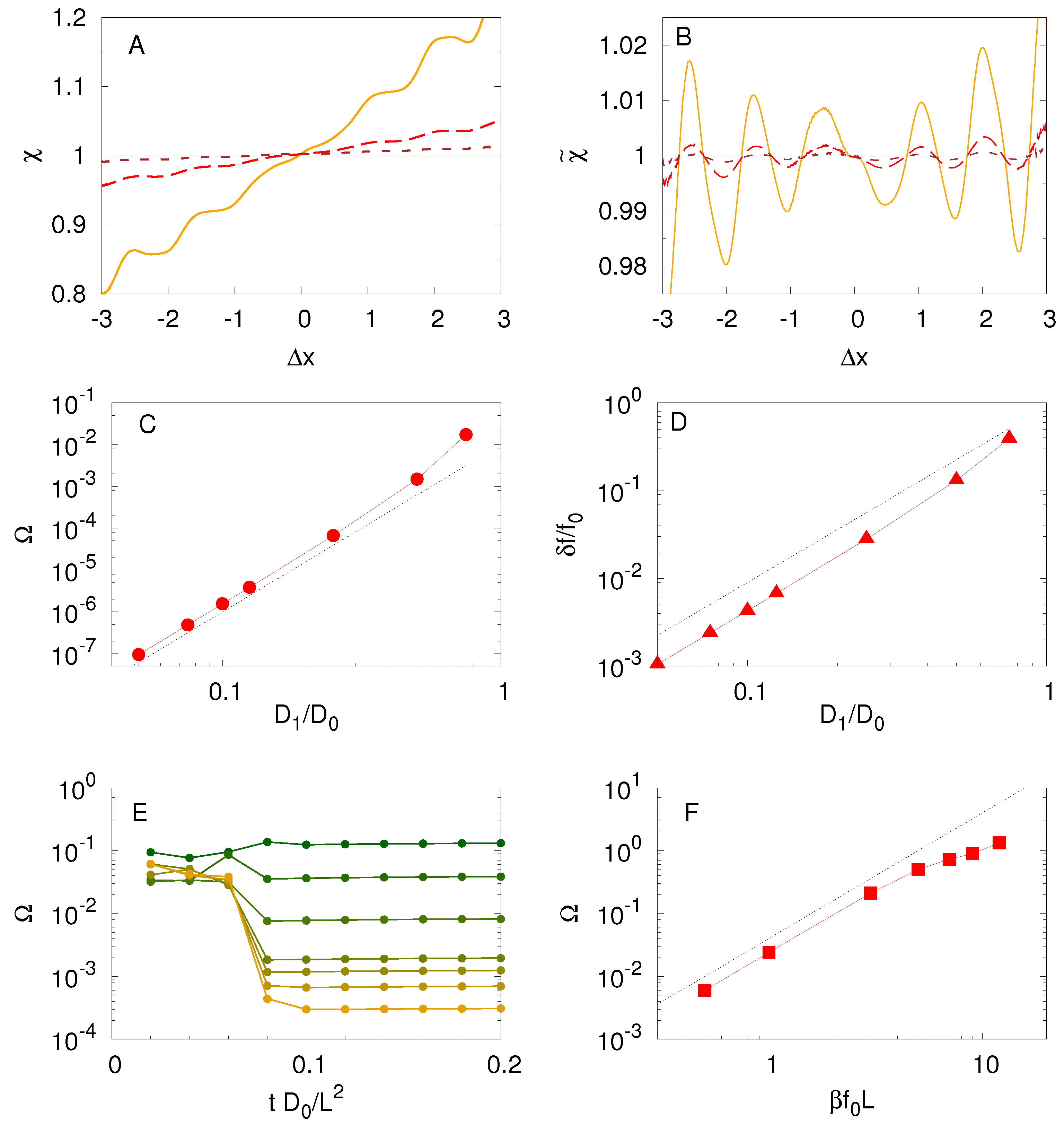
3.1. Diffusion in an Inhomogeneous Unbounded Medium

We consider the motion of a Brownian particle moving under the action of a constant force in a medium characterized by a spatially varying diffusion coefficient
D ( x ) = D 0 + D 1 sin 2 π x L
The corresponding Smoluchowski equation reads
t p ( x , t ) = x D ( x ) β p ( x , t ) f 0 D ( x ) x p ( x , t ) .
We have solved Equation (15) numerically, by means of a Lax–Wendroff method, with initial condition p ( x , 0 ) = δ ( x ) , and over a channel made by 10 identical units, each of which is periodic with period L, where we have assumed periodic boundary conditions at the channel ends, located at x = ± 5 L . To avoid the interference of periodic images, we have followed the evolution of the particle displacement probability up to a maximum time T m a x , defined as the time at which the ratio θ = p ( ± 5 L , T m a x ) / p ( 0 , T m a x ) between the probability of particles at the system edges and the corresponding probability in the middle of the channel overcomes a threshold value(i.e., θ 10 10 ). For t < T m a x , the contribution to p ( x ) from particles at x ± 5 L is negligible.
Figure 1A shows the dependence of χ on Δ x for different values of D 1 . For D 1 = 0 , Γ reduces to Equation (4), and we recover the expected relation χ = 1 . Increasing D 1 leads to a non-Gaussian density distribution [9] and χ 1 , as shown in Figure 1A. The overall departure from Gaussianity is captured better by Ω. As shown in Figure 1C, when increasing the diffusion coefficient modulation, Ω increases and behaves as Ω ( D 1 / D 0 ) 4 , in good agreement with Equation (13).
Figure 1A shows a breakdown of the left-right symmetry superimposed on a smoother modulation of χ. Indeed, we can regard the system as being driven by an effective force f e f f = f 0 + δ f , where δ f is a bias. Hence, δ f / f 0 can be regarded as a dimensionless parameter that quantifies particle rectification arising from the interplay between the net force, f 0 , and the x-dependent diffusion coefficient (for δ f / f 0 = 0 , no rectification occurs, while for δ f 0 , the sign of δ f identifies the rectification direction).
The contribution of δ f to χ is given by
χ ˜ ( Δ x , t ) = χ ( Δ x , t ) e β δ f Δ x ,
which accounts for the deviations from Gaussianity for a system under an effective force. The second moment of χ ˜
Ω ˜ ( t ) = 1 Λ Λ / 2 Λ / 2 [ χ ˜ ( Δ x , t ) χ ˜ ( t ) ] 2 d Δ x
quantifies both the overall departure from Gaussianity and also provides a route to obtain δ f . The value of δ f that better captures the breakdown of left-right symmetry in Figure 1A can be obtained by minimizing Ω ˜ . Hence, minimizing Equation (17) leads to the following expression for δ f :
β δ f ( t ) = χ ( Δ x , t ) Δ x χ ( Δ x , t ) χ ( t ) d Δ x χ ( Δ x , t ) Δ x 2 2 χ ( Δ x , t ) χ ( t ) d Δ x Δ x χ 2 .
Interestingly, Equation (18) predicts δ f = 0 for χ χ = 0 , implying Ω = 0 . Therefore, in the present regime, no rectification occurs either at equilibrium or for systems leading to a Gaussian distribution of particle displacements. For vanishing values of D 1 and f 1 , we can approximate χ ( Δ x , t ) χ ( t ) + ξ Δ x , implying Ω ξ 2 . In the limit of ξ 0 , Equation (18) reduces to
β δ f ( t ) ξ χ ( t ) Ω .
Figure 1B displays the dependence of χ ˜ on δ f , showing the absence of any net tilt. Therefore, the linear approximation for δ f given by Equation (18) properly captures the departure of χ, and consequently of Ω, with respect to their values obtained for homogeneous diffusion, D 1 = 0 . Figure 1D shows the dependence of δ f / f 0 on the modulation in the diffusion. While for larger values of D 1 a steeper dependence is observed, for smaller modulations of the diffusion, δ f / f 0 reaches an asymptotic behavior δ f / f 0 D 1 2 . Comparing the dependence of δ f and Ω on D 1 , we notice that δ f Ω , as predicted by Equation (19). The regime of validity of Equation (13) is captured in Figure 1C, where the good agreement with the numerical solution of Equation (15) highlights the wide range of reliability of Equation (13). The temporal evolution of Ω is shown in Figure 1E. At short times, Ω displays a remarkable dependence on time and reaches a plateau at longer times, for t t 0 0.1 L 2 / D 0 . Since L < Λ , Ω relaxes to its steady value faster than particle diffusion over the relevant length scale, Λ. Finally, Figure 1F shows the dependence of Ω on the external constant force, f 0 , obtaining a quadratic dependence Ω f 0 2 , and consequently a linear dependence of δ f on f 0 (data not shown).

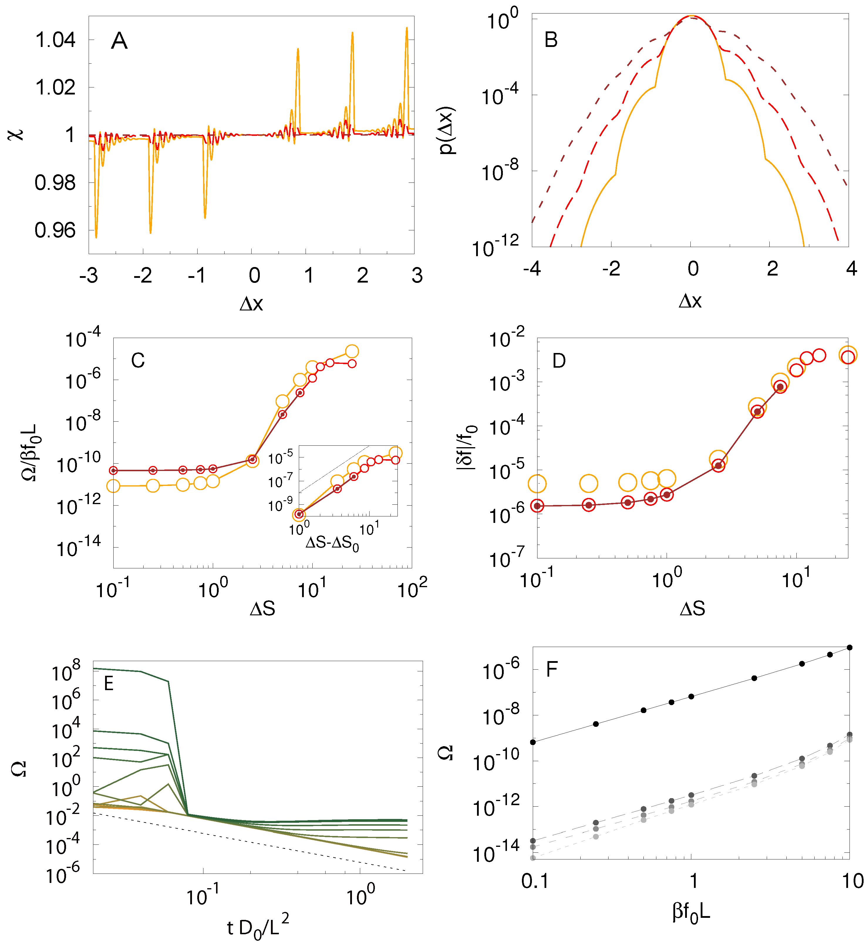
3.2. Diffusion in a Periodic Channel

We consider the diffusion of a particle in a channel of periodic half-section
h ( x ) = h 0 + h 1 cos 2 π x L ,
where L is the period, and L z the width along the z-direction, assumed to be constant. In the overdamped regime, the evolution of the probability density function, P ( x , y , z , t ) , of the particle under the action of a constant force, f 0 , is governed by the 3 D Smoluchowski equation:
t P ( x , y , z , t ) = D β · P ( x , y , z , t ) U ( x , y , z ) + D P ( x , y , z , t )
where the potential U ( x , y , z ) is given by
U ( x , y , z ) = U ( x + L , y , z ) U ( x , y , x ) = f 0 x , | y | h ( x ) & | z | L z / 2 , | y | > h ( x ) o r | z | > L z / 2
and involves both the external driving, f 0 , and the presence of boundaries. For smoothly varying channel amplitudes, x h ( x ) 1 , the diffusing particles equilibrate much faster in the transverse direction than in the main transport direction. One can then assume
( 22 ) P ( x , y , z , t ) = p ( x , t ) e β U ( x , y , z ) e β A ( x ) ( 23 ) e β A ( x ) = L z / 2 L z / 2 h ( x ) h ( x ) e β U ( x , y , z ) d y d z ,
where p ( x , t ) is the probability distribution in the coarse-grained description, and A ( x ) is the corresponding free energy
A ( x ) = f 0 x 1 β ln h x .
This quantity consists of an enthalpic contribution, f 0 x , and an entropic contribution, 1 β ln h x . This approximation shows that diffusion in 3 D can be analyzed through 1 D diffusion in the presence of entropic barriers [15,16,17,18,34]. Accordingly, we can define the dimensionless energy barrier that the particles experience along the channel,
Δ S = ln h m a x h m i n
where h m i n and h m a x are the minimum and maximum channel apertures, respectively. Integrating Equation (21) along the channel transverse section, we obtain the Fick–Jacobs equation
t p ( x , t ) = x D ( x ) β p ( x , t ) x A ( x ) + x p ( x , t ) ,
where
D ( x ) = D 0 1 + x h ( x ) 2 α
is an effective diffusion coefficient, with alpha α = 1 / 3 ( 1 / 2 ) in three (two) spatial dimensions [17]. Comparison of Equation (26) with Equation (5) shows that the geometrical confinement enters through the potential A ( x ) . Its spatial derivative gives rise to an effective force; therefore, we can understand the impact of the channel corrugation as providing a spatially-varying force acting on the Brownian particle.
We have numerically solved Equation (26) with the same numerical scheme used in the previous section. Figure 2A shows the behavior of χ. Analogously to the results reported in the previous section, χ is strongly affected by the local drift and diffusion coefficient modulation. Larger values of Δ S (i.e., larger modulations), lead to a more involved dependence of χ on Δ x , and consequently to a larger departure from the Gaussian solution obtained for Δ S = 0 . Moreover, comparing Figure 2A and Figure 1A, we notice that the qualitative and quantitative behaviors of χ differ for bounded and unbounded diffusion. While the latter case is characterized by a smoothly modulated overall extra-tilt for χ, in the former, larger modulations are overimposed to a smoothly-varying tilt, even for entropy barriers as large as Δ S = 10 .
The dependence of Ω on Δ S is also modified with respect to the behavior observed for a constant channel section, as can be appreciated comparing Figure 1C with Figure 2C. In the system analyzed, Ω shows a weaker dependence on Δ S . Disentangling the underlying mechanisms responsible for this lack of sensitivity is not straightforward, because modulations of D 1 and f 1 due to variations of the channel section compete with each other, as becomes clear in Equation (13). Nonetheless, for Δ S > 1 , using Equation (27), we have
D 1 2 e Δ S 1 e Δ S + 1
implying that D 1 2 vary very smoothly for larger Δ S . Thus, the dependence of Ω on Δ S essentially enters through the entropic force. One can assume that D 1 2 is practically constant to obtain:
Ω ( Δ S Δ S 0 ) 4
where Δ S 0 accounts for the contribution coming from the modulation in the diffusion coefficient. The inset of Figure 2C shows the good agreement of the theoretical prediction with the numerical results, up to Δ S 10 . The deviation from the behavior Ω ( Δ S Δ S 0 ) 4 observed for smaller values of Δ S is due to the time-dependence of Ω. As shown in Figure 2E, Ω reaches a quasi-steady state after a transient that depends on Δ S . For increasing entropy barriers, Δ S , the effective forces acting on a Brownian particle increase, leading to a reduction of the relaxation time, as it happens for particles in a potential well [9]. Smaller values of Δ S require longer relaxation times that cannot be considered in our numerical solution.
Even though the dependence of χ on Δ x is quite involved and does not show a clear breaking of the left–right symmetry, we have used Equation (18) to compute the rectification parameter δ f . It results that δ f ( Δ S Δ S 0 ) 4 , as shown in Figure 2D. Since Ω ( Δ S Δ S 0 ) 4 , we predict δ f Ω , which differs from the behavior observed in the previous case, in which variations of χ led to δ f Ω .
We can then conclude that different local transport mechanisms lead to different relationships between the rectification parameter and the deviations from Gaussianity inherent to Omega. Figure 2F displays the dependence of Ω on the external force, and shows that for decreasing forces, the deviation in Ω becomes vanishing small, recovering the equilibrium value Ω = 0 for β f 0 L = 0 . Moreover, Ω f 0 2 (Figure 2F), as also observed for a constant section channel (Figure 1F).

4. Discussion

We have shown that the diffusion of particles is strongly affected by heterogeneities resulting from irregularities of the boundaries or from the intrinsic nature of the host medium. The presence of local forces or of a local diffusion coefficient breaks down the Gaussian form of the probability distribution for the particles and leads to an effective rectification.
For small modulations of the spatial heterogeneities, it is possible to analyze the consequences of a non-Gaussian probability distribution. We have found that the ratio between the probabilities of forward and backward moves depends on the heterogeneities of the medium, and also on time. We have derived an expression for their ratio, Γ (Equation (6)), that is valid for small modulations both in the forcing and/or in the diffusion coefficient. In order to quantify the average deviation from Gaussian behavior, higher moments of Γ are insightful. The functional shape of the second moment Ω of Γ shows that the corrections to Γ induced by local transport are proportional to the dispersion of the modulation. When both force and diffusion coefficient are modulated, Equation (13) predicts that different regimes can be achieved, depending on the constructive or destructive interaction between the two mechanisms.
To test our predictions, we have checked Equation (13) for two different scenarios, namely a particle moving in an inhomogeneous medium with a position-dependent diffusion coefficient, and a particle in a channel of varying cross-section in the presence of entropic forces. In the first case, the force exerted is constant, whereas the diffusion coefficient depends on position. In the latter case, both the geometrically-induced effective force and the local particle diffusion coefficient depend on particle’s position along the channel. In both situations, we observe a remarkable agreement between the numerical results and our prediction for Ω in the case of mild variations in the forcing and/or medium heterogeneities.
The coupling between local forcing and diffusion can also lead to particle rectification; our analysis predicts when rectification emerges and identifies an effective parameter, δ f , which quantifies the effective rectification. In particular, our analysis reveals how the dependence of rectification on the departure from Gaussianity is affected by the physical mechanism responsible for local transport. These results suggest a possible way to characterize the intrinsic properties of the host medium and of the confinement based on the use of the new fluctuation relation and the tracking of the particles.
multiple

Acknowledgments

We acknowledge MINECO and DURSI for financial support under projects FIS 2015-67837-P and 2014SGR-922, respectively. J. Miguel Rubi and Ignacio Pagonabarraga acknowledges financial support from Generalitat de Catalunya under program Icrea Academia. Paolo Malgaretti thanks Marco Ribezzi for useful discussions.

Author Contributions

Paolo Malgaretti, Ignacio Pagonabarraga and J. Miguel Rubi conceived and designed the work; Paolo Malgaretti performed the numerical simulations and analytical calculations; Paolo Malgaretti, Ignacio Pagonabarraga and J. Miguel Rubi analyzed the results; Paolo Malgaretti, Ignacio Pagonabarraga and J. Miguel Rubi wrote the paper. All the authors have read and approved the final manuscript.

Conflicts of Interest

The authors declare no conflict of interest.

Appendix A

Here we derive the expression for Ω given by Equation (13). Substituting Equation (10) into Equation (12) and remembering that χ = 1 when calculated by Equation (11), we obtain:
Ω = ρ 1 ( Δ x , t ) ρ 0 ( Δ x , t ) ρ 1 ( Δ x , t ) ρ 0 ( Δ x , t ) 2 d Δ x
Remembering that ρ 0 ( Δ x , t ) = ρ 0 ( Δ x , t ) e β f 0 Δ x and assuming ρ 1 ( Δ x , t ) = ρ 1 ( Δ x , t ) e β Δ G , we obtain:
Ω = ρ 1 ( Δ x , t ) ρ 0 ( Δ x , t ) 2 e β f 0 Δ x β Δ G 1 d Δ x .
Expanding for | β f 0 Δ x Δ G | 1 , we get:
Ω = β f 0 Δ x β Δ G 2 ρ 1 ( Δ x , t ) ρ 0 ( Δ x , t ) 2 d Δ x
where we have used the fact that β f 0 Δ x β Δ G ρ 1 ( Δ x , t ) ρ 0 ( Δ x , t ) 2 d Δ x = 0 , due to the even character of ρ 1 ( Δ x , t ) ρ 0 ( Δ x , t ) 2 in the limit | β f 0 Δ x Δ G | 1 and to the odd character of β f 0 Δ x β Δ G . Finally, we expand both β Δ G and ρ 1 as a power series of the local modulation of the forcing, f 1 ( x ) , and/or diffusion coefficient, D 1 ( x ) . Since both f 1 ( x ) and D 1 ( x ) are periodic with zero mean, see Equations (14) and (24), the first non-vanishing contribution to β Δ G and ρ 1 is provided their second moment:
f 1 2 = f 1 2 ( x ) d x
D 1 2 = D 1 2 ( x ) d x
When the modulations are vanishing small, we have that ρ 1 0 and, remembering ρ 1 ( Δ x , t ) = ρ 1 ( Δ x , t ) e β Δ G , we have Δ G f 0 Δ x . Using the last expressions, we can expand Δ G and ρ 1 up to first order:
β Δ G = β f 0 Δ x + α 1 ( Δ x ) f 1 2 + α 2 ( Δ x ) D 1 2
ρ 1 ( Δ x , t ) = γ 1 ( Δ x , t ) f 1 2 + γ 2 ( Δ x , t ) D 1 2
where α 1 ( Δ x ) , α 2 ( Δ x ) , γ 1 ( Δ x , t ) , and γ 2 ( Δ x , t ) are to be determined numerically or by a path integral solution of Equation (26). Substituting Equations (A6) and () into Equation (A3), we get:
Ω = α 1 ( Δ x , t ) f 1 2 + α 2 ( Δ x , t ) D 1 2 2 · γ 1 ( Δ x , t ) f 1 2 + γ 2 ( Δ x , t ) D 1 2 2 d Δ x ρ 0 2 ( Δ x , t )
and finally, we can define the coefficient that appears in Equation (13) as:
A ( t ) = α 1 2 ( Δ x ) γ 1 2 ( Δ x , t ) d Δ x ρ 0 2 ( Δ x , t ) B ( t ) = α 2 2 ( Δ x ) γ 2 2 ( Δ x , t ) d Δ x ρ 0 2 ( Δ x , t ) C ( t ) = α 1 2 ( Δ x ) γ 2 2 ( Δ x , t ) + α 2 2 ( Δ x ) γ 1 2 ( Δ x , t ) + 4 α 1 ( Δ x ) α 2 ( Δ x ) γ 1 ( Δ x , t ) γ 2 ( Δ x , t ) d Δ x ρ 0 2 ( Δ x , t ) E ( t ) = 2 α 1 ( Δ x ) γ 2 ( Δ x , t ) + α 2 ( Δ x ) γ 1 ( Δ x , t ) α 1 ( Δ x ) γ 2 ( Δ x , t ) d Δ x ρ 0 2 ( Δ x , t ) F ( t ) = 2 α 1 ( Δ x ) γ 2 ( Δ x , t ) + α 2 ( Δ x ) γ 1 ( Δ x , t ) α 2 ( Δ x ) γ 1 ( Δ x , t ) d Δ x ρ 0 2 ( Δ x , t )

References

  1. Campisi, M.; Hänggi, P.; Talkner, P. Colloquium: Quantum fluctuation relations: Foundations and applications. Rev. Mod. Phys. 2011, 83, 771. [Google Scholar] [CrossRef]
  2. Astumian, R.D. The unreasonable effectiveness of equilibrium theory for interpreting nonequilibrium experiments. Am. J. Phys. 2006, 74, 683. [Google Scholar] [CrossRef]
  3. Astumian, R.D. Equilibrium theory for a particle pulled by a moving optical trap. J. Chem. Phys. 2007, 126, 111102. [Google Scholar] [CrossRef] [PubMed]
  4. Reguera, D.; Rubi, J.M. Thermodynamics and stochastic dynamics of transport in confined media. Chem. Phys. 2010, 375, 518–522. [Google Scholar]
  5. Ciliberto, S.; Joubaud, S.; Petrosyan, A. Fluctuations in out-of-equilibrium systems: From theory to experiment. J. Stat. Mech. 2010, 2010, P12003. [Google Scholar] [CrossRef]
  6. Gallavotti, G.; Cohen, E.G.D. Dynamical Ensembles in Nonequilibrium Statistical Mechanics. Phys. Rev. Lett. 1995, 74, 2694. [Google Scholar] [CrossRef] [PubMed]
  7. Crooks, G.E. Entropy production fluctuation theorem and the nonequilibrium work relation for free energy differences. Phys. Rev. E 1999, 60, 2721. [Google Scholar] [CrossRef]
  8. Vainstein, M.H.; Rubi, J.M. Gaussian noise and time-reversal symmetry in nonequilibrium Langevin models. Phys. Rev. E 2007, 75, 031106. [Google Scholar] [CrossRef] [PubMed]
  9. Risken, H. The Fokker-Planck Equation; Springer: Berlin/Heidelberg, Germany, 1988. [Google Scholar]
  10. Pagonabarraga, I.; Rubi, J.M. Long-range correlations in diffusive systems away from equilibrium. Phys. Rev. E 1994, 49, 267. [Google Scholar] [CrossRef]
  11. Höfling, F.; Franosch, T. Anomalous transport in the crowded world of biological cells. Rep. Prog. Phys. 2013, 76, 046602. [Google Scholar] [CrossRef] [PubMed]
  12. Maes, C.; Steffenoni, S. Friction and noise for a probe in a nonequilibrium fluid. Phys. Rev. E 2015, 91, 022128. [Google Scholar] [CrossRef] [PubMed]
  13. Bénichou, O.; Illien, P.; Oshanin, G.; Sarracino, A.; Voituriez, R. Diffusion and Subdiffusion of Interacting Particles on Comblike Structures. Phys. Rev. Lett. 2015, 115, 220601. [Google Scholar] [CrossRef] [PubMed]
  14. Marconi, U.M.B.; Malgaretti, P.; Pagonabarraga, I. Tracer diffusion of hard-sphere binary mixtures under nano-confinement. J. Chem. Phys. 2015, 143, 184501. [Google Scholar] [CrossRef] [PubMed] [Green Version]
  15. Jacobs, M.H. Diffusion Processes; Springer: Berlin/Heidelberg, Germany, 1967. [Google Scholar]
  16. Zwanzig, R. Diffusion past an entropy barrier. J. Phys. Chem. 1992, 96, 3926–3930. [Google Scholar] [CrossRef]
  17. Reguera, D.; Rubi, J.M. Kinetic equations for diffusion in the presence of entropic barriers. Phys. Rev. E 2001, 64, 061106. [Google Scholar] [CrossRef] [PubMed]
  18. Kalinay, P.; Percus, J.K. Approximations of the generalized Fick-Jacobs equation. Phys. Rev. E 2008, 78, 021103. [Google Scholar] [CrossRef] [PubMed]
  19. Kalinay, P.; Percus, J.K. Mapping of diffusion in a channel with abrupt change of diameter. Phys. Rev. E 2010, 82, 031143. [Google Scholar] [CrossRef] [PubMed]
  20. Dagdug, L.; Berezhkovskii, A.M.; Makhnovskii, Y.A.; Zitsereman, V.Y.; Bezrukov, S. Communication: Turnover behavior of effective mobility in a tube with periodic entropy pot. J. Chem. Phys. 2011, 134, 101102. [Google Scholar] [CrossRef] [PubMed]
  21. Malgaretti, P.; Pagonabarraga, I.; Rubi, J.M. Entropic transport in confined media: A challenge for computational studies in biological and soft-matter systems. Front. Phys. 2013, 1, 21. [Google Scholar] [CrossRef] [Green Version]
  22. Chacón-Acosta, G.; Pineda, I.; Dagdug, L. Diffusion in narrow channels on curved manifolds. J. Chem. Phys. 2013, 139, 214115. [Google Scholar] [CrossRef] [PubMed]
  23. Kalinay, P. Moment expansion for mapping of the confined diffusion. Phys. Rev. E 2013, 87, 032143. [Google Scholar] [CrossRef]
  24. Kalinay, P. Integral formula for the effective diffusion coefficient in two-dimensional channels. Phys. Rev. E 2016, 94, 012102. [Google Scholar] [CrossRef] [PubMed]
  25. Chinappi, M.; De Angelis, E.; Melchionna, S.; Casciola, C.M.; Succi, S.; Piva, R. Molecular Dynamics Simulation of Ratchet Motion in an Asymmetric Nanochannel. Phys. Rev. Lett. 2006, 97, 144509. [Google Scholar] [CrossRef] [PubMed]
  26. Marconi, U.M.B.; Melchionna, S.; Pagonabarraga, I. Effective electrodiffusion equation for non-uniform nanochannels. J. Chem. Phys. 2013, 138, 244107. [Google Scholar] [CrossRef] [PubMed] [Green Version]
  27. Malgaretti, P.; Pagonabarraga, I.; Rubi, J.M. Entropic Electrokinetics: Recirculation, Particle Separation, and Negative Mobility. Phys. Rev. Lett. 2014, 113, 128301. [Google Scholar] [CrossRef] [PubMed]
  28. Malgaretti, P.; Pagonabarraga, I.; Rubi, J.M. Geometrically Tuned Channel Permeability. Macromol. Symp. 2015, 357, 178–188. [Google Scholar] [CrossRef]
  29. Malgaretti, P.; Pagonabarraga, I.; Rubi, J.M. Entropically induced asymmetric passage times of charged tracers across corrugated channels. J. Chem. Phys. 2016, 144, 034901. [Google Scholar] [CrossRef] [PubMed] [Green Version]
  30. Bianco, V.; Malgaretti, P. Non-monotonous polymer translocation time across corrugated channels: Comparison between Fick-Jacobs approximation and numerical simulations. J. Chem. Phys. 2016, 145, 114904. [Google Scholar] [CrossRef]
  31. Malgaretti, P.; Pagonabarraga, I.; Rubi, J.M. Cooperative rectification in confined Brownian ratchets. Phys. Rev. E 2012, 85, 010105. [Google Scholar] [CrossRef] [PubMed]
  32. Malgaretti, P.; Pagonabarraga, I.; Rubi, J.M. Confined Brownian ratchets. J. Chem. Phys. 2013, 138, 194906. [Google Scholar] [CrossRef] [PubMed] [Green Version]
  33. Malgaretti, P.; Pagonabarraga, I.; Rubi, J.M. Working under confinement. Eur. Phys. J. Spec. Top. 2014, 223, 3295–3309. [Google Scholar] [CrossRef]
  34. Martens, S.; Schmid, G.; Schimansky-Geier, L.; Hänggi, P. Entropic particle transport: Higher-order corrections to the Fick-Jacobs diffusion equation. Phys. Rev. E 2011, 83, 051135. [Google Scholar] [CrossRef] [PubMed]
Figure 1. Fluctuation relation for a particle in a constant-amplitude channel and inhomogeneous medium, D 1 0 under a constant force β f 0 L = 0.5 . (A) χ as function of the displacement, Δ x , at t D 0 / L 2 = 0.2 for different values of the diffusion coefficient modulation: D 1 D 0 = 0.125 , 0.25 , 0.5 for dotted (brown), dashed (red), and solid (orange) lines, respectively. (B) χ ˜ as a function of Δ x for the same parameters as in panel A, where δ f has been calculated using Equation (18). (C) Ω as a function of D 1 / D 0 for β f 0 L = 0.5 with Λ = 4 and t D 0 / L 2 = 0.2 ; dotted line stands for Ω ( D 1 / D 0 ) 4 . (D) δ f / f 0 as function of D 1 / D 0 for the same parameters as in panel C; dotted line stands for δ f / f 0 ( D 1 / D 0 ) 2 . (E) Ω as a function of time normalized by τ = L 2 / D 0 with Λ = 4 , for D 1 / D 0 = 0.05 , 0.075 , 0.1 , 0.25 , 0.5 , 0.75 ; the darker the line, the larger the ratio D 1 / D 0 . (F) Ω as a function of the driving force β f 0 L for D 1 / D 0 = 0.5 .
Entropy 18 00394 g001
Figure 2. Fluctuation relation for a Brownian particle in a varying-amplitude channel, h 1 0 , that induces a modulation in the effective diffusion coefficient, D 1 0 , for a constant force β f 0 L . (A) χ as function of the displacement, Δ x , for t D 0 / L 2 = 2 , with β f 0 L = 1 and different values of the entropic barrier Δ S = 0.1 , 1 , 10 for dotted (brown), dashed (red), and solid (orange) line, respectively. (B) p ( Δ x ) as function of Δ x for the same values of the parameters as in panel A. (C) Ω at t D 0 / L 2 = 2 , as a function of Δ S for β f 0 L = 0.1 , 1 , 10 bigger points standing for larger Δ S , with Λ = 4 . Inset: Ω as a function of the reduced entropic barrier Δ S Δ S 0 , with Δ S 0 = 1.5 , for the same value of the parameters in the main figure; dotted line stands for Ω ( Δ S Δ S 0 ) 4 . (D) | δ f | / f 0 as function of Δ S for the same value of the parameters in panel C. (E) Ω as a function of time normalized by τ = L 2 / D 0 for Δ S = 0.1 , 0.25 , 0.5 , 0.75 , 1 , 2.5 , 5 , 7.5 , 10 , darker lines standing for larger values of Δ S . (F) Ω as a function of the forcing β f 0 L for Δ S = 0.1 , 0.5 , 1 , 5 darker lines standing for higher values of Δ S , being Λ = 4 .
Entropy 18 00394 g002

