The Optimal Confidence Intervals for Agricultural Products’ Price Forecasts Based on Hierarchical Historical Errors

Abstract

With the levels of confidence and system complexity, interval forecasts and entropy analysis can deliver more information than point forecasts. In this paper, we take receivers’ demands as our starting point, use the trade-off model between accuracy and informativeness as the criterion to construct the optimal confidence interval, derive the theoretical formula of the optimal confidence interval and propose a practical and efficient algorithm based on entropy theory and complexity theory. In order to improve the estimation precision of the error distribution, the point prediction errors are STRATIFIED according to prices and the complexity of the system; the corresponding prediction error samples are obtained by the prices stratification; and the error distributions are estimated by the kernel function method and the stability of the system. In a stable and orderly environment for price forecasting, we obtain point prediction error samples by the weighted local region and RBF (Radial basis function) neural network methods, forecast the intervals of the soybean meal and non-GMO (Genetically Modified Organism) soybean continuous futures closing prices and implement unconditional coverage, independence and conditional coverage tests for the simulation results. The empirical results are compared from various interval evaluation indicators, different levels of noise, several target confidence levels and different point prediction methods. The analysis shows that the optimal interval construction method is better than the equal probability method and the shortest interval method and has good anti-noise ability with the reduction of system entropy; the hierarchical estimation error method can obtain higher accuracy and better interval estimation than the non-hierarchical method in a stable system.

1. Introduction

According to price forecasts, producers and managers adjust current productions and operations, and governments make proper macro-economic policy to stabilize prices. A great number of studies shows that price forecasts of agricultural products are meaningful [1,2]. Nowadays, the price forecasts of agricultural products are mainly based on the point forecasts. However, interval forecasts can deliver more information than point forecasts. Point forecasting is widely used, can provide a single value of the variable in the future and cannot provide any information about the value of uncertainty. Uncertainty information is particularly important for decision makers with different risk preferences. The result of interval forecasts is an interval with a confidence level, which is more convenient for decision makers to formulate risk management strategies. Due to the importance of interval forecasts, in the monthly World Agricultural Supply and Demand Estimates (WASDE) of the United States Department of Agriculture (USDA), price forecasts are published in the form of intervals.

The more stable and simple the price system of agricultural products, the more favorable the price forecast. Entropy is a measure of the complexity of a system. Greater entropy means that the system is more complex, and then, the price forecast is prone to distortion. Su et al. [3] verified that there is chaos in the price system by calculating the Kolmogorov entropy. Their price system has positive entropy; but the entropy is not big, and the system has weak chaos. How do we predict prices in such a system? When entropy is not big, can we obtain better forecasting results? In this paper, we illustrate that this price system can be forecasted, and we verify that the price interval forecast is feasible in the system with positive Kolmogorov entropy. Our paper illustrates that we can obtain the interval forecasts. In recent years, many scholars have carried out research work on entropy in the economic field. Bekiros et al. [4] studied the dynamic causality between stock and commodity futures markets in the United States by using complex network theory. We utilize the extended matrix and the time varying network topology to reveal the correlation and the temporal dimension of the entropy relationship. Selvakumar [5] proposed an enhanced cross-entropy (ECE) method to solve the dynamic economic dispatch (DED) problem with valve-point effects. Fan et al. [6] used multi-scale entropy analysis; we investigate the complexity of the carbon market and the average return trend of daily price returns. Billio et al. [7] analyzed the temporal evolution of systemic risk in Europe by using different entropy measures and constructed a new banking crisis early warning indicator. Ma and Si [8] studied a continuous duopoly game model with a two-stage delay. They investigated the influence of delay parameters on the stability of the system.

In agricultural economics, Teigen and Bell [9] established the confidence interval of the corn price by the approximate variance of the forecast. Prescott and Stengos [10] applied the bootstrap method to construct the confidence interval of the dynamic metering model and forecasted the pork supply. Bessler and Kling [11] affirmed the role of probability prediction and defined what is a “good” prediction. Sanders and Manfredo [12], Isengildina-Massa et al. [13] compared four methods, including the histogram method, the kernel density method, the parameter distribution estimation method and the quantile regression method. They evaluated the confidence intervals generated by these methods. The results showed that the kernel function method and the quantile regression method can get the best interval forecasts.

There are two main methods for interval forecasting. One is the prediction of the interval type data [14]. The interval type data are composed of the minimum and maximum sequences. This method can be used in a case with comprehensive information. The disadvantage is that it cannot provide the confidence level of the interval. The other is constructing the confidence interval by the estimation of the errors of point forecasts. The advantage is that one can obtain confidence levels. In this paper, we will construct a forecast interval with some target confidence level based on the entropy theory and system complexity theory.

In practice, the prediction interval of the same target confidence is not unique, so which is the best interval? Decision makers often choose those results that meet their own needs, so we can directly build the “optimal” forecast intervals under their standard. In this paper, we will construct the model of the optimal forecast interval and transform this problem to an optimization problem. Since it is difficult to solve the analytic solution for a nonlinear optimization problem, we establish an algorithm to solve the numerical solution.

Nowadays, the optimal criterion of the interval mainly lies in the accumulation of the accuracies of point forecasts. The M index defined by Batu [15] is an average of point forecast errors in the prediction interval. Demetresc [16] used the cumulative accuracy of the point forecasts, which can obtain longer intervals and high reliability. However, for the economic data, this kind of forecast loses significance. The forecast interval not only delivers accuracy, but also delivers information. How does one evaluate the interval from both the accuracy and the informativeness, which seem to be contradictory aspects? Yaniv and Foster [17] provided a formal model of the binary loss function, i.e., the trade-off model between accuracy and informativeness. They compared their model with many common models. The results showed that their model is more suitable to reflect individual preferences. In this paper, the optimal forecast interval model is established by using the trade-off model.

To obtain the confidence level, it is critical to correctly estimate the error distribution of the point forecasts. In general, the error distribution is supposed to be a normal distribution or a ${\mathsf{\chi }}^2$ distribution, etc. However, this method is subjective, and it is possible that the error distribution does not obey the assumed distribution. Gardner [18] found that prediction intervals generated by the Chebyshev inequality are more accurate than those generated by the hypothesis of the normal distribution, which was opposed by Bowerman and Koehler [19], Makridakis and Winkler [20] and Allen and Morzuch [21]. They thought the intervals generated by the Chebyshev inequality are too wide. Stoto [22] and Cohen [23] found that the forecast errors of population growth asymptotically obey the normal distribution. Shlyakhter et al. [24], recommended the exponential distribution in the data of population and energy. Willia and Goodman [25] first used the empirical method to estimate the distribution of historical errors of point forecasts without restrictions on the method of the point forecast. Chatfield [26] pointed out that the empirical method is a good choice when the error distribution is uncertain. Taylor and Bunn [27] first applied the quantile regression for the interval estimation. Hanse [28] used semi-parametric estimation and the quantile method to construct the asymptotic forecast intervals. This method has strict requirements on time series. Demetrescu [16] pointed out that quantile regressions are not so useful, since one does not know in advance which quantile is needed, and an iterative procedure would have obvious complexity. Jorgensen and Sjoberg [29] used the nonparametric histogram method to find the points of the software development workload distribution. Yan et al. [30], thought that the errors of point forecasts have great influence on the accuracy of uncertainty analysis. Ma et al. [31] investigated existence and the local stable region of the Nash equilibrium point. Ma and Xie [32] studied financial and economic system under the condition of three parameters’ change circumstances, Zhang and Ma [33] and ou and Ma [34] investigated a class of the nonlinear system modeling problem, with good research results. Martínez-Ballesteros et al. [35] forecasted by means of association rules. Ren and Ma deepen and complete a kind of macroeconomics IS-LM model with fractional-order calculus theory, which is a good reflection on the memory characteristics of economic variables.

The novelty of this paper is in providing two methods. One is the stratified historical errors’ estimation, and the other is the optimal confidence interval model.

To improve the estimation accuracy, we try to stratify the historical error data according to the price and estimate the error distribution of each layer. In the estimation of the historical error distribution, all errors are often treated as obeying the same distribution. Considering the heteroscedasticity of prediction errors of different prices, it is too rough. The frequencies of different prices in history are different. Some extreme prices in history only appeared several times with the emergence of sharp fluctuations. The forecast errors of these prices are generally large, and the sample capacity of such errors is small. On the contrary, some prices appear very frequently with small fluctuations. The forecast errors of these prices are generally small, and the sample capacity of such errors is big. Therefore, we stratify the historical error data according to different prices and estimate the error distribution of each layer.

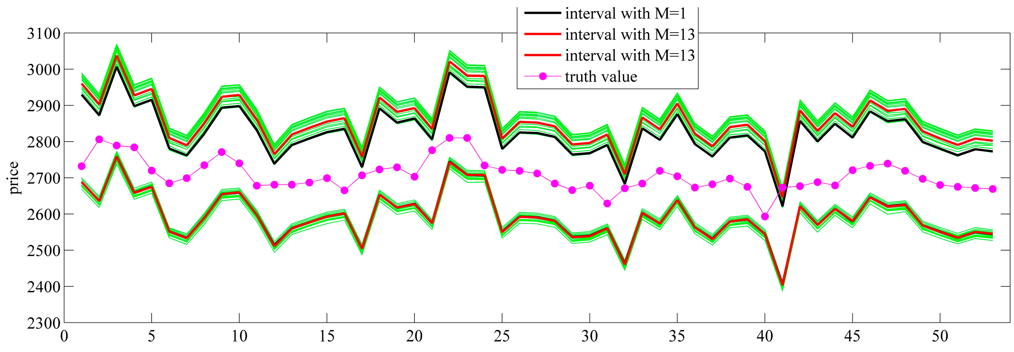
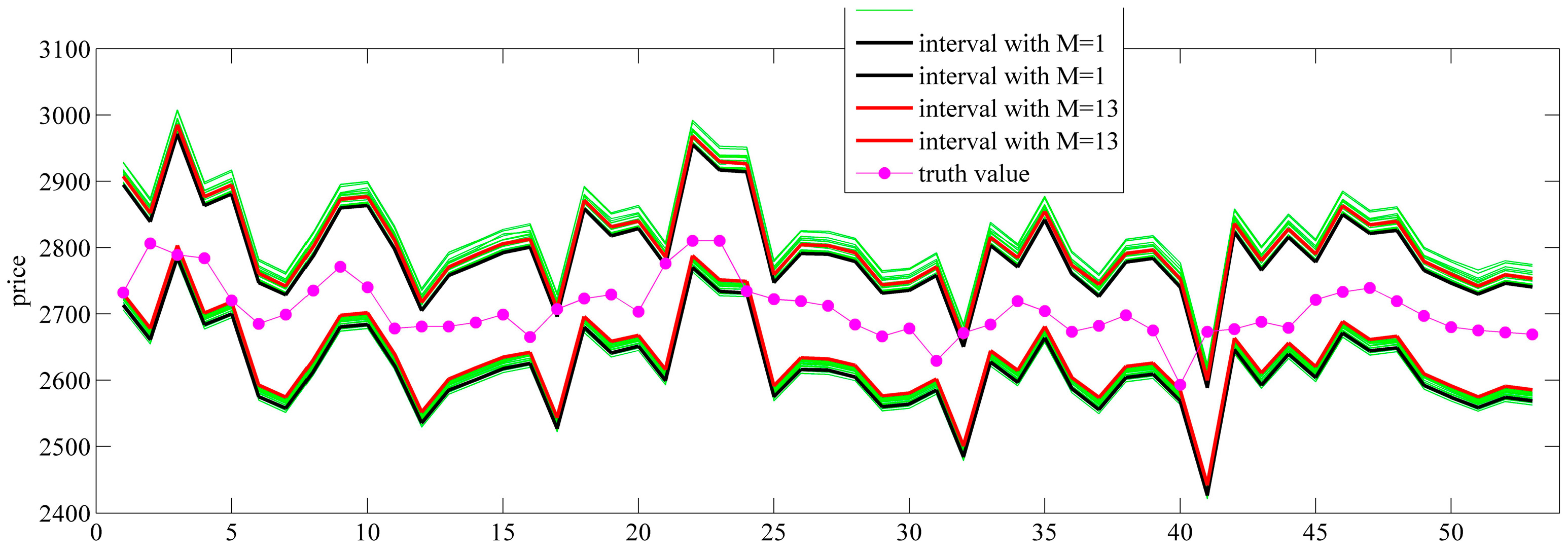
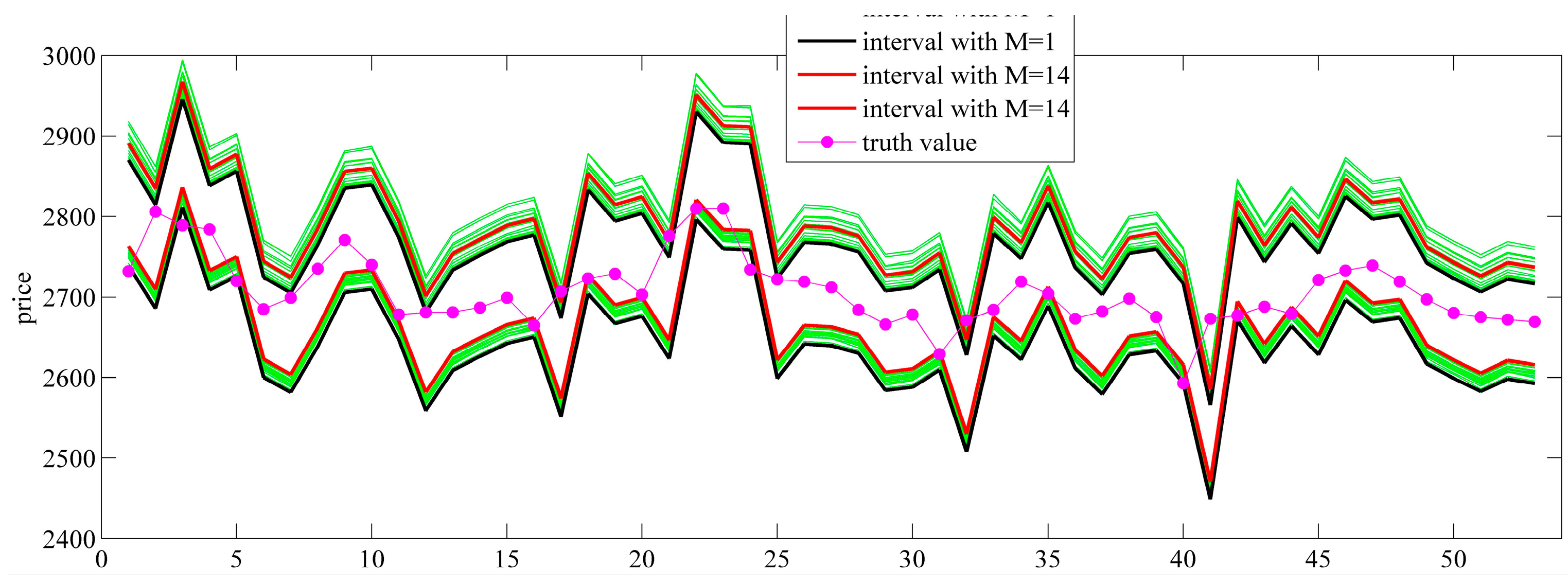
In this paper, we induce the model of the optimal confidence interval according to the accuracy and the informativeness trade-off model, provide a practical and efficient algorithm for the optimal confidence interval model based on the complexity of the forecasting system and estimate the error distributions according to the stratified prices. The kernel function method is used to estimate the error distribution. For different target confidence levels, simulation prediction is achieved for the continuous futures daily closing prices of soybean meal and non-GMO soybean. Unconditional coverage, independence and conditional coverage tests are used to evaluate the interval forecasts. Empirical analysis is divided into two subsections. In Section 5.1, we apply the equal probability method, the shortest interval method and the optimal interval method to construct the prediction intervals, compare their loss functions and test whether the intervals generated by the optimal interval method are optimal. We add the various SNR (Signal-Noise Ratio) noises to the historical error data and the prediction prices and test the robustness of the algorithm. In Section 5.2, the prediction errors are divided into one to 20 layers according to the prices. The error distributions are estimated in different layers. The confidence intervals are constructed and evaluated, finding whether the error stratification method can improve the prediction accuracy. The evaluation indices are concluding from the loss function, interval endpoint, interval midpoint, interval length, coverage, unconditional coverage test statistic, independence test statistic and conditional coverage test statistic. The error data, including point forecast errors generated by the weighted local method and the RBF neural network method, are used to investigate whether the hierarchical estimation error method can improve the prediction accuracy for different point forecasts.

2. The Model and Algorithm of the Optimal Confidence Intervals

Denote by $Y_t$ the process to be forecast, and assume it has a continuous and strictly increasing cumulative distribution function. Suppose $f_t=f_{Y_t|{\mathsf{\Psi }}_{t-1}}$ is the conditional density of $Y_t$ on its past ${\mathsf{\Psi }}_{t-1}=\{Y_{t-1},Y_{t-2},\dots \}$, and $F_t=F_{Y_t|{\mathsf{\Psi }}_{t-1}}$ is the conditional cumulative distribution function of $Y_t$. Clearly, the confidence interval $[L_t,U_t]$$(L_t<U_t)$ of $Y_t$ with confidence level ${\alpha }_0(0<{\alpha }_0<1)$ satisfies:

$$P(L_t\le Y_t\le U_t|{\mathsf{\Psi }}_{t-1})={\displaystyle {\int }_{L_t}^{U_t}{f}_t(y)dy}=F_t(U_t)-F_t(L_t)={\alpha }_0$$

(1)

Yaniv and Foster [17] established the accuracy-informativeness trade-off model:

$$\mathcal{L}=f\left[\left|\frac{y-m}{g}\right|,\ln (g)\right],$$

where the first variable evaluates accuracy, the second variable evaluates informativeness, $y$ is a truth value, $m$ is the midpoint of prediction interval and $g$ denotes the width of interval. Actually, the accuracy-informativeness trade-off model is a kind of loss function. Yaniv and Foster [17] thought that, for a good interval, the lower the $\mathcal{L}$ score, the better. They gave a concrete expression of $\mathcal{L}$:

$$\mathcal{L}=\left|\frac{y-m}{g}\right|+\gamma \ln (g),$$

where the coefficient $\gamma \ge 0$ is a trade-off parameter that reflects the weights placed on the accuracy and informativeness of the estimates. Yaniv and Foster [17] supposed that the value of $\gamma$ is taken from 0.6 to 1.2, close to one.

For a given confidence level${}_{{\alpha }_0}$, we take the minimum $\mathcal{L}$ as the objective to solve the optimal confidence interval, which can be transformed to find the solution $\left(\begin{array}{l}{L}_t\ast \\ U_t\ast \end{array}\right)$ of the nonlinear optimization problem under the condition ${\mathsf{\Psi }}_{t-1}$, where:

$$\left(\begin{array}{l}{L}_t\ast \\ U_t\ast \end{array}\right):=\underset{L_t,U_t\in {\mathcal{D}}_t}{\arg \hspace{0.17em}\min } E({\mathcal{L}}_t|L_t\le Y_t\le U_t).$$

Denote by ${\mathcal{D}}_t$ the set of all possible values of $Y_t$; the constraint conditions are:

$$\begin{array}{l}(\mathrm{i})\hspace{0.17em}{F}_t(U_t\ast )-F_t(L_t\ast )={\displaystyle {\int }_{L_t\ast }^{U_t\ast }{f}_t(y)dy}={\alpha }_0;\\ \left(\mathrm{ii}\right)\hspace{0.17em}{L}_t\ast <U_t\ast \end{array}$$

Then, we can obtain the following simplified objective function.

Proposition 1.

$$E({\mathcal{L}}_t|L_t\le Y_t\le U_t)={\displaystyle {\int }_{L_t}^{U_t}\left[\left|\frac{y-\frac{L_t+U_t}{2}}{U_t-L_t}\right|+\gamma \ln \left(U_t-L_t\right)\right]f_t(y)dy}$$

(2)

Proof. 

See Appendix A.

Thus, we only need to find the solution $\left(\begin{array}{l}{L}_t\\ U_t\end{array}\right)$ that can minimize $E({\mathcal{L}}_t|L_t\le Y_t\le U_t)$ of (2) and that satisfies $F_t(U_t)-F_t(L_t)={\alpha }_0$ with $L_t<U_t$. It is difficult to solve analytic solutions; however, for a strictly increasing and numerical $F_t$, we can establish an algorithm to obtain numerical solutions. The steps are as follows.

Step 1. Take all $L_t,U_t\in {\mathcal{D}}_t$ and $L_t<U_t,$ and find all $\left(\begin{array}{l}{L}_t\\ U_t\end{array}\right)$ satisfying $F_t(U_t)-F_t(L_t)={\alpha }_0$, i.e.,$\left(\begin{array}{l}{L_t}^1\\ {U_t}^1\end{array}\right),\left(\begin{array}{l}{L_t}^2\\ {U_t}^2\end{array}\right),\dots .$ Since the value $F_t(U_t)-F_t(L_t)$ increases with the increase of $U_t$ for a fixed $L_t$, the value of $U_t$ can be solved uniquely. Therefore, we point out that it is not necessary to take all of the values of ${\mathcal{D}}_t$.

Step 2. For each point obtained from the first step $\left(\begin{array}{l}{L_t}^1\\ {U_t}^1\end{array}\right),\left(\begin{array}{l}{L_t}^2\\ {U_t}^2\end{array}\right),\dots$, calculate the midpoint $M_t^i=\frac{L_t^i+U_t^i}{2}$.

Step 3. For every $\left(\begin{array}{l}{L}_t^i\\ M_t^i\\ U_t^i\end{array}\right)$, compute:

$${\mathcal{L}}_t^i=\left(\frac{1}{2}+\gamma \ln \left(U_t^i-L_t^i\right)\right){\alpha }_0+\frac{1}{U_t^i-L_t^i}\left({\displaystyle {\int }_{L_t^i}^{\frac{L_t^i+U_t^i}{2}}{F}_t(y)dy}-{\displaystyle {\int }_{\frac{L_t^i+U_t^i}{2}}^{U_t^i}{F}_t(y)dy}\right)$$

Step 4. Sort all of the ${{\mathcal{L}}_t}^1,{{\mathcal{L}}_t}^2,\dots$; find the smallest ${\mathcal{L}}_t\ast$; and record the corresponding $\left(\begin{array}{l}{L}_t\ast \\ M_t\ast \\ U_t\ast \end{array}\right)$

3. Estimate the Conditional Probability Distribution of Error

Denote by ${\widehat{Y}}_t$ the forecast of $Y_t$ and by $e_t=Y_t-{\widehat{Y}}_t$ the error, i.e.,

$$Y_t={\widehat{Y}}_t+e_t.$$

(3)

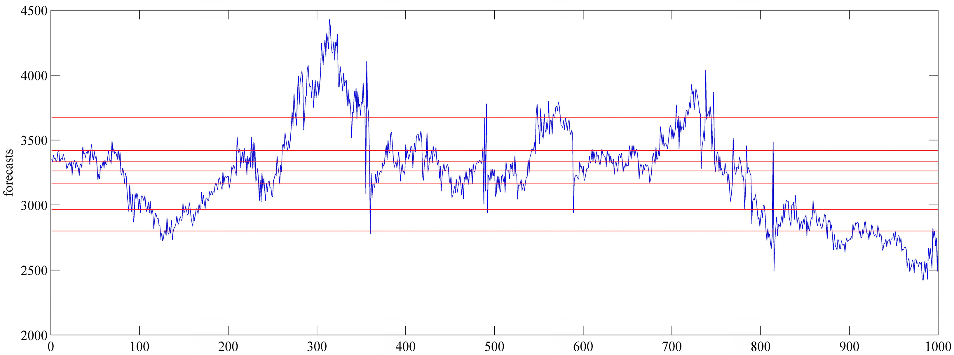
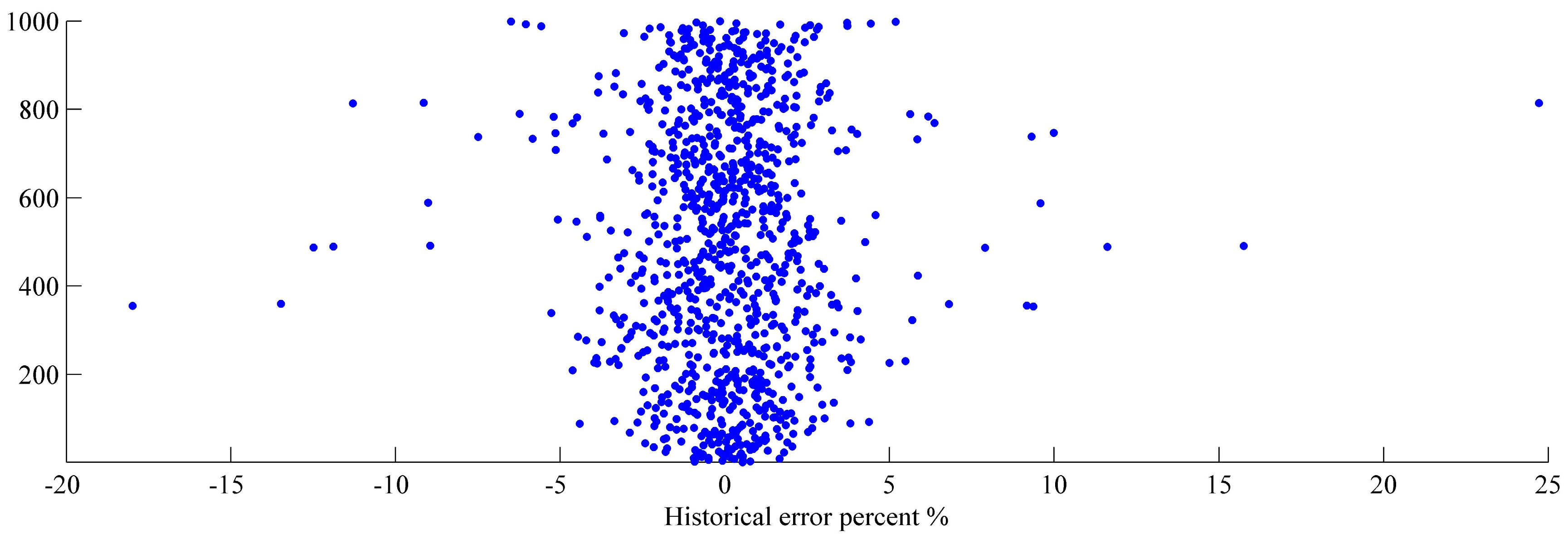
If we take ${\widehat{Y}}_t$ as the optimal point forecast [27], we can estimate $e_t$ and obtain the distribution of $Y_t$. In this paper, we apply the empirical method, which means that we can take all obtained point forecast errors as samples of the same probability distribution. We estimate the probability distribution by the kernel function method, for which we give the details below. However, it is rough to take all obtained errors as obeying one distribution. For one forecasting value, if we can collect all corresponding errors, the errors can be considered to obey one distribution. However, in general, the error sample size of one forecasting value is very small. In order to collect as many samples as possible, we can take the errors of one forecasting interval. Therefore, how to choose reasonable forecasting value intervals is very important.

We stratify the prediction error samples evenly according to the forecasting values. First, we divide the N historical forecasting values $\left\{{\widehat{Y}}_k,k=t-1,t-2,\dots ,t-N\right\}$ into $M$ layers, i.e., M intervals, and record the upper limit and lower limit of every layer. The size of every layer is about $N/M.$ The size of every layer may not be the same, and a 10% difference is admissible. Second, put the errors of every layer forecasts into the error sample set of the layer. For example, when $N=1000$, $M=8$, the division of the forecasts is shown in Figure 1.

When N is fixed, the bigger $M$ is, the smaller $N/M$ is; the smaller $M$ is, the greater $N/M$ is. When $N/M$ is small, the size of the sample is small, and the estimating accuracy declines. When $N/M$ is big, the size of the sample is big, which means the width between two adjacent red lines in Figure 1 will be bigger. At this time, the forecasting values within the same layer have a big difference; taking the errors in this layer as obeying the same probability distribution is not reasonable. In short, $M$ cannot be taken too big or too small. When N is fixed, there is an optimal $M$ to obtain the optimal estimated error distribution, which will be verified in Section 5.

For fixed N and $M$ ($N>M$), we apply the kernel function method to estimate the error distribution. Assume that the size of each layer is $N/M$; the error sequence of the $i-\mathrm{th}\hspace{0.17em}(i=1,2,\cdots ,M)$ layer is ${\text{{}\mathrm{e}}_{ik},k=1,2,\cdots ,K_M\}$. Then, the density estimation of the sequence at point $x$ is ${\widehat{f}}_i(x)=\frac{1}{K_M}{\displaystyle \sum _{k=1}^{K_M}\varphi \left(x-e_{ik};h_i\right)}$, where $\varphi$ is the normal kernel function:

$$\varphi \left(u;h\right)=\frac{1}{\sqrt{2\pi }h}\exp \{-\frac{u^2}{2h^2}\}$$

$h_i$ is the bandwidth or smoothing parameter. In this paper, we apply the optimal bandwidth [30] $h_i={\left(\frac{4}{3K_M}\right)}^{\frac{1}{5}}{\tilde{\sigma }}_i$, where ${\tilde{\sigma }}_i=\mathrm{median}\left\{\right|e_{ik}-{\tilde{\mu }}_i\left|\right\}/0.6745$, and ${\tilde{\mu }}_i$ represents the sample median.

4. Evaluation of the Prediction Interval

The accuracy of forecast intervals is traditionally examined in terms of coverage. However, only if test values are enough, the coverage can reflect the true confidence level. Bowman [36] describes the use of smoothing techniques in statistics, including both density estimation and nonparametric regression. Christoffersen [37] developed approaches to test the coverage and independence in terms of hypothesis tests. Since his methods do not make any assumption about the true distribution, they can be applied to all empirical confidence intervals. His methods include unconditional coverage, independence and conditional coverage tests.

Suppose that ${\alpha }_0$ is the confidence level, and test sample sequence is ${\text{{}\mathrm{e}}_t,t=1,\cdots ,N_2\}$. First, denote by $I_t$ the indicator:

$$I_t=\{\begin{array}{l}1,\hspace{0.17em}if\hspace{0.17em}{e}_t\in [L_{t|t-1}({\alpha }_0),U_{t|t-1}({\alpha }_0)]\\ 0,\hspace{0.17em}if\hspace{0.17em}{e}_t\notin [L_{t|t-1}({\alpha }_0),U_{t|t-1}({\alpha }_0)]\end{array}$$

where $[L_{t|t-1}({\alpha }_0),U_{t|t-1}({\alpha }_0)]$ is an out-of-sample prediction interval, which denotes the prediction interval of $e_t$ constructed by the $(t-1)-\mathrm{th}$ error; $L_{t|t-1}({\alpha }_0)$ and $U_{t|t-1}({\alpha }_0)$ are the lower limit and upper limit, respectively. Christoffersen [37] proved that ${\displaystyle \sum _{t=1}^{N_2}{I}_t}$ obeys the binomial distribution $B(N_2,{\alpha }_0)$. When the capacity of test sample is finite, Christoffersen [37] constructed a standard likelihood ratio test with the null hypothesis $H_0:E(I_t|{\Omega }_{t-1})={\alpha }_0$ and the alternative hypothesis $H_1:E(I_t|{\Omega }_{t-1})\ne {\alpha }_0$. The purpose is to examine, with condition ${\Omega }_{t-1}$, whether ${\displaystyle \sum _{t=1}^{N_2}{I}_t}$ equals ${\alpha }_0$ significantly. If $H_0$ is accepted, then the coverage of the test sample equals the target confidence level. Christoffersen [37] established the following test statistic:

$$L{R}_{uc}(\alpha )=-2\ln \frac{L(\alpha ;I_1,I_2,...I_{N_2})}{L(\widehat{p};I_1,I_2,...I_{N_2})}$$

When the null hypothesis holds, $L{R}_{uc}(\alpha )\stackrel{asy}{\sim }{\chi }^2(1)$ and ${\chi }^2(1)$ represent the chi-squared distribution which degree of freedom is 1, where $L(\alpha ;I_1,I_2,...I_{N_2})={(1-\alpha )}^{n_0}{\alpha }^{n_1}$, $\widehat{p}=\frac{n_1}{n_0+n_1}$ is the maximum likelihood estimation of ${\alpha }_0$, and $n_0$ and $n_1$ denote the number that $\left\{I_t\right\}$ “hit” zero and one, respectively.

Christoffersen [37] thought that the unconditional test is insufficient when the dynamics are present in the higher order moments. In order to test the independence, he introduced a binary first-order Markov chain with transition probability matrix:

$${\Pi }_1=\left[\begin{array}{ccc}1-{\pi }_{01}& & {\pi }_{01}\\ 1-{\pi }_{11}& & {\pi }_{11}\end{array}\right],$$

(4)

where ${\pi }_{ij}=P(I_t=j|I_{t-1}=i)$. If independence holds true, then ${\pi }_{ij}={\pi }_j,i,j=0,1$, where ${\pi }_j=P(I_t=j)$. Therefore, under the null hypothesis of independence, (4) turns to:

$${\Pi }_2=\left[\begin{array}{ccc}1-{\pi }_1& & {\pi }_1\\ 1-{\pi }_1& & {\pi }_1\end{array}\right]$$

We can estimate ${\pi }_{ij},{\pi }_j$ by the test sample frequency, i.e.,

$${\widehat{\Pi }}_1=\left[\begin{array}{ccc}\frac{n_{00}}{n_{00}+n_{01}}& & \frac{n_{01}}{n_{00}+n_{01}}\\ \frac{n_{10}}{n_{10}+n_{11}}& & \frac{n_{11}}{n_{10}+n_{11}}\end{array}\right]$$

Additionally, ${\widehat{\pi }}_1=\frac{n_{01}+n_{11}}{n_{00}+n_{10}+n_{01}+n_{11}}$. The test statistic under the null hypothesis is:

$$L{R}_{ind}=-2\ln \frac{L({\widehat{\Pi }}_2;I_1,I_2,...I_{N_2})}{L({\widehat{\Pi }}_1;I_1,I_2,...I_{N_2})}\stackrel{asy}{\sim }{\chi }^2(1)$$

where $L({\widehat{\Pi }}_1)={(1-{\widehat{\pi }}_{01})}^{n_{00}}{{\widehat{\pi }}_{01}}^{n_{01}}{(1-{\widehat{\pi }}_{11})}^{n_{10}}{{\widehat{\pi }}_{11}}^{n_{11}}$, $L({\widehat{\Pi }}_2)={(1-{\widehat{\pi }}_1)}^{n_{00}+n_{10}}{{\widehat{\pi }}_1}^{n_{01}+n_{11}}$.

The above tests for unconditional coverage and independence are now combined to form a complete test of conditional coverage:

$$L{R}_{\mathrm{cc}}=-2\ln \frac{L(\alpha ;I_1,I_2,...,I_{N_2})}{L({\widehat{\Pi }}_1;I_1,I_2,...,I_{N_2})}\stackrel{asy}{\sim }{\chi }^2(2).$$

5. Empirical Analysis

In this paper, the continuous futures daily closing prices of the soybean meal and non-GMO soybean from 4 January 2005 to 25 September 2015 are applied to the interval forecast. All of the data are from the Dalian Commodities Exchange in China. The data capacity is 2612. We use a rolling window approach to point forecast with a fixed bandwidth of 1558. Thus, a total of 1053 forecast values and a total of 1053 errors are obtained. The first 1000 of 1053 are used as the training set to construct the prediction interval, and the last 53 are used as the test set. Our purpose is as follows: (1) if the training set is too small, the accuracy of the error distribution estimation will be reduced; (2) if the training set is too big, the amount of data used in one-step prediction will be reduced, which also reduces the forecast accuracy; (3) in general, different amounts of data used to predict the price will induce different forecasts, and the prediction error is very likely to be negatively related to the amount of data, so we apply the fixed bandwidth method in order to avoid such systematic deviations.

We detected chaos by the method of [32]. Results show that the daily closing price data are a time series of chaos. Although the Kolmogorov entropy is positive, it is not big, which means the price system can be described and that price forecasts are feasible. Therefore, we use the classical weighted local region and RBF neural network methods to do the one-step point forecast. The classical weighted local region method is looking for some trajectory points closest to the central point as the correlation point and fitting the reconstructed function. The RBF neural network method uses the radial basis function to forecast. The prediction mechanisms of these two methods are different. The former is representative of the local region method, and the latter is a typical three-layer feedforward neural network. Therefore, the two point methods used in this paper are representative.

5.1. Evaluation and Robustness Analysis of the Method of Confidence Intervals

5.1.1. Comparison of Different Methods Constructing the Confidence Interval

Table 1. The interval forecasts of soybean meal. OI, optimal interval; EI, equal probability interval; SI: shortest interval.

Confidence Level		The Weighted Local Region			RBF Neural Network
		Lower Limit	Upper Limit	$\mathcal{L}$	Lower Limit	Upper Limit	$\mathcal{L}$
80%	OI	2642.34	2768.68	3.30	2535.81	2843.22	4.52
	EI	2646.98	2773.55	5.14	2528.49	2835.77	5.95
	SI	2644.50	2770.60	5.14	2530.93	2838.34	5.95
90%	OI	2617.39	2792.50	4.62	2468.68	2893.44	5.33
	EI	2625.68	2800.38	5.38	2470.05	2895.32	6.21
	SI	2622.51	2796.43	5.38	2458.21	2881.95	6.22
95%	OI	2593.38	2826.23	5.10	2426.98	2946.08	5.46
	EI	2427.04	2802.54	6.18	2309.04	2899.63	6.57
	SI	2597.83	2829.53	5.61	2419.10	2938.11	6.38

and

Table 2. The interval forecasts of non-GMO soybean.

Confidence Level		The Weighted Local Region			RBF Neural Network
		Lower Limit	Upper Limit	$$\mathcal{L}$$	Lower Limit	Upper Limit	$$\mathcal{L}$$
80%	OI	4147.66	4285.14	3.10	4174.33	4440.23	3.44
	EI	4150.06	4287.24	5.34	4139.06	4412.03	6.03
	SI	4152.56	4289.65	5.34	4168.17	4433.39	6.05
90%	OI	4087.47	4353.79	5.08	4113.83	4471.03	5.06
	EI	4120.84	4316.16	5.57	4084.13	4444.14	6.19
	SI	4119.94	4315.14	5.57	4103.69	4458.77	6.20
95%	OI	4087.47	4353.79	5.08	4068.18	4507.38	5.50
	EI	4087.80	4354.21	5.80	4036.21	4473.38	6.33
	SI	4092.47	4359.28	5.81	4052.54	4486.67	6.33

show the mean values of the closing price interval forecast in the last 53 days. In the following tables, “lower limit”, “upper limit”, “interval midpoint”, $\mathcal{L}$ and “interval width” denote the mean values of the 53 lower limits, 53 upper limits, 53 interval midpoints, 53 loss function values and 53 interval widths, respectively. Table 1 shows the result of soybean meal, and Table 2 shows that of non-GMO soybean. OI (optimal interval) presents the result with intervals constructed by our method; EI (equal probability interval) presents the result with intervals generated by the equal probability method, i.e., the bilateral tail probability equals half of the target confidence; and SI (shortest interval) presents the result with intervals constructed by the shortest interval method, i.e., the shortest interval is chosen, the one among all of the intervals with the target confidence. From Table 1 and Table 2, no matter if the confidence level is 80%, 90% or 95%, no matter if the point forecast method is the weighted local region method or the RBF neural network method, the forecast intervals constructed by our method have the smallest loss function value. The loss function of OI is 20% lower than that of EI and is 19% lower than that of SI.

5.1.2. The Robustness Analysis of the Optimal Confidence Interval Algorithm

In Equation (3), sequences ${\widehat{Y}}_t$ and $e_t$ may contain noise. In this section, different SNR Gaussian white noises are added into the historical error data and the forecast price; the prediction interval and loss function are re-calculated; the absolute relative error percent is obtained with the no-noise results as benchmarks; and the robustness of the algorithm is analyzed.

Table 3. The weighted local region: soybean meal. H, historical error data.

	SNR	Confidence Level 80%			Confidence Level 90%			Confidence Level 95%
		Lower Limit	Upper Limit	$\mathcal{L}$	Lower Limit	Upper Limit	$\mathcal{L}$	Lower Limit	Upper Limit	$\mathcal{L}$
H	1000	0.00%	0.00%	0.00%	0.00%	0.00%	0.00%	0.00%	0.00%	0.00%
	100	0.00%	0.00%	0.00%	0.02%	0.02%	0.00%	0.02%	0.02%	0.00%
	10	0.21%	0.36%	2.17%	0.21%	0.33%	2.61%	0.39%	0.14%	1.62%
	1	1.59%	1.78%	9.07%	1.54%	1.56%	12.91%	2.17%	2.36%	9.53%
P	1000	0.00%	0.00%	0.00%	0.00%	0.00%	0.00%	0.00%	0.00%	0.00%
	100	0.05%	0.04%	0.01%	0.02%	0.02%	0.00%	0.02%	0.02%	0.00%
	10	40.78%	40.75%	9.45%	19.32%	19.31%	11.77%	7.47%	7.46%	2.26%
	1	17.72%	17.69%	4.62%	60.96%	60.95%	65.87%	46.34%	46.34%	10.29%
H,P	10,1000	0.00%	0.00%	0.00%	0.00%	0.00%	0.00%	0.00%	0.00%	0.00%
	100,100	0.00%	0.00%	0.00%	0.02%	0.02%	0.00%	0.02%	0.02%	0.00%
	10,10	37.02%	37.61%	10.01%	39.77%	40.52%	18.57%	8.20%	8.67%	3.47%
	5,5	13.98%	15.75%	8.12%	4.38%	6.08%	11.53%	1.13%	2.65%	4.13%
	1,1	85.22%	91.29%	24.40%	87.23%	92.80%	39.09%	11.87%	16.00%	9.58%

and

Table 4. The RBF neural network: non-GMO soybean.

	SNR	Confidence Level 80%			Confidence Level 90%			Confidence Level 95%
		Lower Limit	Upper Limit	$\mathcal{L}$	Lower Limit	Upper Limit	$\mathcal{L}$	Lower Limit	Upper Limit	$\mathcal{L}$
H	1000	0.00%	0.00%	0.00%	0.00%	0.00%	0.00%	0.00%	0.00%	0.00%
	100	0.00%	0.00%	0.00%	0.04%	0.06%	0.00%	0.00%	0.00%	0.00%
	10	0.28%	0.01%	2.96%	0.00%	0.00%	0.00%	0.23%	0.06%	2.40%
	1	1.16%	1.01%	18.56%	0.03%	0.05%	0.01%	1.99%	1.24%	7.95%
P	1000	0.00%	0.00%	0.00%	0.00%	0.00%	0.00%	0.00%	0.00%	0.00%
	100	0.00%	0.00%	0.00%	0.00%	0.00%	0.00%	0.00%	0.00%	0.00%
	10	16.90%	15.88%	0.00%	0.01%	0.01%	0.00%	0.00%	0.00%	0.00%
	1	51.15%	48.08%	0.00%	0.02%	0.01%	0.00%	44.03%	39.76%	0.00%
H,P	1000,1000	0.00%	0.00%	0.00%	0.00%	0.00%	0.00%	0.00%	0.00%	0.00%
	100,100	0.00%	0.00%	0.00%	0.00%	0.00%	0.00%	0.00%	0.00%	0.00%
	10,10	2.86%	3.19%	2.41%	2.60%	2.93%	1.56%	6.10%	5.60%	0.93%
	5,5	13.26%	13.63%	10.78%	2.78%	3.53%	3.85%	19.43%	18.64%	3.74%
	1,1	64.64%	62.53%	14.30%	22.02%	23.02%	10.35%	0.39%	2.34%	8.94%

list the noise test results of the soybean meal price and non-GMO soybean price. Their point forecast methods are the RBF neural network method and the weighted local region method. The symbol H means that the historical error data are added into noise; P means that the forecast ${\widehat{Y}}_t$ is added into the noise; and H and P mean that both historical error data and the forecast are added into the noise. Theoretically, SNR < 10 is strong noise, and SNR > 1000 is weak noise, where SNR means the signal to noise ratio. From the table below, we can know that, when SNR = 1, the forecast results produce a rather big deviation, while for SNR = 100 and 1000, the deviations are not over 0.06%, which can be ignored. Taken together, with the noise intensity increasing, the effect of the result is also increased; the noise added into the historical error data has relatively little effect on the results, and especially when SNR = 10, 100 and 1000, the effects are below 3%. Instead, the noise added into ${\widehat{Y}}_t$ has a relatively big effect, especially when SNR = 1 and 10. Therefore, the algorithm to calculate the optimal prediction interval in this paper is robust for noise with SNR ≥ 100.

5.2. Optimal Hierarchical Analysis

In this section, we verify that, by empirical analysis: (1) the forecasting values and their corresponding errors are correlated, so estimating the error distribution should be according to different forecast values; (2) stratified error estimations are much better than those without stratified error estimations, since the former can obtain better interval forecasts; (3) for stratified error estimation, there is an optimal number of layers to attain the best interval forecasts.

5.2.1. Comparison of the Error Distribution under Different Hierarchies

First, correlation analysis was performed. We take the first 1000 historical errors obtained by the weighted local region point forecasts and show the scatter plot of the relative error percent in Figure 2. In order to find whether the prediction prices and errors are correlated, the Pearson correlation index 0.1813 is calculated, which indicates that the prices and the errors are significantly correlated at the 0.01 significance level (bilateral).

Second, using the method in Section 3, we divide 1000 historical price forecasts into $M\hspace{0.17em}(M\hspace{0.17em}=\hspace{0.17em}1,2,\cdots ,20)$ layers, where $M=1$ means no hierarchy. Denote by $A_i(i\hspace{0.17em}=\hspace{0.17em}1,2,\cdots ,M)$ the $A_i-\mathrm{th}$ layer. Put the errors corresponding to the prices into each layer, and obtain the error sample in each layer. Third, with the error sample of the $A_i-\mathrm{th}$ layer, we estimate the probability density in the $A_i-\mathrm{th}$ layer by the kernel function method. Then, we can get $M$ probability density functions. Fourth, we take the last 53 price data as the test set. Assume the number of layers is $M.$ For each price in the test set, we choose the layer to which it belongs, namely the $A_{\ast }-\mathrm{th}$ layer. The $A_{\ast }-\mathrm{th}$ layer contains at least 50 errors. We pick out the error probability density function of the $A_{\ast }-\mathrm{th}$ layer and construct the optimal interval by the method of Section 2. For convenience, we take $\mathsf{\gamma }=1.$ Thus, we can collect 53 optimal intervals for a number of layers $M.$ For every $M,$ we can also collect 53 intervals. Finally, we evaluate all of the intervals according to Section 4.

Table 5. The weighted local region: the optimal interval-confidence level of 90%.

Layer Number	Lower Limit	Upper Limit	Interval Width	Interval Midpoint	$\mathcal{L}$	Coverage	${\mathit{n}}_1$	$\mathit{L}{\mathit{R}}_{\mathit{u}\mathit{c}}$	$\mathit{L}{\mathit{R}}_{\mathit{i}\mathit{n}\mathit{d}}$	$\mathit{L}{\mathit{R}}_{\mathit{c}\mathit{c}}$
1	2617	2793	175.11	2705	4.62	0.92	49	0.38	0.67	1.21
2	2625	2796	170.17	2710	4.39	0.89	47	0.10	1.57	1.91
3	2622	2795	173.22	2708	4.40	0.89	47	0.10	1.57	1.91
4	2630	2795	165.20	2712	4.17	0.89	47	0.10	1.57	1.91
5	2632	2795	163.09	2713	4.15	0.89	47	0.10	1.57	1.91
6	2632	2797	164.66	2715	4.17	0.92	47	0.28	0.70	1.14
7	2629	2802	172.92	2715	4.21	0.94	46	0.94	0.40	1.46
8	2627	2803	176.13	2715	4.21	0.96	46	2.28	0.18	2.54
9	2631	2804	173.21	2718	4.08	0.96	45	2.15	0.18	2.42
10	2633	2805	171.64	2719	3.95	0.95	40	1.56	0.21	1.86
11	2630	2808	178.00	2718	3.97	0.95	38	1.34	0.22	1.66
12	2632	2807	174.36	2719	3.85	0.95	38	1.34	0.22	1.66
13	2634	2806	171.08	2720	3.80	0.95	36	1.13	0.23	1.46
14	2630	2808	177.45	2719	3.82	0.94	33	0.83	0.25	1.20
15	2629	2812	183.15	2720	3.87	0.94	32	0.74	0.26	1.12
16	2625	2812	187.29	2718	3.88	0.94	32	0.74	0.26	1.12
17	2622	2817	194.52	2719	3.93	0.97	31	2.24	0.07	2.37
18	2618	2815	196.46	2717	3.95	0.96	26	1.53	0.08	1.69
19	2615	2825	210.03	2720	4.02	0.96	26	1.53	0.08	1.69
20	2611	2827	216.10	2719	4.07	0.95	21	0.89	0.10	1.09

and

Table B1. The weighted local region: the optimal interval-confidence level of 95%.

Layer Number	Lower Limit	Upper Limit	Interval Width	Interval Midpoint	$\mathcal{L}$	Coverage	${\mathit{n}}_1$	$\mathit{L}{\mathit{R}}_{\mathit{u}\mathit{c}}$	$\mathit{L}{\mathit{R}}_{\mathit{i}\mathit{n}\mathit{d}}$	$\mathit{L}{\mathit{R}}_{\mathit{c}\mathit{c}}$
1	2593	2826	232.86	2710	5.10	0.98	52	1.40	0.04	1.48
2	2605	2823	217.99	2714	4.81	0.98	52	1.40	0.04	1.48
3	2598	2828	230.02	2713	4.85	0.98	52	1.40	0.04	1.48
4	2597	2826	228.81	2711	4.60	0.98	52	1.40	0.04	1.48
5	2601	2825	224.02	2713	4.58	0.98	52	1.40	0.04	1.48
6	2597	2825	227.99	2711	4.61	0.98	50	1.28	0.04	1.36
7	2583	2834	250.66	2708	4.68	0.98	48	1.15	0.04	1.24
8	2575	2855	279.75	2715	4.73	0.98	47	1.09	0.04	1.18
9	2582	2849	266.91	2715	4.56	0.98	46	1.03	0.04	1.12
10	2593	2841	247.81	2717	4.36	0.98	41	0.75	0.05	0.84
11	2585	2854	269.17	2720	4.41	0.98	39	0.64	0.05	0.74
12	2597	2844	247.11	2720	4.25	0.98	39	0.64	0.05	0.74
13	2593	2855	262.37	2724	4.22	0.97	37	0.54	0.06	0.65
14	2590	2865	275.27	2727	4.26	0.97	34	0.40	0.06	0.52
15	2589	2868	278.80	2729	4.31	0.97	33	0.35	0.06	0.48
16	2585	2873	287.37	2729	4.33	0.97	33	0.35	0.06	0.48
17	2585	2875	290.02	2730	4.38	0.97	31	0.27	0.07	0.40
18	2582	2878	295.39	2730	4.40	0.96	26	0.10	0.08	0.26
19	2583	2882	298.74	2732	4.46	0.96	26	0.10	0.08	0.26
20	2583	2884	301.23	2733	4.50	0.95	21	0.01	0.10	0.21

and

Table B2. The weighted local region: the optimal interval-confidence level of 80%.

Layer Number	Lower Limit	Upper Limit	Interval Width	Interval Midpoint	$\mathcal{L}$	Coverage	${\mathit{n}}_1$	$\mathit{L}{\mathit{R}}_{\mathit{u}\mathit{c}}$	$\mathit{L}{\mathit{R}}_{\mathit{i}\mathit{n}\mathit{d}}$	$\mathit{L}{\mathit{R}}_{\mathit{c}\mathit{c}}$
1	2642	2769	126.34	2705	3.30	0.85	45	0.85	2.53	7.28
2	2646	2774	128.01	2710	2.88	0.83	44	0.31	0.16	4.12
3	2642	2771	129.47	2706	2.89	0.85	45	0.85	2.53	7.28
4	2650	2772	121.69	2711	2.45	0.81	43	0.04	0.06	3.52
5	2652	2772	120.35	2712	2.43	0.81	43	0.04	0.06	3.52
6	2655	2777	121.65	2716	2.47	0.82	42	0.18	0.29	4.04
7	2656	2780	124.53	2718	2.49	0.84	41	0.43	0.74	4.91
8	2658	2785	127.64	2721	2.45	0.79	38	0.02	0.54	1.04
9	2659	2786	126.79	2722	2.20	0.81	38	0.02	1.22	1.67
10	2663	2789	126.53	2726	1.94	0.76	32	0.36	1.63	2.55
11	2661	2791	129.23	2726	1.94	0.80	32	0.00	1.60	2.06
12	2662	2788	126.14	2725	1.73	0.80	32	0.00	1.60	2.06
13	2666	2789	123.31	2727	1.62	0.76	29	0.31	2.41	3.27
14	2662	2790	127.80	2726	1.59	0.77	27	0.17	3.69	4.39
15	2662	2796	133.58	2729	1.67	0.85	29	0.64	2.27	3.24
16	2658	2796	137.58	2727	1.65	0.85	29	0.64	2.27	3.24
17	2658	2800	142.38	2729	1.71	0.88	28	1.26	0.51	2.04
18	2655	2802	146.77	2728	1.73	0.85	23	0.49	0.30	1.12
19	2654	2812	157.88	2733	1.79	0.89	24	1.53	1.19	2.96
20	2652	2815	163.19	2733	1.86	0.91	20	1.96	2.60	4.76

(see Appendix B) list the results and the evaluation of optimal prediction intervals with target confidence levels of 90%, 95% and 80%, respectively. In the following tables, $n_1$ presents the number with $I_t$ hitting one; the coverage $=\frac{n_1}{n}$; according to all of the values of $L{R}_{uc},L{R}_{ind},L{R}_{cc}$ (see Section 4), the null hypothesis is accepted at the 0.05 significance (bilateral) level that the coverage of the test samples is equal to the target confidence, and the confidence intervals satisfy the independence; for every element in the test set, we compute the value of the loss function, where $\mathcal{L}$ denotes the mean value of the 53 loss function values.

From the above table, the intervals constructed by our method satisfy the target confidence level and independence. Since the less the loss function value, the better the interval, the results in these tables mean that the intervals with stratified error estimations are much better than those without stratified error estimations. Therefore, it is efficient to construct prediction intervals with stratifying errors. From the tables, with the increasing of the number of layers, the value of $\mathcal{L}$ first decreases and then increases. The reason is that the greater the number of layers, the less the number of errors in each layer and the lower the accuracy of the estimated error density function. Table 5 and Table B1 and Table B2 present that the optimal number of layers with 90% and 95% intervals are 13, the optimal number of layers with 80% interval is 14 and the loss function values with stratified error distribution estimations are 18%, 17% and 52% lower than those without stratified error distribution estimations, respectively. Figure 3, Figure 4 and Figure 5 plot the prediction intervals with $M=1,2,\cdots ,20$. The red lines indicate the upper and lower limits of intervals with the optimal number of layers, i.e., $M=13$ or 14, the black lines indicate intervals with $M=1$ and the green lines indicate intervals with $M$ taking the remaining values.

5.2.2. The Effect of Point Forecast Methods on the Error Hierarchy

We use the error sample of the RBF neural network point forecasts to repeat the numerical experiment of Section 5.2.1. The results are shown in

Table B3. The RBF network: the optimal interval-confidence level of 90%.

Layer Number	Lower Limit	Upper Limit	Interval Width	Interval Midpoint	$\mathcal{L}$	Coverage	${\mathit{n}}_1$	$\mathit{L}{\mathit{R}}_{\mathit{u}\mathit{c}}$	$\mathit{L}{\mathit{R}}_{\mathit{i}\mathit{n}\mathit{d}}$	$\mathit{L}{\mathit{R}}_{\mathit{c}\mathit{c}}$
1	2469	2893	424.76	2681	5.33	0.94	50	1.29	** 9.36	** 10.77
2	2475	2883	407.52	2679	5.26	0.94	50	1.29	** 9.36	** 10.77
3	2463	2848	385.75	2655	5.13	0.92	49	0.38	** 18.45	** 24.25
4	2469	2827	357.77	2648	5.05	0.91	48	0.02	** 11.80	**16.73
5	2476	2836	360.57	2656	5.06	0.92	49	0.38	** 18.44	** 24.25
6	2485	2836	351.40	2660	5.03	0.92	49	0.38	** 18.44	** 24.25
7	2485	2837	351.63	2661	4.93	0.92	49	0.38	** 18.44	** 24.25
8	2480	2848	368.28	2664	4.96	0.92	49	0.38	** 18.44	** 24.25
9	2480	2864	384.58	2672	4.99	0.92	49	0.38	** 18.44	** 24.25
10	2481	2871	389.39	2676	4.98	0.92	49	0.38	** 18.44	** 24.25
11	2483	2873	390.17	2678	4.99	0.94	50	1.29	** 9.36	** 10.77
12	2480	2881	401.04	2680	5.01	0.94	50	1.29	** 9.36	** 10.77
13	2487	2886	399.33	2686	5.03	0.94	48	1.11	** 9.20	* 10.43
14	2493	2885	392.07	2689	5.02	0.94	48	1.11	** 9.20	* 10.43
15	2495	2882	387.09	2688	5.02	0.94	47	1.02	** 9.18	* 10.26
16	2498	2873	374.94	2686	4.89	0.94	47	1.02	** 9.18	* 10.26
17	2498	2871	373.63	2684	4.88	0.92	44	0.16	** 17.82	** 23.19
18	2496	2879	383.92	2687	4.95	0.94	44	0.77	** 8.86	* 9.77
19	2490	2879	389.07	2685	4.94	0.94	44	0.77	** 8.86	* 9.77
20	2487	2884	397.40	2685	4.97	0.93	43	0.70	** 8.77	* 9.61

* Denotes that the null hypothesis is rejected at the 0.05 significance (bilateral) level; ** denotes that the null hypothesis is rejected at the 0.01 significance (bilateral) level.

,

Table B4. The RBF network: the optimal interval-confidence level of 95%.

Layer Number	Lower Limit	Upper Limit	Interval Width	Interval Midpoint	$\mathcal{L}$	Coverage	${\mathit{n}}_1$	$\mathit{L}{\mathit{R}}_{\mathit{u}\mathit{c}}$	$\mathit{L}{\mathit{R}}_{\mathit{i}\mathit{n}\mathit{d}}$	$\mathit{L}{\mathit{R}}_{\mathit{c}\mathit{c}}$
1	2427	2946	519.10	2686	5.46	0.98	52	1.40	0.04	1.48
2	2434	2936	501.72	2685	5.37	0.98	52	1.40	0.04	1.48
3	2421	2918	496.98	2669	5.20	0.98	52	1.40	0.04	1.48
4	2430	2879	448.59	2654	5.09	0.94	50	0.05	** 9.36	* 9.52
5	2438	2879	441.37	2658	5.09	0.94	50	0.05	** 9.36	* 9.52
6	2442	2880	437.20	2661	5.07	0.94	50	0.05	** 9.36	* 9.52
7	2445	2883	437.66	2664	4.91	0.94	50	0.05	** 9.36	* 9.52
8	2443	2893	450.22	2668	4.93	0.94	50	0.05	** 9.36	* 9.52
9	2441	2903	461.81	2672	4.96	0.94	50	0.05	** 9.36	* 9.52
10	2442	2907	465.45	2674	4.95	0.94	50	0.05	** 9.36	* 9.52
11	2444	2913	469.27	2678	4.96	0.96	51	0.18	0.16	0.42
12	2441	2918	476.68	2679	4.98	0.98	52	1.40	0.04	1.48
13	2443	2923	479.50	2683	5.01	0.98	50	1.28	0.04	1.36
14	2449	2924	474.97	2686	5.01	0.98	50	1.28	0.04	1.36
15	2453	2921	468.73	2687	5.01	0.98	49	1.21	0.04	1.30
16	2461	2913	452.48	2687	4.82	0.96	48	0.11	0.17	0.37
17	2461	2915	453.87	2688	4.81	0.96	46	0.07	0.18	0.34
18	2459	2920	461.47	2690	4.90	0.98	46	1.03	0.04	1.12
19	2452	2921	468.44	2686	4.87	0.98	46	1.03	0.04	1.12
20	2448	2924	476.20	2686	4.92	0.98	45	0.97	0.05	1.06

* Denotes that the null hypothesis is rejected at the 0.05 significance (bilateral) level; ** denotes that the null hypothesis is rejected at the 0.01 significance (bilateral) level.

and

Table B5. The RBF network: the optimal interval-confidence level of 80%.

Layer Number	Lower Limit	Upper Limit	Interval Width	Interval Midpoint	$\mathcal{L}$	Coverage	${\mathit{n}}_1$	$\mathit{L}{\mathit{R}}_{\mathit{u}\mathit{c}}$	$\mathit{L}{\mathit{R}}_{\mathit{i}\mathit{n}\mathit{d}}$	$\mathit{L}{\mathit{R}}_{\mathit{c}\mathit{c}}$
1	2536	2843	307.42	2689	4.52	0.89	47	2.85	** 8.15	** 15.52
2	2533	2835	302.28	2684	4.48	0.89	47	2.85	** 8.15	** 15.52
3	2520	2804	283.87	2662	4.36	0.89	47	2.85	** 8.15	** 15.52
4	2524	2794	270.41	2659	4.30	0.81	43	0.04	1.25	4.71
5	2525	2796	271.39	2661	4.31	0.81	43	0.04	1.25	4.71
6	2530	2793	262.45	2661	4.28	0.81	43	0.04	1.25	4.71
7	2533	2787	253.94	2660	4.18	0.79	42	0.02	2.36	5.59
8	2533	2794	260.87	2663	4.20	0.81	43	0.04	1.25	4.71
9	2535	2803	267.71	2669	4.21	0.85	45	0.85	3.69	* 8.44
10	2537	2806	269.56	2671	4.20	0.85	45	0.85	3.69	* 8.44
11	2537	2807	269.62	2672	4.20	0.85	45	0.85	3.69	* 8.44
12	2534	2814	279.67	2674	4.23	0.85	45	0.85	3.69	* 8.44
13	2537	2818	281.31	2677	4.25	0.86	44	1.37	* 5.37	** 10.85
14	2536	2815	279.25	2675	4.24	0.86	44	1.37	* 5.37	** 10.85
15	2533	2813	279.25	2673	4.24	0.86	43	1.23	* 5.26	* 10.55
16	2531	2803	271.37	2667	4.13	0.86	43	1.23	* 5.26	* 10.55
17	2539	2807	267.59	2673	4.12	0.85	41	0.95	* 5.03	* 9.96
18	2529	2812	282.53	2670	4.20	0.87	41	1.71	* 7.43	** 13.41
19	2526	2810	283.88	2668	4.18	0.87	41	1.71	* 7.43	** 13.41
20	2523	2813	290.14	2668	4.21	0.87	40	1.54	* 7.30	** 13.07

* Denotes that the null hypothesis is rejected at the 0.05 significance (bilateral) level; ** denotes that the null hypothesis is rejected at the 0.01 significance (bilateral) level.

(see Appendix B). From $\mathcal{L}$, the intervals with stratified error estimations are better than those without stratified error estimations. For point forecasts obtained by different methods, the method of error hierarchy is helpful to obtain better interval forecasting. However, although all of the intervals pass the unconditional coverage test, intervals with the 90% confidence level and some intervals with the confidence levels of 80% and 95% fail to pass the independence and conditional coverage tests, which shows that the intervals obtained by the RBF neural network errors have poor independence.

6. Conclusions

In this paper, we deduce the theoretical model of the optimal confidence interval, establish the algorithm to solve the optimal interval, stratify the historical error data according to the prediction prices of data, estimate the error distribution by using the nonparametric method, construct the optimal confidence interval of the future price, use the point forecast errors obtained by the weighted region method and the RBF neural network methods as samples and simulate the optimal interval forecast of prices of soybean meal and non-GMO soybean futures. Numerical experiments show that: (1) the forecast intervals constructed by our method have the smallest loss function value; the loss function is 20% lower than that of intervals constructed by the equal probability method and is 19% lower than that of intervals constructed by the shortest interval method; (2) the algorithm to calculate the optimal prediction interval in this paper is robust for noise with SNR ≥ 100; (3) for error data obtained by the different point forecast method and for different target confidence levels, the intervals with stratified error estimations are much better than those without stratified error estimations, and the loss function value can be reduced by up to 52%. The interval forecast method provided in this paper can obtain a conclusion that is more in line with individual requirements, improve the accuracy of the forecasting of agricultural production prices and provide a reference for other economic data forecasts.

References

1. Adam, B.D.; Garcia, P.; Hauser, R.J. The value of information to hedgers in the presence of futures and options. Rev. Agric. Econ. 1996, 18, 437–447. [Google Scholar] [CrossRef]
2. Byerlee, D.; Anderson, J.R. Risk, Utility and the value of information in farmer decision making. Rev. Mark. Agric. Econ. 1982, 50, 231–246. [Google Scholar]
3. Su, X.; Wang, Y.; Duan, S.; Ma, J. Detecting chaos from agricultural product price time series. Entropy 2014, 16, 6415–6433. [Google Scholar] [CrossRef]
4. Bekiros, S.; Nguyen, D.K.; Junior, L.S.; Uddin, G.S. Information diffusion, cluster formation and entropy-based network dynamics in equity and commodity markets. Eur. J. Oper. Res. 2017, 256, 945–961. [Google Scholar] [CrossRef]
5. Selvakumar, A.I. Enhanced cross-entropy method for dynamic economic dispatch with valve-point effects. Electr. Power Energy Syst. 2011, 33, 783–790. [Google Scholar] [CrossRef]
6. Fan, X.; Li, S.; Tian, L. Complexity of carbon market from multi-scale entropy analysis. Physica A 2016, 452, 79–85. [Google Scholar]
7. Billio, M.; Casarin, R.; Costola, M.; Pasqualini, A. An entropy-based early warning indicator for systemic risk. J. Int. Financ. Mark. Inst. Money 2016, 5, 1042–4431. [Google Scholar] [CrossRef]
8. Ma, J.; Si, F. Complex Dynamics of a Continuous Bertrand Duopoly Game Model with Two-Stage Delay. Entropy 2016, 18, 266. [Google Scholar] [CrossRef]
9. Teigen, L.D.; Bell, T.M. Confidence intervalsfor corn price and utilization forecasts. Agric. Econ. Res. 1978, 30, 23–29. [Google Scholar]
10. Prescott, D.M.; Stengos, T. Bootstrapping confidence intervals: An application to forecastingthe supply of pork. Am. J. Agric. Econ. 1987, 9, 266–273. [Google Scholar] [CrossRef]
11. Bessler, D.A.; Kling, J.L. The forecast and policy analysis. Am. J. Agric. Econ. 1989, 71, 503–506. [Google Scholar] [CrossRef]
12. Sanders, D.R.; Manfredo, M.R. USDA livestock price forecasts: Acomprehensive evaluation. J. Agric. Resour. Econ. 2003, 28, 316–334. [Google Scholar]
13. Isengildina-Mass, O.; Irwin, S.; Good, D.L.; Massa, L. Empirical confidence intervals for USDA commodity price forecast. Appl. Econ. 2011, 43, 379–3803. [Google Scholar] [CrossRef]
14. Arroyo, J.; Espínola, R.; Maté, C. Different approaches to forecast interval time series: Acomparison in finance. Comput. Econ. 2011, 37, 169–191. [Google Scholar] [CrossRef]
15. Bratu, M. Proposal of new forecast measures: M indicator for global accuracy of forecast intervals. J. Bus. Econ. 2012, 4, 216–235. [Google Scholar]
16. Demetrescu, M. Optimal forecast intervals under asymmetric loss. J. Forecast. 2007, 26, 227–238. [Google Scholar] [CrossRef]
17. Yaniv, I.; Foster, D.P. Graininess of judgmentunder uncertainty: An accuracy-informativeness trade-off. J. Exp. Psychol. Gen. 1995, 124, 424–432. [Google Scholar] [CrossRef]
18. Gardner, E.S., Jr. A simple method of computingprediction intervals for time-series forecasts. Manag. Sci. 1988, 34, 541–546. [Google Scholar] [CrossRef]
19. Bowerman, B.L.; Koehler, A.B.; Pack, D.J. Forecasting time series with increasing seasonal variation. J. Forecast. 1990, 9, 419–436. [Google Scholar] [CrossRef]
20. Makridakis, S.; Winkler, R.L. Samplingdistributions of post-sample forecasting errors. Appl. Stat. 1989, 38, 331–342. [Google Scholar] [CrossRef]
21. Allen, P.G.; Morzuch, B.J. Comparingprobability forecasts derived from theoretical distributions. Int. J. Forecast. 1995, 11, 147–157. [Google Scholar] [CrossRef]
22. Stoto, M.A. The accuracy of population projections. J. Am. Stat. Assoc. 1983, 78, 13–20. [Google Scholar] [CrossRef] [PubMed]
23. Cohen, J.E. Population forecasts and confidenceintervals for Sweden: A comparison of model-basedand empirical approaches. Demography 1986, 23, 105–126. [Google Scholar] [CrossRef] [PubMed]
24. Shlyakhter, A.I.; Kammen, D.M.; Broido, C.L.; Wilson, R. Quantifying the credibility of energyprojections from trends in past data. Energy Policy 1994, 22, 119–130. [Google Scholar] [CrossRef]
25. Williams, W.H.; Goodman, M.L. A simplemethod for the construction of empirical confidencelimits for economic forecasts. J. Am. Stat. Assoc. 1971, 66, 752–754. [Google Scholar] [CrossRef]
26. Chatfield, C. Calculating interval forecasts. J. Bus. Econ. Stat. 1993, 11, 121–135. [Google Scholar]
27. Taylor, J.W.; Bunn, D.W. Investigatingimprovements in the accuracy of predictionintervals for combinations of forecasts: A simulationstudy. Int. J. Forecast. 1999, 15, 325–339. [Google Scholar] [CrossRef]
28. Hanse, B.E. Interval forecasts and parameter uncertainty. J. Econom. 2006, 135, 377–398. [Google Scholar] [CrossRef]
29. Jorgensen, M.; Sjoberg, D.I.K. An effortprediction interval approach based on the empiricaldistribution of previous estimation accuracy. Inf. Softw. Technol. 2003, 45, 123–136. [Google Scholar] [CrossRef]
30. Yan, J.; Liu, Y.; Han, S.; Wang, Y.; Feng, S. Reviews on uncertainty analysis of wind power forecasting. Renew. Sustain. Energy Rev. 2015, 52, 1322–1330. [Google Scholar] [CrossRef]
31. Ma, J.; Ren, W.; Zhan, X. Study on the inherent complex features and chaos control of IS-LM fractional-order systems. Entropy 2016, 18, 332. [Google Scholar] [CrossRef]
32. Ma, J.; Xie, L. The comparison and complex analysis on dual-channel supply chain under different channel power structures and uncertain demand. Nonlinear Dyn. 2016, 83, 1379–1393. [Google Scholar] [CrossRef]
33. Ma, J.; Zhang, Q.; Gao, Q. Stability of a three-species symbiosis model with delays. Nonlinear Dyn. 2012, 67, 567–572. [Google Scholar] [CrossRef]
34. Ma, J.; Pu, X. The research on Cournot–Bertrand duopoly model with heterogeneous goods and its complex characteristics. Nonlinear Dyn. 2013, 72, 895–903. [Google Scholar] [CrossRef]
35. Martínez-Ballesteros, M.; Martínez-Álvarez, F.; Troncoso, A.; Riquelme, J.C. An evolutionary algorithm to discover quantitative association rules in multidensional time seres. Soft Comput. 2011, 15, 2065–20841. [Google Scholar] [CrossRef]
36. Bowman, A.W.; Azzalini, A. Applied Smoothing Techniques for Data Analysis; OUP Oxford: Oxford, UK, 1997. [Google Scholar]
37. Christoffersen, P.F. Evaluating interval forecasts. Int. Econ. Rev. 1998, 39, 841–862. [Google Scholar] [CrossRef]
Figure 1. Stratifying historical errors.
Entropy 18 00439 g001
Figure 2. The historical errors of the weighted local region method.
Entropy 18 00439 g002
Figure 3. The prediction interval of the 95% confidence level: the weighted local region.
Entropy 18 00439 g003
Figure 4. The prediction interval of the 90% confidence level: the weighted local region.
Entropy 18 00439 g004
Figure 5. The prediction interval of 80% confidence level: the weighted local region.
Entropy 18 00439 g005