The Relevance of Foreshocks in Earthquake Triggering: A Statistical Study


1
Department of Mathematics and Physics, University of Campania “L. Vanvitelli”, Viale Lincoln 5, 81100 Caserta, Italy
2
Department of Engineering, University of Campania “L. Vanvitelli’, Via Roma 29, 81031 Aversa (CE), Italy
*
Author to whom correspondence should be addressed.
Entropy 2019, 21(2), 173; https://0-doi-org.brum.beds.ac.uk/10.3390/e21020173
Submission received: 25 October 2018
/
Revised: 30 January 2019
/
Accepted: 1 February 2019
/
Published: 13 February 2019
(This article belongs to the Special Issue Entropy, Nonlinear Dynamics, and Methods of Complex Systems in Earthquake Physics including Precursory Phenomena)
Abstract
:An increase of seismic activity is often observed before large earthquakes. Events responsible for this increase are usually named foreshock and their occurrence probably represents the most reliable precursory pattern. Many foreshocks statistical features can be interpreted in terms of the standard mainshock-to-aftershock triggering process and are recovered in the Epidemic Type Aftershock Sequence ETAS model. Here we present a statistical study of instrumental seismic catalogs from four different geographic regions. We focus on some common features of foreshocks in the four catalogs which cannot be reproduced by the ETAS model. In particular we find in instrumental catalogs a significantly larger number of foreshocks than the one predicted by the ETAS model. We show that this foreshock excess cannot be attributed to catalog incompleteness. We therefore propose a generalized formulation of the ETAS model, the ETAFS model, which explicitly includes foreshock occurrence. Statistical features of aftershocks and foreshocks in the ETAFS model are in very good agreement with instrumental results.
1. Introduction
The epidemic-type-aftershock sequence ETAS model [1,2,3] is presently considered “a de facto standard model, or null hypotheses, for other models and ideas to be compared to” [4]. The model assumes that two classes of earthquakes exist: Independent background and triggered earthquakes. An epidemic organization of events arises under the assumption that each earthquake can trigger its own descendants leading to a branching organization. From a physical point of view, background seismicity can be thought as the effect of the slow tectonic drive whereas triggered earthquakes are induced by stress redistribution after previous shocks. The interplay between background and triggered seismicity leads to non trivial spatio-temporal patterns which can be highlighted by the complex behavior of the inter-event time distribution [5,6,7,8,9] and are also evident in natural time analysis [10,11] (see ref. [12] for a Review). In the ETAS model the occurrence rate of triggered events is obtained on the basis of well established empirical laws controlling the spatio-temporal clustering of aftershocks. More precisely:
- A1: The number of aftershocks depends on the mainshock magnitude according to the productivity law ;
- A2: The aftershock number decays as function of the time from the mainshock, consistently with the Omori law with ;
- A3: The distribution of epicentral distances between mainshock and aftershocks clearly depends on the mainshock magnitude .
These laws are implemented in a branching process where each event can trigger its own aftershocks. By construction, the ETAS model is very efficient in reproducing statistical features (A1–A3) of aftershock organization, observed in instrumental catalogs. At the same time, in the ETAS model an event can trigger also a larger shock. In this situation the triggering event is often named “foreshock” and the triggered earthquake, if it is the largest event in the sequence, is named “mainshock”.
In this study, we adopt the standard definition of mainshocks as events sufficiently isolated in time and space from other larger events. Foreshocks (aftershocks) are then all events occurring close in space and in time before (after) the mainshock. We wish to stress that within the ETAS framework, this classification of events does not reflect different physical properties since, as anticipated, only two kinds (independent or triggered) earthquakes are assumed and, for instance, a mainshock can be either an independent or a triggered earthquake. On the other hand, according to a nucleation theory [13,14,15], the nucleation phase can be characterized by the occurrence of smaller earthquakes inside the region involved in the fracture process of the subsequent incoming larger shock. This pre-shock seismicity is not implemented in the ETAS model and the main question addressed in this study is if its inclusion, within the ETAS modeling, gives a more accurate description of foreshock organization in instrumental catalogs.
In recent years, different studies have enlightened some differences between statistical features of foreshocks in instrumental and in ETAS catalogs [12,16,17,18,19,20,21,22,23,24,25,26,27,28,29,30]. In this study we will focus on the two main differences:
- F1: The average foreshock number in instrumental catalogs is significantly larger than the one expected according to the ETAS model;
- F2: The organization in space of instrumental foreshocks exhibit a dependence on the mainshock magnitude not predicted by the ETAS model.
In our study, we first investigate whether the incompleteness of instrumental data sets can justify the above differences. We will show that none of the two features can be attributed to spurious incompleteness. This motivates a generalization of the ETAS model, the ETAFS model, which implements the hypothesis that each event can be anticipated by a cluster of smaller earthquakes. This extra ingredient allows us to generate numerical ETAFS catalogs with statistical features of foreshocks in agreement with instrumental catalogs. In the following section we recall the ETAS model and introduce its generalizations considered in this study. Section 3 presents statistical features of foreshocks and aftershocks in instrumental catalogs. In the subsequent section these features are compared with those obtained in numerical catalogs. Conclusions are drawn in the final section.
2. Epidemic Models for Aftershocks and Foreshock Occurrence
2.1. The ETAS Model
The ETAS model is specified by the conditional intensity function, which represents the expected seismicity rate in a given space position conditioned to a given observational history. The conditional intensity function , which represents the occurrence probability of events with magnitude in the position at time t, can be written in the following form:
where is a time independent contribution which reflects the spatial distribution of background seismicity. In the ETAS model one assumes that aftershock occurrence time, epicentral coordinates and magnitude are independent variables and the form of the spatio-temporal kernel is obtained implementing the three well established laws for aftershock triggering (A1–A3) leading to
where and the sum extends over all events with magnitude , epicentral coordinates and occurrence time . Here, is the spatial distribution of aftershock epicentral distances in instrumental catalogs obtained from feature A3.
The first step in the numerical simulation is the generation of the background independent events. To this extent, we initially fix the temporal duration of the catalog T so that independent events are randomly located within the temporal interval . For the spatial position of the background events, we construct a fine space-covering grid of cells and events are located within a cell with probability where is the position of the cell center. We assign a magnitude to each event according to the Gutenberg-Richter law . The second step is the “first generation” of aftershocks that we obtain associating to each event i, generated at the previous step, several aftershocks . We extract the value of from a Poisson distribution with average . The temporal and spatial distance from its mother event of a first-order generation aftershocks is randomly extracted according to features A2 and A3, respectively. More precisely, we obtain occurrence time from the Omori-Utsu law (A2) and the epicentral distance according to the procedure described in Lippiello et al. [29]. This procedure allows us to implement in numerical simulations the spatial distribution of aftershocks measured in the instrumental catalog. We also assume an isotropic aftershock distribution whereas magnitudes are always assigned according to the Gutenberg-Richter law. Once all first generation aftershocks have been triggered, we iterate the process at the subsequent step in order to determine the second order generation of aftershocks considering as mother event the first order aftershocks. We then iterate the process until no further aftershocks are triggered. A final sorting procedure is applied to reorder all events according to their occurrence time.
2.2. The ETAS Incomplete Catalog
Because of the overlap of seismic coda waves, many aftershocks are not recorded in particular in the first temporal periods after large shocks [31,32,33,34,35,36,37,38,39,40]. The direct inspection of seismic signals [37,40] has shown that at a temporal distance after an event of magnitude , there exists a lower magnitude level such that it is impossible to detect events with . Results indicate a logarithmic decay of in time
with and , if is measured in seconds. Accordingly, earthquakes can be hidden by larger events preceding them at small temporal distances.
In our study we take explicitly into account the aftershock incompleteness adopting the same procedure developed in [40] to reproduce both the non-trivial dependence of the c-value in the OU law on the mainshock magnitude [8,41,42,43,44,45,46], as well as the non trivial magnitude correlations between subsequent earthquakes [11,47,48,49,50,51,52,53]. The model, defined as ETASI2 model, implements aftershock incompleteness by multiplying the occurrence rate in Equation (1) by a detection rate function of the magnitude represented by the cumulative distribution function of the normal distribution. The function depends on two parameters q and representing, respectively, the magnitude with a detection rate and a partially detected magnitude range. In other words, whereas when and when . In the ETASI2 model the q parameter depends on time according to Equation (3), .
Numerical ETASI2 catalogs are obtained starting from the complete data set generated via the standard ETAS model. For each couple of events in the ETAS catalog, with magnitudes and occurrence times , we evaluate the quantity with given in Equation (3). The event is then removed from the catalog with a probability where the product extends over all events with occurred within a radius of 100 km from the epicenter of the i-th earthquake.
2.3. The ETAFS Model
In this study, we propose a novel model, the Epidemic Type Aftershocks and Foreshock Sequence (ETAFS) model. The model, together with the standard aftershock triggering, assumes that events can be also anticipated by a cluster of smaller events not assumed in the ETAS model. More precisely, in the ETAFS model aftershocks are triggered with the same occurrence probability of the ETAS model (Equation (2)). The new ingredient is that each earthquake can be also anticipated by several foreshocks leading to
with
where the sum is restricted to events occurred at time according to the first addend in Equation (4) . We assume that the spatial organization of foreshocks is similar to the aftershock one and then we take in Equation (2). Moreover we implement an inverse-Omori law with the same p as for aftershock occurrence, to reduce the number of model parameters. This choice has no physical justification for it and we expect that similar results can be recovered with other functional forms of temporal clustering.
The organization in time and space of events triggered according to kernel in Equation (4), as well as their number, depends on the occurrence time, location and magnitude of the incoming larger event. This violates time causality since the occurrence probability of an event depends on future events. However, from the point of view of point-processes, the model is well defined and the second addend in Equation (4) can be simply viewed as a further generation step in the branching process. More precisely. The ETAFS catalog is simulated completing all the aftershock generation steps of the ETAS model, according exactly to the procedure outlined in Section 2.1, and assuming a further generation step which correspond to the generation of foreshocks. These are generated with the same rules implemented for aftershocks with the difference that the sign of must be subsequently inverted. Magnitudes are again extracted from the Gutenberg-Richter law but with the additional constraint that the foreshock magnitude must be smaller than . We stress that the process of foreshock generation is not iterated: A foreshock does not trigger other aftershocks and is not anticipated by other foreshocks.
Catalog incompleteness can be also taken into account within the ETAFS model by applying the same procedure outlined in Section 2.2 to obtain ETASI2 from ETAS catalogs.
3. Results in the Instrumental Catalogs
3.1. Data Sets and the Definitions of Mainshocks, Aftershocks and Foreshocks
We perform a systematic analysis of four different instrumental catalogs: The relocated Southern California earthquake catalog (RSCEC) [54] (from 01/01/1981 to 12/31/2013), the relocated Northern California earthquake catalog (RNCEC) [55] (from 01/01/1981 to 06/30/2011), the Italian earthquake catalog (ItEC) [56] (from 01/01/2002 to 12/31/2012) and the Japanese earthquake catalog (JaEC) [57] (from 01/01/1966 to 01/30/2011). We use the same definition of mainshock, aftershocks and foreshocks adopted in [29]. More precisely, we define an event as “mainshock” if a larger earthquake does not occur in the previous y days and within a distance L. In addition a larger earthquake must not occur in the selected area in the following days. We then associate to each mainshock its own “aftershocks” and “foreshocks” defined as all earthquakes recorded in the subsequent or in the preceding time interval h, respectively, and within a circle of radius centered in the mainshock epicenter. We use different for different catalogs: km for RSCEC and RNEC, km for ItEC and km for JaEC.
The choice of parameters has been deeply investigated in previous studies [17,29,50,58] and here we implement typical values, km, and . The value of is fixed imposing that for each instrumental catalog, different choices of h produces similar results when . This leads to km, for RSCEC, NSCEC; ItEC and JMAC, respectively (see Figure 17 in [29]). We observe that the temporal interval considered for aftershock and foreshock occurrence is always included in the temporal interval days, where events larger than the mainshock cannot occur. This choice therefore implies that aftershocks and foreshocks are assumed to be smaller than the mainshock, by definition.
Once mainshocks are identified, they are grouped in classes according to their magnitude and, for each catalog, we evaluate the total number of mainshocks belonging to the given class , the total number of aftershocks which follow mainshocks in the given class and the total number of foreshocks which anticipate mainshocks in the given class. We also evaluate the epicentral distance between each main-aftershock and main-foreshock couple and construct the aftershock and foreshock epicentral distance distributions, and .
3.2. The Aftershock and Foreshock Number
In our study, we consider all events with magnitude above a magnitude threshold . The lower threshold must not be confused with in Equation (2). Indeed, is a fixed parameter of the ETAS model and synthetic catalogs contain only events with . The lower magnitude , conversely, is a parameter implemented in the data analysis and it can be arbitrarily varied with .
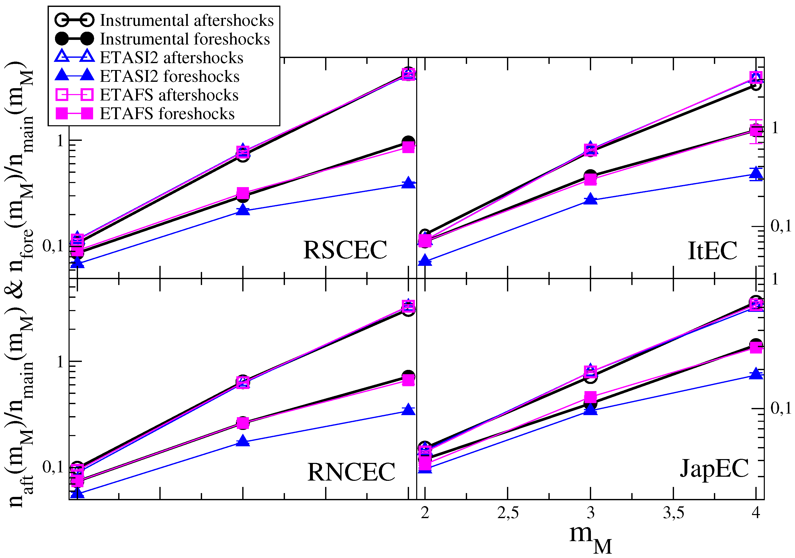
In Figure 1, we plot the ratio between aftershock and mainshock number for different mainshock classes and for the different instrumental catalogs. We also plot the ratio between foreshock and mainshock number .
Results in Figure 1 show that the aftershock number is systematically larger than the foreshock number and this difference increases for increasing . The aftershock number is consistent with the Utsu-productivity law (A1)
and a similar law is also observed for foreshocks .
3.3. Aftershock and Foreshock Spatial Distribution
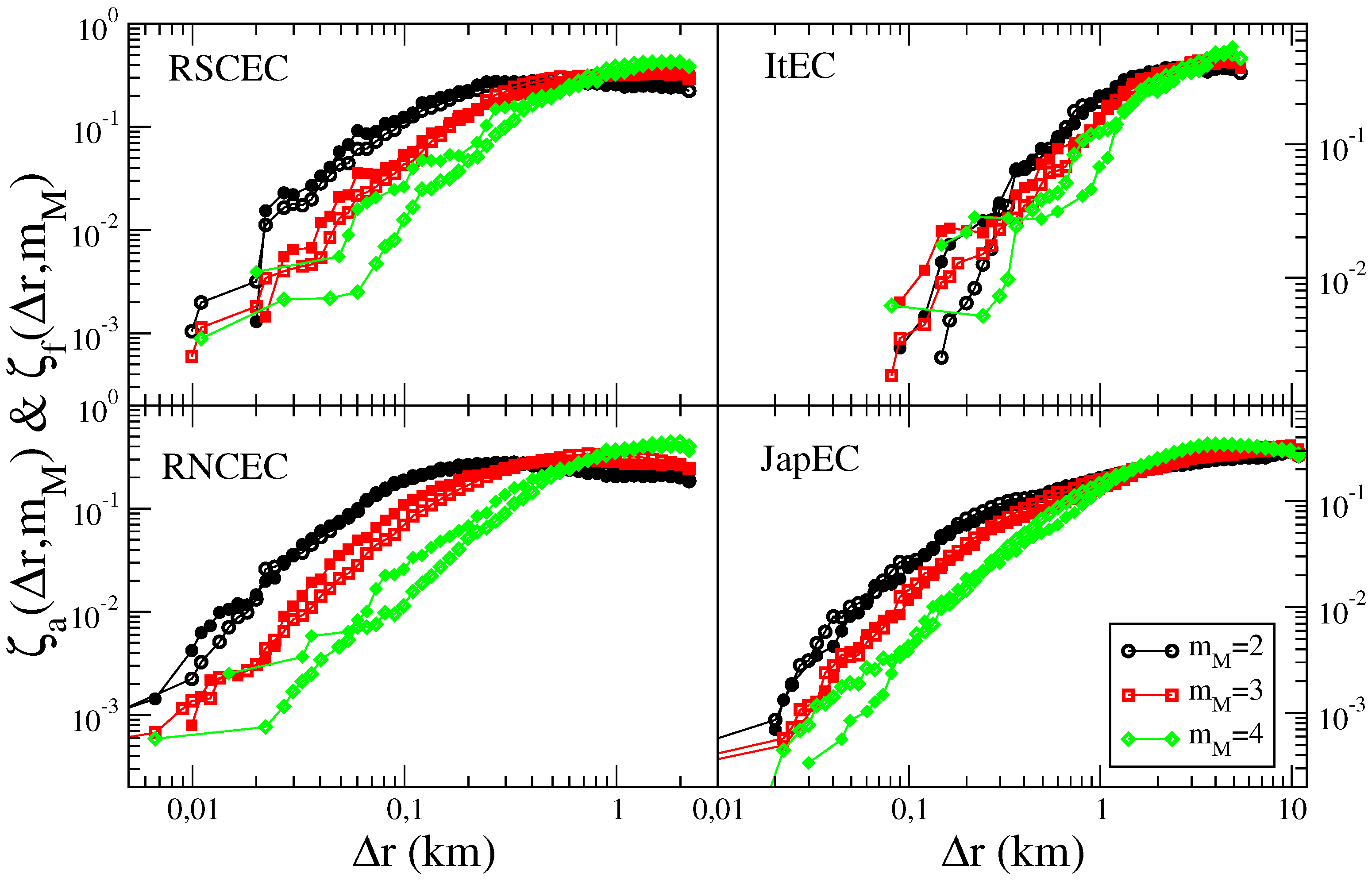
In Figure 2 we plot, for different catalogs, the average epicentral distance defined as as , were is the aftershock epicentral distribution. We also define the average foreshock epicentral distance
where is the foreshock epicentral distribution.
4. Results in Numerical Catalogs
4.1. Results in the ETAS Catalog
The Aftershock and Foreshock Number in the ETAS Catalog
In Figure 1, we compare results for and with the results obtained applying the same definition of aftershocks, mainshocks and foreshocks to ETAS catalogs. The values of both and depend on the parameters (Equation (2)) of the numerical model. In particular, in first approximation, neglecting the contribution of background events from Equation (2) we obtain
which indicates that the ETAS model can reproduce the experimental result Equation (6) with .
In numerical simulations we have explored a wide range of ETAS parameters and verified that there exists a set of parameters leading to ETAS catalogs with the same behavior of of the instrumental ones. In all cases the agreement between ETAS and instrumental catalogs is always recovered for values of . We wish to stress the difference between and : is the model parameter which controls the productivity law in numerical simulations whereas is the value obtained applying our definition of mainshock and aftershock to ETAS catalogs and then performing a fit according to Equation (6). The small discrepancies between and can be attributed to the background contribution which weakly affects data at small whereas it can be neglected for increasing .
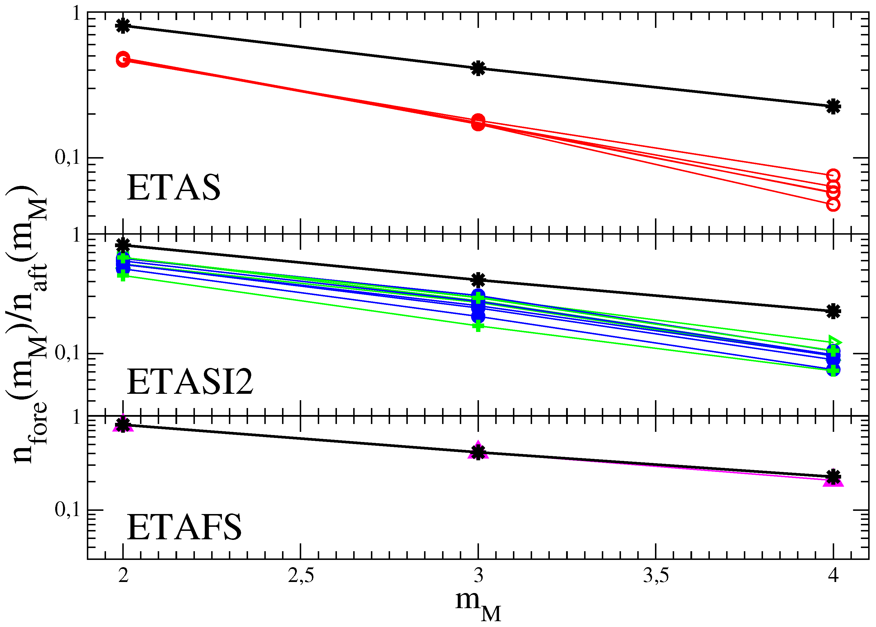
A central observation is that all choices of parameters producing agreement in between ETAS and instrumental catalogs give a value of in ETAS catalogs systematically smaller than the instrumental value. It is difficult to obtain a simple approximated expression for the foreshock number as function of as in Equation (7). However, it is reasonable to expect that the ratio is mainly controlled by the parameter and weakly depends on the other model parameters. This is supported by numerical simulations where we fix in order to have the same value of in ETAS catalogs. Results plotted in Figure 3 show that different choices of lead to similar results for , in all cases, significantly smaller than the experimental value for any .
4.2. Aftershock and Foreshock Spatial Distribution in the ETAS Catalog
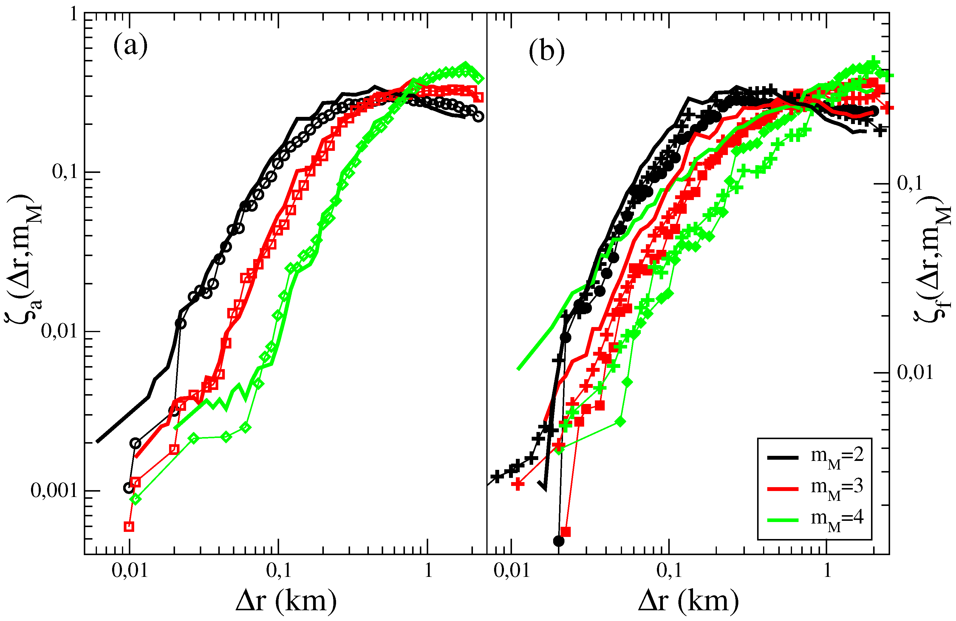
The average spatial distribution of aftershocks and foreshocks in ETAS catalogs is plotted in Figure 4. Results show that even if one can generate ETAS catalogs with in good agreement with instrumental catalogs (Figure 4a), significant differences are observed between the numeric and the experimental (Figure 4b). This difference becomes more pronounced for increasing and can simply attributed to the nature of foreshocks in the ETAS model which are typical events that have triggered a larger shock. Indeed, neglecting the contribution of background seismicity, we indicate by the probability that an event with magnitude triggers an earthquake with magnitude m inside a temporal window T. The epicentral distribution is approximatively given by . To evaluate the aftershock epicentral distribution we must restrict to triggered events with and integrate over all values of ,
Conversely, to evaluate we must consider triggered earthquakes with and since m is identified as a mainshock, its magnitude is constrained in the interval . Taking into account that the magnitude of the triggering earthquake , identified as a foreshock, is inside the interval we obtain
We wish to stress the fundamental difference between Equations (8) and (9) due to the inversion between m and of the integration range. In Equation (8) the spatial distance is controlled by the kernel which depends on and if . Conversely, in Equation (9) and if , since is an exponential decreasing function of m, the integral in Equation (9) is mainly controlled by the contribution from which leads to . As a consequence, in the ETAS model, we expect that only weakly depends on differently from . The comparison between Equations (8) and (9) therefore shows that independently of the value of the model parameters, the condition cannot be reproduced by the ETAS model. This is confirmed by Figure 4 where the symmetrical behavior , observed in the instrumental catalogs, is not recovered in the ETAS catalogs. Equations (8) and (9) also indicate that is substantially independent of the value of whereas is expected to significantly depend on it, in agreement with numerical simulations of the ETAS model [29]. In instrumental catalogs, conversely, the symmetry is observed quite independently of the value of [29]. This is another important difference of the spatial distribution of foreshocks between instrumental and ETAS catalogs.
4.3. Results in the ETASI2 Catalog
Results of the previous section show that ETAS catalogs contain fewer aftershocks than instrumental catalogs. A possible explanation of the foreshock deficit is related to the difficulty to identify small events which occur soon after larger ones as discussed in Section 2.2. This makes instrumental catalog incomplete in the first part of the aftershock sequence. As a consequence, the value of A, implemented in the ETAS model to recover the instrumental ratio , is underestimated as well as the ratio of . In this section we take explicitly into account the role of incompleteness by studying aftershocks and foreshocks statistical feature in the ETASI2 catalog.
We have performed extended numerical simulations of the ETASI2 model exploring a wide range of model parameters and evaluated and . Restricting to parameters with in agreement with the instrumental RSCEC catalog, we find (Figure 3) that, as expected, the incompleteness increases the value of which, however, still remains systematically smaller than the value found in instrumental catalogs. For fixed and in Equation (3), the ratio does not strongly depend on different choices of , as well as on different values of and it is always significant smaller than the instrumental one. We also find that slightly increases for decreasing and becomes approximately independent for . However, also in this case the value is significantly smaller than the one measured in the instrumental catalogs. The origin of this discrepancy is that incompleteness also affects the foreshock number. Indeed, considering a mainshock of magnitude anticipated by an event (a foreshock) with magnitude , incompleteness does not only affect the identification of both and but it can hide foreshocks with magnitude occurring between them. Therefore, if the parameters are tuned in order to produce a higher aftershock incompleteness this also reduces the foreshock number and the experimental result is never recovered. In Figure 1 we plot for each instrumental catalog the results of the ETASI2 model for parameters leading to the best agreement for and minimizing the discrepancy for . Results are obtained assuming and for all catalogs, and keeping . Furthermore we use and s. The values of A and producing the best agreement are listed in the caption of Figure 1.
In numerical simulations (not shown) of the ETASI model we find that the spatial distribution of aftershocks in the ETASI2 and in the ETAS model are practically indistinguishable. Indeed, incompleteness typically affects the number of aftershocks but not their spatial distributions. The same observation also holds for the spatial distribution of foreshocks. Therefore, as in the ETAS model, the same deviations from the instrumental finding is also observed in ETASI2 catalogs.
4.4. Results in ETAFS Catalogs
Previous section have shown a systematic deficit of foreshocks in ETAS catalogs which cannot be attributed to the incompleteness of the instrumental catalogs. This motivates the addition of events, different from the ones already implemented in the ETAS catalogs, as in the ETAFS model (Section 2.3). In numerical simulations of the ETAFS model we fix s and chose the parameters , for each instrumental catalog, in order to reproduce the value , for different (see Table 1). We also take explicitly into account aftershock incompleteness, implemented as in the ETASI2 model, and finally generate synthetic catalogs with the same value of and as instrumental ones. Figure 3 shows that for all values of ETAFS catalogs contains the same number of both aftershocks and foreshocks of instrumental data sets.
Interestingly, adding the “extra” foreshocks allows us to generate numerical catalogs which reproduce also the result , observed in instrumental catalogs (Figure 2). Indeed, in (Figure 4) we compare the average fore-mainshock distance between the ETAFS and the RSCEC catalog and obtain satisfactory agreement for all values of .
5. Conclusions
We have shown that in four different instrumental regional catalogs, the configuration where a smaller earthquake precedes the occurrence of a larger one occurs more frequently than what expected according to the ETAS model. Furthermore, the average spatial distance between the two earthquakes in instrumental catalogs is significantly larger than predicted by the ETAS model. These results support the idea that the preparatory phase of an earthquake can be accompanied by the nucleation of small earthquakes, a mechanism expected according to the nucleation theory [13,14,15] but not present in the ETAS model. We have therefore presented a novel model which, together with the usual aftershock triggering, assumes that an earthquake can be anticipated by the occurrence of smaller ones. The occurrence probability of these small events is formalized on the basis of statistical empirical features of foreshocks without any a priori physical explanation. The model is supported by its efficiency in reproducing statistical features of both aftershocks and foreshocks in instrumental catalogs.
All properties investigated in this study are obtained by means of a stacking procedure. An interesting point is the behavior expected according to the ETAFS model for the seismic activity before a single large shock. The best-fit parameters of the ETAFS model (Table 1) indicate a small coefficient in the foreshock productivity law and accordingly the number of foreshock remains relatively small also before large . For instance, we expect on average less than 8 () foreshocks the day before a magnitude mainshock, within a radius of 10 km. This small number implies that for a single mainshock, foreshock activity can at most appear in the form of isolated bursts not leading to an evident systematic increase of the seismic rate. This is consistent with experimental observations, where the inverse Omori-law is obtained only after a stacking procedure and rarely observed inside isolated sequences [59,60].
The agreement with experimental data suggests that the ETAFS model can contribute to a significant improvement of pre-seismic forecasting. A rigorous validation of this point, however, needs to be tested in prospective tests. Unfortunately, a main limitation of the model is that it is not immediately suitable to be implemented in this kind of analysis. Indeed, in order to forecast the occurrence of an earthquake, according to the ETAFS model it is necessary to distinguish foreshock from normal earthquake triggering. An attempt in this direction can be found in [17] where the ETAS occurrence probability is multiplied by an ad-hoc function which gives different weights to aftershock and foreshock clustering. This produces significant gain in the retrospective forecasting of earthquakes. The nature of foreshocks implemented in the ETAFS model is consistent with this approach promoting further studies on the relevance of foreshocks in seismic forecasting.
Author Contributions
All authors contributed equally to the conceptualization, the formal analysis and the writing of this manuscript.
Funding
This research received no external funding.
Acknowledgments
We thank the National Research Institute for Earth Science and Disaster Prevention for the mainland Japan catalog.
Conflicts of Interest
The authors declare no conflict of interest.
References
- Ogata, Y. Statistical Models for Earthquake Occurrences and Residual Analysis for Point Processes. J. Am. Stat. Assoc. 1988, 83, 9–27. [Google Scholar] [CrossRef]
- Ogata, Y. Space-time Point-process Models for Earthquake Occurrences. Ann. Inst. Stat. Math. 1988, 50, 379–402. [Google Scholar] [CrossRef]
- Ogata, Y. A Monte Carlo method for high dimensional integration. Numer. Math. 1989, 55, 137–157. [Google Scholar] [CrossRef]
- Huang, Q.; Gerstenberger, M.; Zhuang, J. Current Challenges in Statistical Seismology. Pure Appl. Geophys. 2016, 173, 1–3. [Google Scholar] [CrossRef] [Green Version]
- Corral, A. Long-Term Clustering, Scaling, and Universality in the Temporal Occurrence of Earthquakes. Phys. Rev. Lett. 2004, 92, 108501. [Google Scholar] [CrossRef] [PubMed]
- Corral, A. Renormalization-Group Transformations and Correlations of Seismicity. Phys. Rev. Lett. 2005, 95, 028501. [Google Scholar] [CrossRef] [PubMed]
- Corral, A. Scaling and universality in the dynamics of seismic occurrence and beyond. In Acoustic Emission and Critical Phenomena; CRC Press: Boca Raton, FL, USA, 2008; pp. 225–244. [Google Scholar]
- Bottiglieri, M.; de Arcangelis, L.; Godano, C.; Lippiello, E. Multiple-Time Scaling and Universal Behavior of the Earthquake Interevent Time Distribution. Phys. Rev. Lett. 2010, 104, 158501. [Google Scholar] [CrossRef] [PubMed]
- Lippiello, E.; Corral, A.; Bottiglieri, M.; Godano, C.; de Arcangelis, L. Scaling behavior of the earthquake intertime distribution: Influence of large shocks and time scales in the Omori law. Phys. Rev. E 2012, 86, 066119. [Google Scholar] [CrossRef] [PubMed]
- Varotsos, P.A.; Sarlis, N.V.; Skordas, E.S.; Tanaka, H.K.; Lazaridou, M.S. Attempt to distinguish long-range temporal correlations from the statistics of the increments by natural time analysis. Phys. Rev. E 2006, 74, 021123. [Google Scholar] [CrossRef]
- Sarlis, N.V.; Skordas, E.S.; Varotsos, P.A. Nonextensivity and natural time: The case of seismicity. Phys. Rev. E 2010, 82, 021110. [Google Scholar] [CrossRef]
- de Arcangelis, L.; Godano, C.; Grasso, J.R.; Lippiello, E. Statistical physics approach to earthquake occurrence and forecasting. Phys. Rep. 2016, 628, 1–91. [Google Scholar] [CrossRef]
- Ohnaka, M. Earthquake source nucleation: A physical model for short-term precursors. Tectonophysics 1992, 211, 149–178. [Google Scholar] [CrossRef]
- Ohnaka, M. Critical Size of the Nucleation Zone of Earthquake Rupture Inferred from Immediate Foreshock Activity. J. Phys. Earth 1993, 41, 45–56. [Google Scholar] [CrossRef]
- Dodge, D.A.; Beroza, G.C.; Ellsworth, W.L. Detailed observations of California foreshock sequences: Implications for the earthquake initiation process. J. Geophys. Res. Solid Earth 1996, 101, 22371–22392. [Google Scholar] [CrossRef] [Green Version]
- Brodsky, E.E. The spatial density of foreshocks. Geophys. Res. Lett. 2011, 38, L10305. [Google Scholar] [CrossRef]
- Lippiello, E.; Marzocchi, W.; de Arcangelis, L.; Godano, C. Spatial organization of foreshocks as a tool to forecast large earthquakes. Sci. Rep. 2012, 2, 846. [Google Scholar] [CrossRef] [PubMed]
- Shearer, P.M. Self-similar earthquake triggering, Bath’s law, and foreshock/aftershock magnitudes: Simulations, theory, and results for Southern California. J. Geophys. Res.-Solid Earth 2012, 117. [Google Scholar] [CrossRef]
- Shearer, P.M. Space-time clustering of seismicity in California and the distance dependence of earthquake triggering. J. Geophys. Res. Solid Earth 2012, 117. [Google Scholar] [CrossRef] [Green Version]
- Hainzl, S. Comment on “Self-similar earthquake triggering, Båth’s law, and foreshock/aftershock magnitudes: Simulations, theory, and results for southern California” by P. M. Shearer. J. Geophys. Res. Solid Earth 2013, 118, 1188–1191. [Google Scholar] [CrossRef]
- Shearer, P.M. Reply to comment by S. Hainzl on “Self-similar earthquake triggering, Båth’s Law, and foreshock/aftershock magnitudes: Simulations, theory and results for southern California”. J. Geophys. Res. Solid Earth 2013, 118, 1192. [Google Scholar] [CrossRef]
- Bouchon, M.; Durand, V.; Marsan, D.; Karabulut, H.; Schmittbuhl, J. The long precursory phase of most large interplate earthquakes. Nat. Geosci. 2013, 6, 299–302. [Google Scholar] [CrossRef]
- Mignan, A. The debate on the prognostic value of earthquake foreshocks: A meta-analysis. Sci. Rep. 2014, 4, 4099–4103. [Google Scholar] [CrossRef] [PubMed]
- Chen, X.W.; Shearer, P.M. California foreshock sequences suggest aseismic triggering process. Geophys. Res. Lett. 2013, 40, 2602–2607. [Google Scholar] [CrossRef] [Green Version]
- Brodsky, E.E.; Lay, T. Recognizing Foreshocks from the 1 April 2014 Chile Earthquake. Science 2014, 344, 700–702. [Google Scholar] [CrossRef] [Green Version]
- Ogata, Y.; Katsura, K. Comparing foreshock characteristics and foreshock forecasting in observed and simulated earthquake catalogs. J. Geophys. Res. Solid Earth 2014, 119, 8457–8477. [Google Scholar] [CrossRef] [Green Version]
- Felzer, K.R.; Page, M.T.; Michael, A.J. Artificial seismic acceleration. Nat. Geosci. 2015, 8, 82–83. [Google Scholar] [CrossRef]
- Bouchon, M.; Marsan, D. Reply to ‘Artificial seismic acceleration’. Nat. Geosci. 2015, 8, 83. [Google Scholar] [CrossRef]
- Lippiello, E.; Giacco, F.; Marzocchi, W.; Godano, C.; Arcangelis, L.D. Statistical Features of Foreshocks in Instrumental and ETAS Catalogs. Pure Appl. Geophys. 2017, 1–19. [Google Scholar] [CrossRef]
- Seif, S.; Zechar, J.D.; Mignan, A.; Nandan, S.; Wiemer, S. Foreshocks and Their Potential Deviation from General SeismicityForeshocks and Their Potential Deviation from General Seismicity. Bull. Seismol. Soc. Am. 2018, 109. [Google Scholar] [CrossRef]
- Kagan, Y.Y. Short-Term Properties of Earthquake Catalogs and Models of Earthquake Source. Bull. Seismol. Soc. Am. 2004, 94, 1207–1228. [Google Scholar] [CrossRef]
- Helmstetter, A.; Kagan, Y.Y.; Jackson, D.D. Comparison of Short-Term and Time-Independent Earthquake Forecast Models for Southern California. Bull. Seismol. Soc. Am. 2006, 96, 90–106. [Google Scholar] [CrossRef] [Green Version]
- Enescu, B.; Mori, J.; Miyazawa, M. Quantifying early aftershock activity of the 2004 mid-Niigata Prefecture earthquake (Mw6.6). J. Geophys. Res. Solid Earth 2007, 112, B04310. [Google Scholar] [CrossRef]
- Peng, Z.; Vidale, J.E.; Ishii, M.; Helmstetter, A. Seismicity rate immediately before and after main shock rupture from high-frequency waveforms in Japan. J. Geophys. Res. Solid Earth 2007, 112, B03306. [Google Scholar] [CrossRef]
- Peng, Z.; Zhao, P. Migration of early aftershocks following the 2004 Parkfield earthquake. Nat. Geosci. 2009, 2, 877–881. [Google Scholar] [CrossRef]
- Omi, T.; Ogata, Y.; Hirata, Y.; Aihara, K. Forecasting large aftershocks within one day after the main shock. Sci. Rep. 2013, 3, 2218. [Google Scholar] [CrossRef] [PubMed]
- Lippiello, E.; Cirillo, A.; Godano, G.; Papadimitriou, E.; Karakostas, V. Real-time forecast of aftershocks from a single seismic station signal. Geophys. Res. Lett. 2016, 43, 6252–6258. [Google Scholar] [CrossRef]
- Hainzl, S. Apparent triggering function of aftershocks resulting from rate-dependent incompleteness of earthquake catalogs. J. Geophys. Res. Solid Earth 2016, 121, 6499–6509. [Google Scholar] [CrossRef] [Green Version]
- Hainzl, S. Rate-Dependent Incompleteness of Earthquake Catalogs. Seismol. Res. Lett. 2016, 87, 337–344. [Google Scholar] [CrossRef]
- de Arcangelis, L.; Godano, C.; Lippiello, E. The overlap of aftershock coda-waves and short-term post seismic forecasting. J. Geophys. Res. Solid Earth 2018, 123, 5661–5674. [Google Scholar] [CrossRef]
- Shcherbakov, R.; Yakovlev, G.; Turcotte, D.L.; Rundle, J.B. Model for the Distribution of Aftershock Interoccurrence Times. Phys. Rev. Lett. 2005, 95, 218501. [Google Scholar] [CrossRef]
- Lippiello, E.; Bottiglieri, M.; Godano, C.; de Arcangelis, L. Dynamical scaling and generalized Omori law. Geophys. Res. Lett. 2007, 34, L23301. [Google Scholar] [CrossRef]
- Bottiglieri, M.; de Arcangelis, L.; Godano, C.; Lippiello, E. The Generalized Omori law: Magnitude incompleteness or magnitude clustering. Int. J. Mod. Phys. B 2009, 23, 5597–5608. [Google Scholar] [CrossRef]
- Bottiglieri, M.; Lippiello, E.; Godano, C.; de Arcangelis, L. Identification and spatiotemporal organization of aftershocks. J. Geophys. Res. Solid Earth 2009, 114, B03303. [Google Scholar] [CrossRef]
- Bottiglieri, M.; Lippiello, E.; Godano, C.; de Arcangelis, L. Comparison of branching models for seismicity and likelihood maximization through simulated annealing. J. Geophys. Res. Solid Earth 2011, 116, B02303. [Google Scholar] [CrossRef]
- Davidsen, J.; Baiesi, M. Self-similar aftershock rates. Phys. Rev. E 2016, 94, 022314. [Google Scholar] [CrossRef] [PubMed]
- Lippiello, E.; Godano, C.; de Arcangelis, L. Dynamical Scaling in Branching Models for Seismicity. Phys. Rev. Lett. 2007, 98, 098501. [Google Scholar] [CrossRef] [PubMed]
- Lippiello, E.; de Arcangelis, L.; Godano, C. Influence of Time and Space Correlations on Earthquake Magnitude. Phys. Rev. Lett. 2008, 100, 038501. [Google Scholar] [CrossRef]
- Lippiello, E.; de Arcangelis, L.; Godano, C. Time, Space and Magnitude Correlations in Earthquake Occurrence. Int. J. Mod. Phys. B 2009, 23, 5583–5596. [Google Scholar] [CrossRef]
- Lippiello, E.; de Arcangelis, L.; Godano, C. Role of Static Stress Diffusion in the Spatiotemporal Organization of Aftershocks. Phys. Rev. Lett. 2009, 103, 038501. [Google Scholar] [CrossRef]
- Sarlis, N.V. Magnitude correlations in global seismicity. Phys. Rev. E 2011, 84, 022101. [Google Scholar] [CrossRef]
- Lippiello, E.; Godano, C.; de Arcangelis, L. The earthquake magnitude is influenced by previous seismicity. Geophys. Res. Lett. 2012, 39, L05309. [Google Scholar] [CrossRef]
- Lippiello, E.; Godano, C.; de Arcangelis, L. Magnitude correlations in the Olami-Feder-Christensen model. Europhys. Lett. 2013, 102, 59002. [Google Scholar] [CrossRef]
- Hauksson, E.; Shearer, P.; Yang, W. Waveform relocated earthquake catalog for Southern California (1981 to June 2011). Bull. Seismol. Soc. Am. 2012, 102, 2239–2244. [Google Scholar] [CrossRef]
- Waldhauser, F.; Schaff, D.P. Large-scale relocation of two decades of Northern California seismicity using cross-correlation and double-difference methods. J. Geophys. Res. Solid Earth 2008, 113, B08311. [Google Scholar] [CrossRef]
- I.S.I.D.E. Italian Seismological Instrumental and Parametric Data-Base. Available online: http://cnt.rm.ingv.it/en/iside (accessed on 11 February 2019).
- From Japan Meteorological Agency Earthquake Catalog, provided by N.I.E.D. Available online: https://wwweic.eri.u-tokyo.ac.jp/db/jma/index.html (accessed on 11 February 2019).
- Felzer, K.R.; Brodsky, E.E. Decay of aftershock density with distance indicates triggering by dynamic stress. Nature 2006, 441, 735–738. [Google Scholar] [CrossRef] [PubMed]
- Papadopoulos, G.A.; Charalampakis, M.; Fokaefs, A.; Minadakis, G. Strong foreshock signal preceding the L’Aquila (Italy) earthquake (Mw 6.3) of 6 April 2009. Nat. Hazards Earth Syst. Sci. 2010, 10, 19–24. [Google Scholar] [CrossRef]
- Daskalaki, E.; Spiliotis, K.; Siettos, C.; Minadakis, G.; Papadopoulos, G.A. Foreshocks and Short-Term Hazard Assessment to Large Earthquakes using Complex Networks: the Case of the 2009 L’Aquila Earthquake. Nonlinear Process. Geophys. Discuss. 2016, 2016, 1–20. [Google Scholar] [CrossRef]
Figure 1.
(Color online) The ratio and in instrumental and synthetic catalogs. Different panels correspond to different instrumental catalogs. We use open symbols for and filled symbols for . Results from the instrumental data sets are indicated with black circles. Green triangles are results for the ETASI2 model and red squares for the ETAFS model. The error bars (of the same size of symbols) in numerical catalogs represent the standard deviation from 100 realization of synthetic catalogs. The best parameter of the ETAFS model are listed in Table 1 whereas for the ETASI2 model the best agreement is obtained with , and for RSCEC, , and for RNCEC, , and for ItEC and , and for JapEC.

Figure 2.
(Color online) The average distance of aftershocks (open symbols) and of foreshocks (filled symbols) is plotted as function of for the different catalogs. Different mainshock magnitude classes are plotted with different colors and symbols.
Figure 2.
(Color online) The average distance of aftershocks (open symbols) and of foreshocks (filled symbols) is plotted as function of for the different catalogs. Different mainshock magnitude classes are plotted with different colors and symbols.

Figure 3.
(Color online) The ratio in the RSCEC catalog (black stars) is compared with the value obtained in synthetic ETAS (upper panel), ETASI2 (central panel) and ETAFS (lower panel) catalog. (Upper panel) The red open symbols are results for the ETAS model for different choices of the parameters , and . (Central Panel) The blue filled symbols are results for the ETASI2 model implementing Equation (3) with and and for different choices of the parameters , and . Green symbols correspond to , and used in Figure 1 for the RSCEC catalog and considering different values of , and . (Lower panel) The filled magenta up triangles are results of the ETAFS model with the best set of parameters listed in Table 1.

Figure 4.
(Color online) (Left panel) The average distance of aftershocks in the RSCEC (open symbols) and in the synthetic ETASI2 catalogs (continuous lines) is plotted as function of for different mainshock magnitude classes. (Right Panel) The average distance of foreshocks in the RSCEC (filled symbols) and in the synthetic ETASI2 catalog (continuous lines) is plotted as function of for different mainshock magnitude classes. Results for the EATFS model, for the best set of model parameters listed in Table 1, are plotted with crosses.


Table 1.
Best parameters of the ETAFS model.
| Catalog | A | B | s−1 | ||
|---|---|---|---|---|---|
| RSCEC | 0.084 | 0.9 | 0.050 | 0.54 | 5.84 × 10⁻⁴ |
| RNCEC | 0.082 | 0.88 | 0.033 | 0.59 | 4.98 × 10⁻⁴ |
| ItEC | 0.086 | 0.88 | 0.052 | 0.60 | 5.21 × 10⁻⁴ |
| JapEC | 0.234 | 0.6 | 0.160 | 0.36 | 5.92 × 10⁻³ |
© 2019 by the authors. Licensee MDPI, Basel, Switzerland. This article is an open access article distributed under the terms and conditions of the Creative Commons Attribution (CC BY) license (http://creativecommons.org/licenses/by/4.0/).
Share and Cite
MDPI and ACS Style
Lippiello, E.; Godano, C.; de Arcangelis, L. The Relevance of Foreshocks in Earthquake Triggering: A Statistical Study. Entropy 2019, 21, 173. https://0-doi-org.brum.beds.ac.uk/10.3390/e21020173
AMA Style
Lippiello E, Godano C, de Arcangelis L. The Relevance of Foreshocks in Earthquake Triggering: A Statistical Study. Entropy. 2019; 21(2):173. https://0-doi-org.brum.beds.ac.uk/10.3390/e21020173
Chicago/Turabian StyleLippiello, Eugenio, Cataldo Godano, and Lucilla de Arcangelis. 2019. "The Relevance of Foreshocks in Earthquake Triggering: A Statistical Study" Entropy 21, no. 2: 173. https://0-doi-org.brum.beds.ac.uk/10.3390/e21020173
Note that from the first issue of 2016, this journal uses article numbers instead of page numbers. See further details here.